Nonlinear Autonomous Systems of Differential

Transcription

1 Chapter 4 Nonlinear Autonomous Systems of Differential Equations 4.0 The Phase Plane: Linear Systems Introduction Consider a system of the form x = A(x), (4.0.1) where A is independent of t. Such a system is called an autonomous system.

2 286 Chapter 4. Below we consider the case where n = 2, i.e., dx dt = F(x,y) = A (1,1) x + A (1,2) y dy dt = G(x,y) = A (2,1) x + A (2,2) y. Suppose F and G are continuous and have continuous partial derivatives in some region D in the xy-plane (called the phase plane for the system). Then by the existence and uniqueness theorem, given any t 0 R and any point (x 0,y 0 ) D, there is a unique solution x = ϕ(t), y = ψ(t), (4.0.2) defined on an interval containing t 0, that satisfies the initial conditions ϕ(t 0 ) = x 0, ψ(t 0 ) = y 0. Note that (4.0.2) describe a parameterized curve in the phase plane.

3 4.0. The Phase Plane: Linear Systems 287 Phase Plane gives a graphical view on the movement of differential equation s solution without actually solving the equations. Such a curve is called a trajectory of the system. A plot that shows a representative sample of trajectories is called a phase portrait of the system.

4 288 Chapter 4. Definition A solution, (ϕ(t), ψ(t)), of equation x = A(x), is called a critical point (equilibrium solution) if it satisfies: x dx = 0. equivalent to dt = dy dt = 0. Note that tangent vectors to a trajectory is given by ( ϕ (t),ψ (t) ) = ( F(ϕ(t),ψ(t)),G(ϕ(t),ψ(t)) ). We can visualize the tangent vectors by evaluating ( F(x,y),G(x,y) ) at a large number of points in D and plotting the resulting vectors. The collection of all such tangent vectors is called the direction field of the system. The phase portrait various with the nature of the eigenvalues of A.

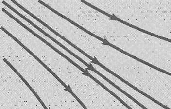
5 4.0. The Phase Plane: Linear Systems 289 Case I: Real Unequal Eigenvalues of the Same Sign The general solution of equation is: x = A(x), x = c 1 ξ (1) e r 1t + c 2 ξ (2) e r 2t where r 1 and r 2 are either both positive or both negative. Suppose first that r 1 < r 2 < 0, we re-write the above equation as: x = e r 2t [c 1 ξ (1) e (r 1 r 2 )t + c 2 ξ (2) ] Thus, as t, the trajectory not only approaches the origin, it also tends toward the line through ξ (2). All solutions approach the critical point tangent to ξ (2) except for those solutions that start exactly on the line through ξ (1).

6 290 Chapter 4. This type of critical point is called a node or a nodal sink. Figure 4.1: A node: r 1 < r 2 < 0. (a) The phase plane. (b) x 1 versus t

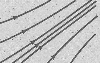
7 4.0. The Phase Plane: Linear Systems 291 Case II: Real Eigenvalues of Opposite Sign Again, the general solution of equation is: x = A(x), x = c 1 ξ (1) e r 1t + c 2 ξ (2) e r 2t WLOG, assume r 2 < 0 < r 1. (4.0.3) Suppose that the eigenvectors ξ (1) and ξ (2) are shown below. Figure 4.2: A saddle point: r 1 > 0, r 2 < 0. (a) The phase plane. (b) x 1 versus t. If the solution starts at an initial point on the line through ξ (1) (ξ (2) ), then x ( 0) as t. As positive exponential is the dominant term in

8 292 Chapter 4. equation (4.0.3), eventually all these solutions approach infinity asymptotic to the line determined by the eigenvector ξ (1) corresponding to the positive eigenvalue. The only solutions that approach the critical point at the origin are those that start precisely on the line determined by ξ (2). The origin is called a saddle point in this case.

9 4.0. The Phase Plane: Linear Systems 293 Case III: Equal Eigenvalues Consider eigenvalue is negative. (a) Two independent eigenvectors The general solution of equation is: x = A(x), x = c 1 ξ (1) e rt + c 2 ξ (2) e rt (4.0.4) Obviously, the ratio x 2 /x 1 is independent of t, but depends on the components of ξ (1) and ξ (2). The critical point is called a proper node (star point).

10 294 Chapter 4. Figure 4.3: A proper node, two independent eigenvectors: r 1 = r 2 < 0. (a) The phase plane. (b) x 1 versus t. (b) One independent eigenvector is: The general solution of equation x = A(x), x = c 1 ξe rt + c 2 (ξte rt + ηe rt ), (4.0.5) where ξ is the eigenvector and η is the generalized eigenvector. For large either positive or negative value of t, c 2 ξte rt is dominant, even if c 2 =0, the solution x = c 1 ξe rt lies on the line. Thus, each trajectory is asymptotic to a line

11 4.0. The Phase Plane: Linear Systems 295 parallel to ξ. The vector (c 1 ξ + c 2 η) + c 2 ξt determines the direction of x.

12 296 Chapter 4. Sketch 1. Draw the line (c 1 ξ +c 2 η)+c 2 ξt and note the direction of increasing t on this line. 2. The trajectory passes through the point c 1 ξ+ c 2 η when t = As t increase, the direction increase follows the directions of increasing t on the line, but the magnitude of x rapidly decreases and approach to zero. 4. As t decrease toward, the magnitude of x approaches infinity. Notice If r > 0, the trajectories are traversed in the outward direction. In this case, the critical point is called an improper or degenerate node.

13 4.0. The Phase Plane: Linear Systems 297 Figure 4.4: An improper node, one independent eigenvector; r 1 = r 2 < 0. (a) The phase plane. (b) x 1 versus t. (c) The phase plane. Case IV: Complex Eigenvalues Suppose that the eigenvalues are λ ± iµ, where both λ and µ are real, λ 0 and µ > 0. By simple calculation, we notice that ( ) λ µ A = µ λ

14 298 Chapter 4. The system is typified by: ( ) x λ µ = x (4.0.6) µ λ We introduce the polar coordinates r,θ given by r 2 = x x2 2, tan θ = x 2/x 1 (4.0.7) By differentiating these equations we obtain rr = x 1 x 1 +x 2x 2, (sec2 θ)θ = (x 1 x 2 x 2x 1 )/x2 1. (4.0.8) Substituting from equation (4.0.6) in the equation (4.0.8), we find that where c is a constant. r = λr r = ce λt

15 4.0. The Phase Plane: Linear Systems 299 Similarly, substituting from equation ( ) x λ µ = x µ λ in the equation θ = (x 1 x 2 x 2x 1 )/x2 1 and using the fact that sec 2 θ = tan 2 θ+1 = r2, and hence θ = µ θ = µt + θ 0 (4.0.9) As µ > 0, θ decreases as t increases, and the direction of motion on a trajectory is clockwise. As t, r 0 if λ < 0 and r if λ > 0. The trajectories are spirals, which approach from the origin depending on the sign of λ. The critical point is called a spiral point. x 2 1

16 300 Chapter 4. Notice: The trajectories are always spirals if λ 0. They are directed inward or outward respectively, depending on whether λ is negative or positive. Figure 4.5: A spiral point; r 1 = λ + iµ, r 2 = λ iµ. (a) λ < 0, the phase plane. (b) λ < 0, x 1 versus t. (c) λ > 0, the phase plane. (d) λ > 0, x 1 versus t.

17 4.0. The Phase Plane: Linear Systems 301 Example Consider dx dt dy = dt Figure 4.6: A spiral point; r = λ ± iµ with λ < 0. ( a b c d ) ( x y Look at the point (0,1) on the positive y-axis. dx dy = b, = d, if both b and d are negative, dt dt the trajectories move down and into the second quadrant. If λ < 0, the trajectories must be inward-pointing spirals. )

18 302 Chapter 4. Case V: Pure Imaginary Eigenvalues In this case λ = 0 and the system become: ( ) x 0 µ = x (4.0.10) µ 0 with eigenvalues ±iµ. It is easy to proof that r = c, θ = µt + θ 0. where both c and θ 0 are constants. Thus, the trajectories are circles with center at the origin, that are traversed clockwise (anticlockwise) if µ > 0 (µ < 0). A complete circuit about the origin is made in a time interval of length 2π/µ, so all solutions are periodic with period 2π/µ. The critical point is called a center. In general, when the eigenvalues are pure imaginary, it is possible to show that the trajectories are ellipses centered at the origin.

19 4.0. The Phase Plane: Linear Systems 303 A typical situation is shown in Figure 4.7, which also shows some typical graphs of x 1 versus t. Figure 4.7: A center; r 1 = iµ, r 2 = iµ. (a) The phase plane. (b) x 1 versus t. According to these five cases, we can make several observations: 1 When t, each trajectory either approaches infinity, approaches the critical point x = 0, or repeatedly traverses a closed curve, corresponding to a periodic solution, that surrounds the critical point.

20 304 Chapter 4. 2 Through each point (x 0,y 0 ) in the phase plane there is only one trajectory; thus the trajectories do not cross each other. Do not be misled by the figures, in which it sometimes appears that many trajectories (actually, only one) pass through the critical point x = 0. The other solutions that appear to pass through the origin actually only approach this point as t or.

21 4.0. The Phase Plane: Linear Systems The set of all trajectories is either: (a) All trajectories approach the critical point x = 0 as t. This is the case if the eigenvalues are negative (real part). The origin is either a nodal or a spiral sink. (b) All trajectories remain bounded but do not approach the origin as t. This is the case if the eigenvalues are pure imaginary. (The origin is a center) (c) Some trajectories, and possibly all trajectories except x = 0, tend to infinity as t. This is the case if at least one of the eigenvalues is positive (real part). The origin is either a nodal source, a spiral source, or a saddle point.

22 306 Chapter 4. Stability and Instability. x = f(x) (4.0.11) In the following definitions, we use the notation x to designate the length, or magnitude, of the vector x. The points, if any, where f(x) = 0 are called critical points of the autonomous system. x 0 is said to be stable if, given any ǫ > 0, there is a δ > 0 such that every solution x = φ(t) of the system, which at t = 0 satisfies φ(0) x 0 < δ (4.0.12) exists for all positive t and satisfies for all t 0. φ(t) x 0 < ǫ (4.0.13)

23 4.0. The Phase Plane: Linear Systems 307 This is illustrated geometrically in Figures 4.8a and 4.8b. Figure 4.8: (a) Asymptotic stability. (b) Stability If all solutions that start sufficiently close to x 0, then it stays close to x 0. Note that in Figure 4.8a the trajectory is within the circle x x 0 = δ at t = 0 and, while it soon passes outside of this circle, it remains within the circle x x 0 = ǫ for all t 0. However, the trajectory of the solution does not have to approach the critical point x 0 as t, as illustrated in Figure 4.8b.

24 308 Chapter 4. A critical point that is not stable is said to be unstable. A critical point x 0 is said to be asymptotically stable if it is stable and if there exists a δ 0, with 0 < δ 0 < δ, such that if a solution x = φ(t) satisfies φ(0) x 0 < δ 0, (4.0.14) then lim φ(t) = t x0. (4.0.15) Thus trajectories that start sufficiently close to x 0 must not only stay close but must eventually approach x 0 as t. This is the case for the trajectory in Figure 4.8a but not for the one in Figure 4.8b. Note that asymptotic stability is a stronger property than stability. (4.0.15) is an essential feature of asymptotic stability, does not by itself imply even ordinary stability.

25 4.0. The Phase Plane: Linear Systems 309 Indeed, examples can be constructed in which all of the trajectories approach x 0 as t, but for which x 0 is not a stable critical point. Geometrically, all that is needed is a family of trajectories having members that start arbitrarily close to x 0, then depart an arbitrarily large distance before eventually approaching x 0 as t.

26 310 Chapter 4. In the undamped case, if the mass is displaced slightly from its lower equilibrium position, it will oscillate indefinitely with constant amplitude about the equilibrium position. This type of motion is stable, but not asymptotically stable. In general, undamped motion is impossible to achieve experimentally because the slightest degree of air resistance or friction at the point of support will eventually cause the pendulum to approach its rest position. Figure 4.9: Qualitative motion of a pendulum. (a) With air resistance. (b) With/without air resistance. (c) Without air resistance.

27 4.0. The Phase Plane: Linear Systems 311 Determination of Trajectories The trajectories of a two-dimensional autonomous system can sometimes be found by solving a related first order differential equation. From dx/dt = F(x,y), dy/dt = G(x,y), we have dy dx = dy/dt dx/dt = G(x,y) F(x,y). (4.0.16) which is a first order equation in the variables x and y. Observe that such a reduction is not usually possible if F and G depend also on t. If Equation (4.0.16) can be solved and if we write solutions (implicitly) in the form H(x, y) = c, (4.0.17) then Equation (4.0.17) is an equation for the trajectories of the system (4.0.16). In other words, the trajectories lie on the level curves of H(x,y).

28 312 Chapter 4. There is no general way of solving Equation (4.0.16) to obtain the function H, so this approach is applicable only in special cases.

29 4.0. The Phase Plane: Linear Systems 313 Example Find the trajectories of the system dx/dt = y, dy/dt = x. (4.0.18) In this case, Equation (4.0.16) becomes dy dx = x y. (4.0.19) This equation is separable since it can be written as ydy = xdx, and its solutions are given by H(x,y) = y 2 x 2 = c, (4.0.20) where c is arbitrary. Therefore the trajectories of the system (4.0.18) are the hyperbolas shown in Figure The direction of motion on the trajectories can be inferred from the fact that both dx/dt and dy/dt are positive in the first quadrant. The only critical point is the saddle point at the origin. Actually, the solution is: x = c 1 e t + c 2 e t, y = c 1 e t c 2 e t.

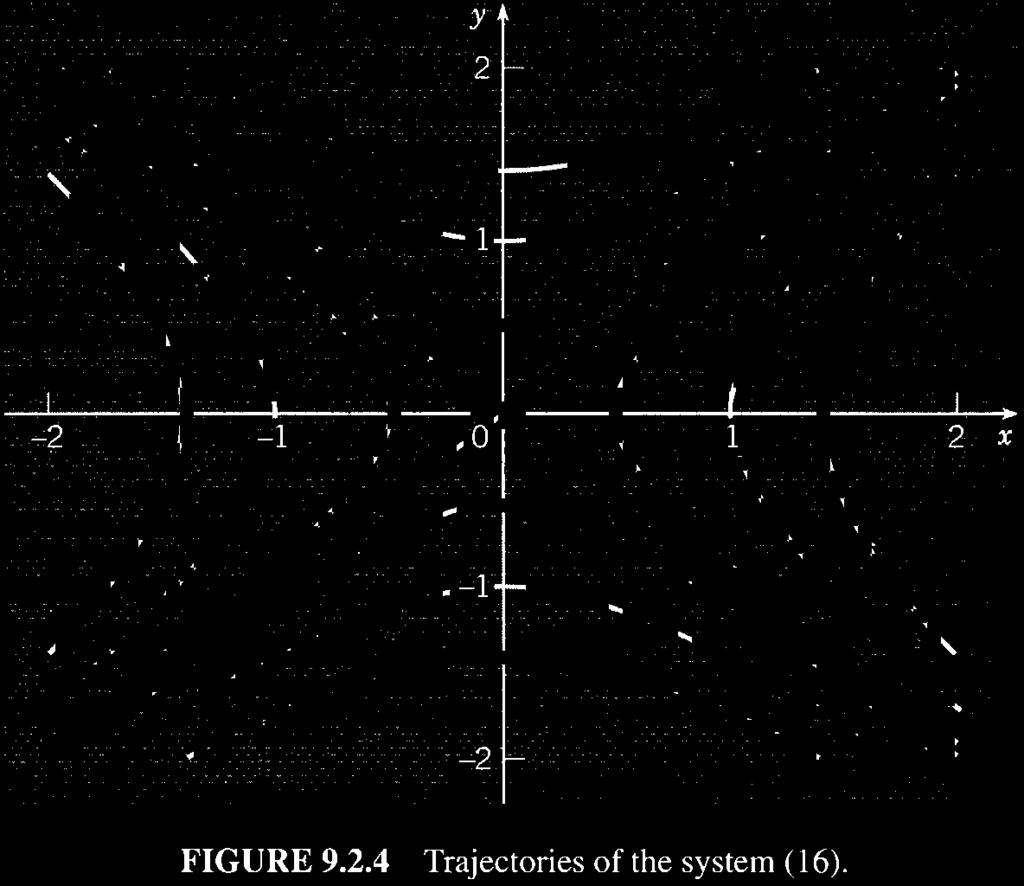
30 314 Chapter 4. Figure 4.10: Trajectories of the system.

31 4.0. The Phase Plane: Linear Systems 315 Example Find the trajectories of the system dx dt = 4 2y, dy dt = 12 3x2. (4.0.21) From the equations 4 2y = 0, 12 3x 2 = 0 The critical points are (-2, 2) and (2, 2). Based on the given system, we have dy dx = 12 3x2 4 2y. (4.0.22) Separating the variables and integrating, solutions satisfy H(x,y) = 4y y 2 12x + x 3 = c, (4.0.23) where c is an arbitrary constant. The direction of motion on the trajectories can be determined by drawing a direction field for the system (4.0.21), or by evaluating dx/dt and dy/dt at one or two selected points.

32 316 Chapter 4. Figure 4.11: Trajectories of the system. From Figure 4.11 you can see that the critical point (2, 2) is a saddle point while the point (-2, 2) is a center. Observe that one trajectory leaves the saddle point (at t = ), the methods of loops around the center, and returns to the saddle point (at t = + ).

33 4.1. Almost Linear Systems Almost Linear Systems x = Ax. (4.1.1) Recall that we required deta 0, so that x = 0 is the only critical point. Theorem The critical point x = 0 of the linear system dx/dt = F(x,y), dy/dt = G(x,y), is asymptotically stable if the eigenvalues r 1,r 2 are negative (real part); stable, but not asymptotically stable, if r 1 and r 2 are pure imaginary; unstable if r 1 and r 2 are real and either is positive (real part). Thus, the eigenvalues r 1, r 2 of A determine the type of critical point at x = 0 and its stability characteristics.

34 318 Chapter 4. When the system arises in some applied field, matrix A usually result from the measurements of certain physical quantities. Such measurements are often subject to small uncertainties, so it is of interest to investigate whether small changes in the coefficients can affect the stability or instability of a critical point and/or significantly alter the pattern of trajectories. Recall that the eigenvalues r 1, r 2 are the roots of the polynomial equation det(a ri) = 0. (4.1.2) It is possible to show that small perturbations in some or all the coefficients are reflected in small perturbations in the eigenvalues. The most sensitive situation occurs when r 1 = iµ, and r 2 = iµ, that is, when the critical point is a center and the trajectories are closed curves surrounding it.

35 4.1. Almost Linear Systems 319 If a slight change is made in the coefficients, then the eigenvalues r 1 and r 2 will take on new values r 1 = λ + iµ and r 2 = λ iµ, where λ is small in magnitude and µ = µ (see Figure 4.12). Figure 4.12: Schematic perturbation of r 1 = iµ, r 2 = iµ. If λ = 0, then the trajectories of the perturbed system become spirals. The system is asymptotically stable (unstable) if λ < 0 (> 0). Thus, small perturbations in the coefficients may well change the stability of the system and may alter radically the pattern of trajectories in the phase plane.

36 320 Chapter 4. If the eigenvalues r 1 = r 2, the critical point is a node. Small perturbations in the coefficients will cause r 1 r 2. If the separated roots are real, then the critical point of the perturbed system remains a node, but if the separated roots are complex conjugates, then the critical point becomes a spiral point. These two possibilities are shown schematically in Figure Figure 4.13: Schematic perturbation of r 1 = r 2 In this case the stability of the system is not affected by small perturbations in the coefficients, but the trajectories may be altered considerably.

37 4.1. Almost Linear Systems 321 In all other cases the stability of the system is not changed, nor is the type of critical point altered, by sufficiently small perturbations in the coefficients of the system. For example, if r 1 < r 2 < 0, then a small change in the coefficients will not change the sign of r 1 and r 2 nor allow them to be equal. The critical point remains an asymptotically stable node.

38 322 Chapter 4. For a nonlinear two-dimensional autonomous system x = f(x). (4.1.3) Our main object is to investigate the behavior of trajectories of the system (4.1.3) near a critical point x 0. Method: approximate the nonlinear system by an appropriate linear system. WLOG, we choose the critical point to be the origin as if x 0 0, we substitute u = x x 0. Then u will satisfy an autonomous system with a critical point at the origin.

39 4.1. Almost Linear Systems 323 Suppose that x = Ax + g(x), (4.1.4) and that x = 0 is an isolated critical point. I.e., there is some circle about the origin within which there are no other critical points. We assume that deta 0, so that x = 0 is also an isolated critical point of the linear system x = Ax.

40 324 Chapter 4. For the nonlinear system x = Ax + g(x), to be close to the linear system x = Ax we must assume that g(x) is small. Here, we assume that the components of g C 1 and g(x) / x 0 as x 0; (4.1.5) Such a system is called an almost linear system in the neighborhood of the critical point x = 0. Here, we let x T = (x,y) and r = x. Also, if g T (x) = (g 1 (x,y),g 2 (x,y)), then we have g 1 (x,y) g 0, 2 (x,y) 0 as r 0. r r (4.1.6)

41 4.1. Almost Linear Systems 325 Example Determine whether the system ( ) ( ) ( ) ( x 1 0 x x = + 2 xy y y 0.75xy 0.25y 2 (4.1.7) is almost linear in the neighborhood of the origin. ) Observe that (0, 0) is a critical point, and deta 0. The other critical points are (0, 2), (1, 0), and (0.5, 0.5); consequently, the origin is an isolated critical point. Here, we let x = r cosδ, y = r sin δ and g 1 (x,y) r as r 0. = x2 xy = r2 cos 2 δ r 2 sin δ cos δ r r = r(cos 2 δ + sin δ cos δ) 0 In a similar way, it can be shown that g 2 (x,y)/r 0 as r 0. Hence the system is almost linear near the origin.

42 326 Chapter 4. Example The motion of a pendulum is described by the system dx dt = y, dy dt = ω2 sinx γy. (4.1.8) The critical points are (0, 0), (±π, 0), (±2π, 0),..., so the origin is an isolated critical point of this system. Show that the system is almost linear near the origin. Solution To compare it with x = Ax + g(x), we must rewrite the given system so that the linear and nonlinear terms are clearly identified. If we write sin x = x + (sin x x) and substitute this expression in the second of Equation (4.1.8),

43 4.1. Almost Linear Systems 327 we obtain the equivalent system ( ) ( )( ( ) x 0 1 x = ) ω y ω γ y sinx x (4.1.9) On comparing it with x = Ax + g(x), we see that g 1 (x,y) = 0 and g 2 (x,y) = ω 2 (sin x x). From the Taylor series for sinx, we know that sin x x behaves like x 3 /3! = (r 3 cos 3 δ)/3! when x is small. Consequently, (sinx x)/r 0 as r 0. Thus the conditions (4.1.6) are satisfied and the system is almost linear near the origin.

44 328 Chapter 4. Let us now return to the general nonlinear system x = f(x), which we write in the scalar form x = F(x,y), y = G(x,y). (4.1.10) The system (4.1.10) is almost linear in the neighborhood of a critical point (x 0,y 0 ) whenever the functions F and G have continuous partial derivatives up to order two. To show this, use Taylor expansions about the point (x 0,y 0 ) to write F(x,y) and G(x,y) in the form F(x,y) = F(x 0,y 0 ) + F x (x 0,y 0 )(x x 0 ) +F y (x 0,y 0 )(y y 0 ) + η 1 (x,y), G(x,y) = G(x 0,y 0 ) + G x (x 0,y 0 )(x x 0 ) +G y (x 0,y 0 )(y y 0 ) + η 2 (x,y), where η 1 (x,y)/[(x x 0 ) 2 + (y y 0 ) 2 ] 1/2 0 as (x,y) (x 0,y 0 ), and similarly for η 2.

45 4.1. Almost Linear Systems 329 Note that F(x 0,y 0 ) = G(x 0,y 0 ) = 0, and that dx/dt = d(x x 0 )/dt and dy/dt = d(y y 0 )/dt. Then the system (4.1.10) reduces to d dt ( x x0 y y 0 ) = ( )( ) Fx (x 0, y 0 ) F y (x 0,y 0 ) x x0 G x (x 0, y 0 ) G y (x 0,y 0 ) y y ( ) 0 η1 (x,y) + (4.1.11) η 2 (x,y) or, in vector notation, du dt = df dx (x0 )u + η(x), (4.1.12) where u = (x x 0,y y 0 ) T and η = (η 1,η 2 ) T. (1) if the functions F and G are twice differentiable, then the system is almost linear and it is unnecessary to resort to the limiting process. (2) the linear system that approximates the nonlinear system near (x 0,y 0 ) is given by the linear part of Equations (4.1.11) or (4.1.12),

46 330 Chapter 4. d dt i.e., ( u1 u 2 ) = ( Fx (x 0,y 0 ) F y (x 0,y 0 ) G x (x 0,y 0 ) G y (x 0,y 0 ) where u 1 = x x 0 and u 2 = y y 0. )( u1 u 2 ), (4.1.13) Above equation provides a simple and general method for finding the linear system corresponding to an almost linear system near a given critical point.

47 4.1. Almost Linear Systems 331 Example Use ( ) ( )( ) d u1 Fx (x = 0,y 0 ) F y (x 0,y 0 ) u1, dt G x (x 0,y 0 ) G y (x 0,y 0 ) u 2 (where u 1 = x x 0 and u 2 = y y 0 ) to find the linear system corresponding to the pendulum equations dx dt = y, dy dt = ω2 sinx γy near the origin; near the critical point (π, 0). In this case F(x,y) = y, G(x,y) = ω 2 sin x γy; (4.1.14) since these functions are differentiable as many times as necessary, the former system is almost linear near each critical point. The derivatives of F and G are F x = 0, F y = 1, G x = ω 2 cosx, G y = γ. (4.1.15) u 2

48 332 Chapter 4. Thus, at the origin the corresponding linear system is ( ) ( )( ) d x 0 1 x = dt y ω 2. (4.1.16) γ y Similarly, evaluating the partial derivatives at (π, 0), we obtain ( ) ( ) ( ) d u 0 1 u = dt v ω 2, (4.1.17) γ v where u = x π, v = y. This is the linear system corresponding to dx dt = y, dy dt = ω2 sinx γy near the point (π, 0).

49 4.1. Almost Linear Systems 333 We now return to the almost linear system x = Ax + g(x). Since the nonlinear term g(x) is small compared to the linear term Ax when x is small, it is reasonable to hope that the trajectories of the linear system x = Ax, are good approximations to those of the nonlinear, at least near the origin.

50 334 Chapter 4. Linear System Almost Linear System r 1, r 2 Type Stability Type Stability r 1 > r 2 > 0 N Unstable N Unstable r 1 < r 2 < 0 N Asymptotically stable N Asymptotically stable r 2 < 0 < r 1 SP Unstable SP Unstable r 1 = r 2 > 0 PN or IN Unstable N or SpP Unstable r 1 = r 2 < 0 PN or IN Asymptotically stable N or SpP Asymptotically stable r 1, r 2 = λ ± iµ λ > 0 SpP Unstable SpP Unstable λ < 0 SpP Asymptotically stable SpP Asymptotically stable r 1 = µ, r 2 = µ C Stable C or SpP Indeterminate Note: N, node; IN, improper node; SP, saddle point; SpP, spiral point; C, center. Table 4.1: Stability Properties of Linear Systems x = Ax with det(a ri)=0 and det A 0 Theorem Let r 1 and r 2 be the eigenvalues of the linear system x = Ax, corresponding to the almost linear system x = Ax + g(x). Then the type and stability of the critical point (0, 0) of the linear system and the almost linear system are as shown in Table 4.1. Proof: Omit.

51 4.1. Almost Linear Systems 335 Remarks Theorem says that for small x (or x x 0 ) the nonlinear terms are also small and don t affect the stability and type of critical point as determined by the linear terms except in (1) r 1 and r 2 pure approximates imaginary, (2) r 1 and r 2 real and equal. Even if the critical point is of the same type, the trajectories may be different in appearance from those of the corresponding linear system, except very near the critical point. However, it can be shown that the slopes at which trajectories enter or leave the critical points are given correctly by the linear equation.

52 336 Chapter 4. Damped Pendulum. Near the origin dx dt = y, dy dt = ω2 sinx γy are approximated by the linear system ( ) ( d x 0 1 = dt y ω 2 γ whose eigenvalues are )( x y ), r 1,r 2 = γ ± γ 2 4ω 2. (4.1.18) 2 The nature of the solutions depend on the sign of γ 2 4ω 2 as follows. 1. If γ 2 4ω 2 > 0, then the eigenvalues are real, unequal and negative. The critical point (0, 0) is an asymptotically stable node of both systems. 2. If γ 2 4ω 2 = 0, then the eigenvalues are real, equal, and negative. The critical point (0, 0) is an asymptotically stable node of the linear system. It may be either an asymptotically stable node or spiral point of the almost linear system.

53 4.1. Almost Linear Systems If γ 2 4ω 2 < 0, then the eigenvalues are complex with negative real part. The critical point (0, 0) is an asymptotically stable spiral point of both systems. Thus the critical point (0, 0) is a spiral point of the system dx dt = y, dy dt = ω2 sinx γy if the damping is small and a node if the damping is large enough. In either case, the origin is asymptotically stable. In the case of γ 2 4ω 2 < 0, corresponding to small damping. The direction of motion on the spirals near (0, 0) can be obtained directly from dx dt = y, dy dt = ω2 sinx γy.

54 338 Chapter 4. Consider the point at which a spiral intersects the positive y-axis. At such a point dx/dt > 0. The point (x,y) on the trajectory is moving to the right, so the direction of motion on the spirals is clockwise. The behavior of the pendulum near the critical points (±nπ, 0), with n even, is the same as its behavior near the origin. We expect this on physical grounds since all these critical points correspond to the downward equilibrium position of the pendulum. Figure 4.14 shows the clockwise spirals at a few of these critical points. Figure 4.14: Asymptotically stable spiral points for the damped pendulum.

55 4.1. Almost Linear Systems 339 Now let us consider the critical point (π, 0). Here the nonlinear equations are approximated by the linear system d dt ( u v ) = whose eigenvalues are ( 0 1 ω 2 γ ) ( u v ), r 1,r 2 = γ ± γ 2 + 4ω 2. (4.1.19) 2 One eigenvalue (r 1 ) is positive and the other (r 2 ) is negative. Therefore, regardless of the amount of damping, the critical point x = π, y = 0 is an unstable saddle point of both systems. To examine the behavior of trajectories near the saddle point (π, 0), we write down the general solution of above system ( u v ) ( ) ( ) = C 1 e 1r1 r1t + C 2 e 1r2 r2t, (4.1.20) where C 1 and C 2 are arbitrary constants.

56 340 Chapter 4. Since r 1 > 0 and r 2 < 0, it follows that the solution that approaches zero as t corresponds to C 1 = 0. For this solution v/u = r 2, so the slope of the entering trajectories is negative; one lies in the second quadrant (C 2 < 0) and the other lies in the fourth quadrant (C 2 > 0). For C 2 = 0 we obtain the pair of trajectories exiting from the saddle point. These trajectories have slope r 1 > 0; one lies in the first quadrant (C 1 > 0) and the other lies in the third quadrant (C 1 < 0). The situation is the same at other critical points (nπ, 0) with n odd. These all correspond to the upward equilibrium position of the pendulum, so we expect them to be unstable. The analysis at (π, 0) can be repeated to show that they are saddle points oriented in the same way as the one at (π, 0).

57 4.1. Almost Linear Systems 341 Diagrams of the trajectories in the neighborhood of two saddle points are shown in Figure Figure 4.15: Unstable saddle points for the damped pendulum.

58 342 Chapter 4. Example The equations of motion of a certain pendulum are dx/dt = y, dy/dt = 9 sinx 1 y, (4.1.21) 5 where x = θ and y = dθ/dt. Draw a phase portrait for this system and explain how it shows the possible motions of the pendulum. Solution By plotting the trajectories starting at various initial points in the phase plane we obtain the phase portrait shown in Figure 4.16.

59 4.1. Almost Linear Systems 343 Figure 4.16: Phase portrait for the damped pendulum. As we have seen, the critical points (equilibrium solutions) are the points (nπ, 0), where n = 0, ±1, ±2,. Even values of n, including zero, (odd values) correspond to the downward (upward) position of the pendulum. Near each of the asymptotically stable critical points the trajectories are clockwise spirals that represent a decaying oscillation about the downward equilibrium position. The wavy horizontal portions of the trajecto-

60 344 Chapter 4. ries that occur for larger values of y represent whirling motions of the pendulum.

61 4.1. Almost Linear Systems 345 A whirling motion cannot continue indefinitely, eventually the angular velocity is so much reduced by the damping term that the pendulum can no longer go over the top, and instead begins to oscillate about its downward position. The trajectories that enter the saddle points separate the phase plane into regions. Such a trajectory is called a separatrix. Each region contains exactly one of the asymptotically stable spiral points. The initial conditions on θ and dθ/dt determine the position of an initial point (x, y) in the phase plane. The subsequent motion of the pendulum is represented by the trajectory passing through the initial point as it spirals toward the asymptotically stable critical point in that region. The set of all initial points from which trajectories approach a given asymptotically stable critical point is called the basin of attraction or the region of asymptotic stability for that critical point.

62 346 Chapter 4. Each asymptotically stable critical point has its own basin of attraction, which is bounded by the separatrices through the neighboring unstable saddle points. The basin of attraction for the origin is shown in Figure Note that it is mathematically possible (but physically unrealizable) to choose initial conditions on a separatrix so that the resulting motion leads to a balanced pendulum in a vertically upward position of unstable equilibrium. In pendulum equations, recall that the linear system (4.1.1) has only the single critical point x = 0 if deta 0. Thus, if the origin is asymptotically stable, then not only do trajectories that start close to the origin approach it, but, in fact, every trajectory approaches the origin. In this case the critical point x = 0 is said to be globally asymptotically stable. This property of linear systems is not true for

63 4.1. Almost Linear Systems 347 nonlinear systems in general. For nonlinear systems an important question is to determine (or to estimate) the basin of attraction for each asymptotically stable critical point.