Assessing Calibration of Logistic Regression Models: Beyond the Hosmer-Lemeshow Goodness-of-Fit Test

Transcription

1 Global significance. Local impact. Assessing Calibration of Logistic Regression Models: Beyond the Hosmer-Lemeshow Goodness-of-Fit Test Conservatoire National des Arts et Métiers February 16, 2018 Stan Lemeshow College of Public Health The Ohio State University

2 Some Quotes: All models should be as simple as possible...but no simpler All models are wrong...but some are useful - Albert Einstein - George Box When all you have is a hammer everything looks like a nail - Abraham Maslow If I had only one hour to live, I d spend it at a statistics seminar that way it would seem longer - Anonymous

3 What I want to Cover With You Today: Binary Logistic Regresion Assessing Calibration Hosmer-Lemeshow GOF Test (g = 10 groups) Problem: Under large sample sizes, the test tends to reject models that deviate only slightly from the true model. Models that deviate slightly from the true model are acceptable in practice and ideally would not be rejected. Possible Solution 1: To reduce power, some have proposed applying the test to smaller subsets of data but the method has not been formalized. Possible Solution 2:Increase the number of groups when n is large Calibration Bands

4

5

6

7

8 Let us now go back to the AGE/CHD data. Use of a logistic regression routine, such as the one in Stata, produces the following output:. logit CHD AGE Iteration 0: log likelihood = Iteration 1: log likelihood = Iteration 2: log likelihood = Iteration 3: log likelihood = Iteration 4: log likelihood = Logit estimates Number of obs = 100 LR chi2(1) = Prob > chi2 = Log likelihood = Pseudo R2 = CHD Coef. Std. Err. z P> z [95% Conf. Interval] AGE _cons

9

10

11

12

13

14

15

16

17

18

19

20

21

22

23 Example: ICU data.. logit STA AGE CAN _ISYSGP_4 TYP LOCD Iteration 0: log likelihood = Iteration 1: log likelihood = Iteration 2: log likelihood = Iteration 3: log likelihood = Iteration 4: log likelihood = Iteration 5: log likelihood = Logistic regression Number of obs = 200 LR chi2(5) = Prob > chi2 = Log likelihood = Pseudo R2 = STA Coef. Std. Err. z P> z [95% Conf. Interval] AGE CAN _ISYSGP_ TYP LOCD _cons

24 . lfit, group(10) table Logistic model for STA, goodness-of-fit test (Table collapsed on quantiles of estimated probabilities) Group Prob Obs_1 Exp_1 Obs_0 Exp_0 Total number of observations = 200 number of groups = 10 Hosmer-Lemeshow chi2(8) = 4.00 Prob > chi2 = lfit Logistic model for STA, goodness-of-fit test number of observations = 200 number of covariate patterns = 135 Pearson chi2(129) = Prob > chi2 =

25 Because the distribution of Ĉ depends on m-asymptotics, the appropriateness of the p-value will depend on the estimated expected frequencies being large enough to employ this theory. If one is concerned about the magnitude of the expected frequencies, selected adjacent columns may be combined to increase the size of the expected frequencies. Unfortunately, when this is done the power of the test is reduced since the degrees of freedom are reduced. When Ĉ is calculated from fewer than 6 groups, it will almost always indicate that the model fits. Thus, try to use with as many groups as possible. The problem is that, when working with really large data sets, the GOF test may be too powerful, indicating that the model is poorly calibrate when it is not.

26 "Standardizing The Power Of The Hosmer-Lemeshow Goodness Of Fit Test In Large Data Sets". Paul, Prabasaj, Michael L. Pennell, and Stanley Lemeshow. Statistics in Medicine (2013): In this paper we found that the power of the Hosmer-Lemeshow test increased with sample size and decreased with the number of groups. Previous work has shown that the Hosmer-Lemeshow test works best when there are at least five observations per group, and when the number of groups is greater than or equal to six. The test often breaks down as well when the event is rare. Taking all of these into account, this paper listed recommendations for what group sizes to use in various scenarios.

27 With sample sizes up to 1000, a group size of ten is recommended. This often keeps the power below 70% which, in some scenarios, may still be too powerful. For sample sizes between 1,000 and 25,000 observations, we recommend using the following equation to determine the number of groups, g, to use: g = max 10,min m 2, n m n, where n is the sample size and m is the number of successes.

28 This results in a test that is too powerful. This formula is justified by noting that power was kept relatively consistent to a benchmark used with a sample size of 1000 and a group size of 10 in our simulation results when the equation was used. n g = Moreover, the assumption is made that the number of groups taken is never below 10. It is also noted that this equation breaks down as the sample size becomes smaller, as it is recommended to have at least five observations per group. Finally, for sample sizes greater than 25,000, this equation breaks down as well, as the equation defaults to the number of successes (m) divided by two. 2

29 Applying the formula for g on the previous slide: for n < 1000, use g = 10 for n = 2000, use g = 34 for n = 4000, use g = 130 for n > 25,000, we can t apply this rule as the formula breaks down For large data sets, we have begun to run the H-L test repeatedly using differing numbers of groups to see if good fit is maintained over the range of g.

30 e.g., ICU model with 37,913 patients in developmental data set and 4,212 patients in the validation data set Developmental dataset Area under the ROC curve = Hosmer-Lemeshow goodness of fit test Obs (N) Groups DoF p-value 37, , , , , , , , , , , , , , , , , , , , , , , , , , , , Validation dataset Area under the ROC curve = Hosmer-Lemeshow goodness of fit test Obs (N) Groups DoF p-value 4, , , , , , , , , , , , , , ,

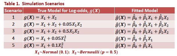
31 A strategy for evaluating goodness-of-fit for a logistic regression model using the Hosmer-Lemeshow test on samples from a large data set Adam Bartley, Michael Pennell, Stanley Lemeshow, and Gary Phillips Purpose of Research Evaluate, through a simulation study, a subsampling approach for assessing goodness-of-fit in large data sets. Use results of simulations to make recommendations for implementing a subsampling approach. Simulation Methods Data were simulated under 5 different scenarios (Table 1). Except for Scenario 1, each data set was analyzed using a model that differed from the truth (Table 1). Scenario 2: true and fitted models were virtually identical. Scenario 4: small difference in the tails. The H-L test was implemented on 100 subsets of size 1,000 and 5,000. Number of significant tests (p-value < 0.05) enumerated. Process repeated for 100 data sets/scenario.

32

33 Results Samples frequently had > 5 significant subsets; even if correct model was fit (Scenario 1). > 20 significant subsets was only common when true and fitted models differed greatly (Scenarios 3 and 5). > 10 subsets uncommon when true and fitted models were the same or almost identical (Scenarios 1, 2). Inadequate power to detect poorly fit models (Scenarios 3 and 5) when subset size < 5,000. True model rejected too often when N < 100,000. Recommendations For N 100,000, draw 100 subsets of size 5,000. Conclude lack-of-fit if H-L test is significant in > 10 subsets.

34 A new calibration test and a reappraisal of the calibration belt for the assessment of prediction models based on dichotomous outcomes Giovanni Nattino, Stefano Finazzi and Guido Bertolini Statistics in Medicine 2014, Recall: ( ) = logit π x logit Pr ( y = 1 x ) ( ( )) = g ( x ) = ˆβ 0 + ˆβ 1 x 1 + ˆβ 2 x 2 +! + ˆβ p x p For each subject, i = 1,2,,n, we can compute: ( x ) i the logit ĝ i the probability ˆπ i = e ( ĝi x i ) ( 1+ e ĝi x i ) Calibration is the agreement between y i and ˆπ i

35 The Calibration Plot

36 The Calibration Plot

37 The Calibration Curve: Now that we ve fit our model, we have for each subject. This relationship can be expressed as { } = α 0 + α 1 logit ˆπ logit Pr ( Y = 1 ˆπ ) ( ) and ĝ i = g x i ˆπ i = Pr y i = 1 x i ( ) { ( )} { ( )} = α 0 + α { 1 ĝ } = logit Pr Y = 1ĝ so, if α 0 = 0 and α 1 = 1 { } = 0 +1 logit ˆπ logit Pr ( Y = 1 ˆπ ) Pr (( Y = 1) ˆπ ) = ˆπ { ( )} = logit ( ˆπ ) If the data fit perfectly, then ˆα 0 0 and ˆα 1 1 but it certainly doesn't have to be a linear relationship

38 Why not: { ( ) ĝ } = α 0 + α 1 ĝ + α 2 ĝ 2 +! + α m ĝ m logit Pr Y = 1 What should we choose for m? if too small too simplistic if too large estimation of useless parameters a forward selection algorithm is used e.g., ICU data m = 2 : logit Pr ( Y = 1) ĝ { } = ĝ ĝ 2 ˆL 2 = m = 3 : logit { Pr ( Y = 1) ĝ } = ĝ ĝ ĝ 3 ˆL 3 = Likelihood Ratio Test: H 0 : α 3 = 0 vs H a : α 3 0 G = , p = NS m = 2

39 so using the m = 2 model: { ( ) ĝ } = ĝ ĝ 2 logit Pr Y = 1 we define the calibration curve as: Pr ( Y = 1 ˆπ ) = f ˆπ ( ) = e logit ˆπ logit ˆπ 1+ e ( )+0.076( logit( ˆπ )) 2 ( ( )) 2 ( ) logit ˆπ

40 so the best model appears to be the m = 2 model: { ( ) ĝ } = ĝ ĝ 2 logit Pr Y = 1 If the calibration were perfect: α 0 = 0, α 1 = 1, α 2 = 0, since then, logit Pr ( Y = 1) ĝ { } = 0 +1 ĝ + 0 = ĝ So we would like to test H 0 : α 0 = 0 and α 1 = 1 and α 2 = 0 vs H a : α 0 0 or α 1 1 or α 2 0 The test: is based on a likelihood ratio statistic; accounts for the iterative process to define m. G = 1.08, p value = Recall: Hosmer-Lemeshow p-value =

41 The calibration belt. calibrationbelt ICU Data Observed Expected

42 Example of a Poorly Calibrated Model:

43 Calibration Belt for this model:

44 So, as we ve seen, the calibration belt can assess the goodness of fit of a model without any categorization. The calibration belt is an informative tool to detect deviations from the perfect fit of a model. The information provided helps improving the goodness of fit of logistic regression models. Let us return to our ongoing modeling efforts.

45 Calibration Belt: Developmental

46 Calibration Belt: Validation

47

48 Thank you!