2: Multiple Linear Regression 2.1
|
|
|
- Geraldine Johnson
- 5 years ago
- Views:
Transcription
1 1. The Model y i = + 1 x i1 + 2 x i2 + + k x ik + i where, 1, 2,, k are unknown parameters, x i1, x i2,, x ik are known variables, i are independently distributed and has a normal distribution with mean 0 and standard deviation, and y i is the value of the response variable for the i th patient. We usually assume that the patient s response y is causally related to the variables x i1, x i2,,x ik through the model. These latter variables are called covariates or explanatory variables; y is called the dependent or response variable. 2: Multiple Linear Regression 2.1
2 2. Reasons for Multiple Linear Regression a) Adjusting for confounding variables To investigate the effect of a variable on an outcome measure adjusted for the effects of other confounding variables. i) 1 estimates the rate of change of y i with x i1 among patients with the same values of x i2, x i3,, x ik. ii) If y i increases rapidly with and x i1, and x i1 and x i2 are highly correlated then the rate of increase of y i with increasing x i1 when x i2 is held constant may be very different from this rate of increase when x i2 is not restrained. 4 y = x 1 + 2x x x NOTE: The model assumes that the rate of change of y i with x i1 adjusted for x i1, x i2,, x ik is the same regardless of the values of these latter variables. 2: Multiple Linear Regression 2.2
3 b) Prediction To predict the value of y given x 1, x 2,, x k 3. Estimating Parameters Let yˆ a bx b x... b x be the estimate of y i given x i1, x i2,, x ik. i 1 i1 2 i2 k ik We estimate a, b 1,, b k by minimizing ( y y ) 2 4. Expected Response in the Multiple Model The expected value of both y i and given her covariates is [ y x ] E[ yˆ x ] x x... x. i i i i 1 i1 2 i2 k ik We estimate the expected value of y i among subjects whose covariate values are identical to those of the i th patient by yˆi. The equation yˆ a bx b x... b x. i 1 i1 2 i2 k ik may be rewritten yˆ y b( x x ) b ( x x )... b ( x x ). {2.1} i i 1 i1 1 2 i2 2 k ik k Thus, yˆ y when x x, x x,..., and x x. yˆi i i1 1 i2 2 ik k 5. Framingham Example: SBP, Age, BMI, Sex and Serum Cholesterol a) Preliminary univariate analysis The Framingham data set contains data on 4,699 patients. On each patient we have the baseline values of the following variables: sbp Systolic blood pressure in mm Hg. age Age in years scl Serum cholesterol in mg/100ml bmi Body mass index in kg/m 2 sex 1 = Men 2 = Women Follow-up information on coronary heart disease is also provided. This data set is a subset of the 40 year data from the Framingham Heart Study that was conducted by the National Heart Lung and Blood Institute. Recruitment of patients started in At that time of the baseline exams there were no effective treatment for hypertension. 2: Multiple Linear Regression 2.3
4 We first perform simple linear regressions of SBP on age, BMI, serum cholesterol.. * FramSBPbmiMulti.log. *. * Framingham data set: Multiple regression analysis of the effect of bmi on. * sbp (Levy 1999).. *. use "c:\wddtext\2.20.framingham.dta", clear. regress sbp bmi Source SS df MS Number of obs = F( 1, 4688) = Model Prob > F = Residual R-squared = Adj R-squared = Total Root MSE = sbp Coef. Std. Err. t P> t [95% Conf. Interval] bmi _cons scatter sbp bmi, symbol(oh) /// > lfit sbp bmi, ytitle(systolic Blood Pressure) Systolic Blood Pressure = Body Mass Index Systolic Blood Pressure Fitted values 2: Multiple Linear Regression 2.4
5 . regress sbp age Source SS df MS Number of obs = F( 1, 4697) = Model Prob > F = Residual R-squared = Adj R-squared = Total Root MSE = sbp Coef. Std. Err. t P> t [95% Conf. Interval] age _cons scatter sbp age, symbol(oh) /// > lfit sbp age, ytitle(systolic Blood Pressure) Systolic Blood Pressure Age in Years = 1.06 Systolic Blood Pressure Fitted values 2: Multiple Linear Regression 2.5
6 . regress sbp scl Source SS df MS Number of obs = F( 1, 4664) = Model Prob > F = Residual R-squared = Adj R-squared = Total Root MSE = sbp Coef. Std. Err. t P> t [95% Conf. Interval] scl _cons scatter sbp scl, symbol(oh) /// > lfit sbp scl, ytitle(systolic Blood Pressure) Systolic Blood Pressure Serum Cholesterol = 0.11 Systolic Blood Pressure Fitted values 2: Multiple Linear Regression 2.6
7 The univariate regressions show that sbp is related to age and scl as well as bmi. Although the statistical significance of the slope coefficients is overwhelming, the R-squared statistics are low. Hence, each of these risk factors individually only explain a modest proportion of the total variability in systolic blood pressure. We would like better understanding of these relationships. Note that the importance of a parameter depends not only on its magnitude but also on the range of the corresponding covariate. For example, the scl coefficient is only 0.11 as compared to 1.83 and 1.06 for bmi and age. However, the range of scl values is from 115 to 568 as compared to for bmi and for age. The large scl range increases the variation in sbp that is associated with scl. Systolic Blood Pressure Age in Years = 1.06 Systolic Blood Pressure Fitted values 2: Multiple Linear Regression 2.7
8 Systolic Blood Pressure Serum Cholesterol = 0.11 Systolic Blood Pressure Fitted values Changing the units of measurement of a covariate can have a dramatic effect on the size of the slope estimate, but no effect on its biologic meaning. For example, suppose we regressed blood pressure against weight in grams. If we converted weight from grams to kilograms we would increase the magnitude of the slope parameter by 1,000 but would have no effect on the true relationship between blood pressure and weight. 2: Multiple Linear Regression 2.8
9 1000 = 1 = Grams Kilograms Density Distribution Sunflower Plots Scatterplots are a simple but informative tool for displaying the relationship between two variables. Their utility decreases when the density of observations makes it difficult to see individual observations. Systolic Blood Pressure Body Mass Index 2: Multiple Linear Regression 2.9
10 A density distribution sunflower plot is an attempt to provide a better sense of a bivariated distribution when observations are densely packed. Data points are represented in one of three ways depending on the density of observations. 1) Low Density: Small circles representing individual data points as in a conventional scatterplot. 2) Medium Density: light sunflowers. 3) High Density: dark sunflowers Diastolic Blood Pressure Diastolic Blood Pressure 1 petal = 1 obs. 1 petal = 6 obs Body Mass Index 2: Multiple Linear Regression 2.10
11 A sunflower is a number of short line segments radiating from a central point. In a light sunflower each petal represents one observation. In a dark sunflower, each petal represents k observations, where k is specified by the user. The x-y plane is divided into a lattice of hexagonal bins. The user can control the bin width in the units of the x-axis and thresholds l and d that determine when light and dark sunflowers are drawn. Whenever there are less than l data points in a bin the individual data points are depicted at their exact location. When there are at least l but fewer than d data points in a bin they are depicted by a light sunflower. When there are at least d observations in a bin they are depicted by a dark sunflower. For more details see the Stata v8.2 online documentation on the sunflower command. 7. Creating Density Distribution Plots with Stata. * FramSunflower.log. *. * Framingham data set: Exploratory analysis of sbp and bmi. *. set more on. use "c:\wddtext\2.20.framingham.dta", clear. * Graphics > Smoothing... > Density-distribution sunflower plot. sunflower sbp bmi {1} Bin width = 1.15 {2} Bin height = {3} Bin aspect ratio = Max obs in a bin = 115 Light = 3 {4} Dark = 13 {5} X-center = 25.2 Y-center = 130 Petal weight = 9 {6} 2: Multiple Linear Regression 2.11
12 {1} Create a sunflower plot of sbp by bmi. Let the program choose all default values. The resulting graph is given in the next slide. {2} The default bin width is given in units of x. It is chosen to provide 40 bins across the graph. {3} The default bin height is given in units of y. It is chosen to make the bins regular hexagons on the graph. {4} The default minimum number of observations in a light sunflower bin is 3 {5} The default minimum number of observations in a dark sunflower bin is 13 {6} The default petal weight for dark sunflowers is chosen so that the maximum number of petals in a dark sunflower is flower petal No. of No. of estimated actual type weight petals flowers obs. obs none light light light light light light light light light light dark dark dark dark dark dark dark dark dark dark dark dark dark : Multiple Linear Regression 2.12

13 Systolic Blood Pressure Body Mass Index Systolic Blood Pressure 1 petal = 9 obs. 1 petal = 1 obs. 2: Multiple Linear Regression 2.13
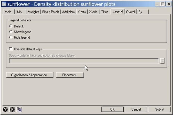
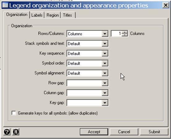
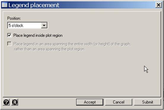
14 . more. * Graphics > Smoothing... > Density-distribution sunflower plot. sunflower dbp bmi, binwidth(0.85) /// {1} > ylabel(50 (20) 150, angle(0)) ytick(40 (5) 145) /// > xlabel(20 (5) 55) xtick(16 (1) 58) /// > legend(position(5) ring(0) cols(1)) /// {2} > addplot(lfit dbp bmi, color(green) /// {3} > lowess dbp bmi, bwidth(.2) color(cyan) ) Bin width =.85 Bin height = Bin aspect ratio = Max obs in a bin = 59 Light = 3 Dark = 13 X-center = 25.2 Y-center = 80 Petal weight = 5 {1} sunflower accepts most standard graph options as well as special options that can control almost all aspects of the plot. Here binwidth specifies the bin width to be 0.85 kg/m 2. {2} The position sub-option of the legend option specifies that the legend will be located at 5 o clock. ring(0) causes the legend to be drawn within the graph region. cols(1) requires that the legend keys be in a single column. {3} The addplot option allows us to overlay other graphs on top of the sunflower plot. Here we draw the linear regression and lowess regression curves. 2: Multiple Linear Regression 2.14

15 2: Multiple Linear Regression 2.15

16 2: Multiple Linear Regression 2.16
17 Diastolic Blood Pressure/Fitted values/lowess dbp bmi Diastolic Blood Pressure 1 petal = 1 obs. 1 petal = 5 obs. Fitted values lowess dbp bmi Body Mass Index 8. Scatterplot matrix graphs Another useful exploratory graphic is the scatter plot matrix. Here we look at the combined marginal effects of sbp age bmi and scl. The graph is restricted to women recruited in January to reduce the number of data points. FramSBPbmiMulti.log continues as follows. * Graphics > Scatterplot matrix. graph matrix sbp bmi age scl if month==1 & sex==2,msymbol(oh) {1} {1} The matrix option generates a matrix scatter plot for sbp bmi age and scl. The if clause restricts the graph to women (sex==2) who entered the study in January (month==1). oh specifies a small hollow circle as a plot symbol 2: Multiple Linear Regression 2.17


18 This graphic shows all 2x2 scatter plots of the specified variables Systolic Blood Pressure Body Mass Index Age in Years Serum Cholesterol : Multiple Linear Regression 2.18
19 9. Modeling interaction in the Framingham baseline data The first model that comes to mind is [ sbp x ] bmi age scl sex. i i 1 i 2 i 3 i 4 i A potential weakness of this model is that it implies that the effects of the covariates on sbp i are additive. To understand what this means, suppose we hold age and scl constant and look at bmi and sex. Then the model becomes sbp = constant + bmi x for men, and sbp = constant + bmi x for women. The 4 parameter allows men and women with the same bmi to have different expected sbps. However, the slope of the sbp-bmi relationship for both men and women is 1. Interaction No Interaction We know, however, that this slope is higher for women than for men. This is an example of what we call interaction in which the effect of one variate on the dependent variable is influenced by the value of a second covariate. 2: Multiple Linear Regression 2.19
20 We need a more complex model to deal with interaction. Let women = sex -1. Then women = Consider the model sbp = 1 + bmi x 2 + women x 3 + bmi x women x 4 This model reduces to sbp = 1 + bmi x 2 for men and 1: if subject is female 0: if subject is male sbp = 1 + bmi x ( ) + 3 for women. Hence 4 estimates the difference in slopes between men and women. Interaction No Interaction We use this approach to build an appropriate multivariate model for the Framingham data. FramSBPbmiMulti.log continues as follows.. *. * Use multiple regression models with interaction terms to analyze. * the effects of sbp, bmi, age and scl on sbp.. *. generate woman = sex - 1. label define truth 0 "False" 1 "True". label values woman truth. generate bmiwoman = bmi*woman (9 missing values generated). generate agewoman = age*woman. generate sclwoman = woman * scl (33 missing values generated) 2: Multiple Linear Regression 2.20
21 . regress sbp bmi age scl woman bmiwoman agewoman sclwoman Source SS df MS Number of obs = F( 7, 4650) = Model Prob > F = Residual R-squared = {1} Adj R-squared = Total Root MSE = sbp Coef. Std. Err. t P> t [95% Conf. Interval] bmi age scl woman bmiwoman agewoman sclwoman {2} _cons {1} R-squared equals the square of the correlation coefficient between 2 2 yˆi and yi. It still equals ( yˆi y ) / ( yi y ) and hence can be interpreted as the proportion of the variation in y explained by the model. In the simple regression of sbp and bmi we had R-squared = Thus, this multiple regression model explains more than twice the variation in sbp than did the simple model. {2} The serum cholesterol-woman interaction coefficient, , is five times smaller than the scl coefficient, and is not statistically significant. Lets drop it from the model and see what happens. 2: Multiple Linear Regression 2.21

22 . regress sbp bmi age scl woman bmiwoman agewoman Source SS df MS Number of obs = F( 6, 4651) = Model Prob > F = Residual R-squared = {3} Adj R-squared = Total Root MSE = sbp Coef. Std. Err. t P> t [95% Conf. Interval] bmi age scl woman bmiwoman {4} agewoman _cons {3} Dropping the sclwoman term has a trivial effect on the R-squared statistic and little effect on the model coefficients. {4} The bmiwoman interaction term is also not significant and is an order of magnitude smaller than the bmi term. Lets drop it. 2: Multiple Linear Regression 2.22
23 . regress sbp bmi age scl woman agewoman Source SS df MS Number of obs = F( 5, 4652) = Model Prob > F = Residual R-squared = {5} Adj R-squared = Total Root MSE = sbp Coef. Std. Err. t P> t [95% Conf. Interval] bmi age scl woman agewoman _cons {5} Dropping the preceding term reduces the R 2 value by 0.04%. The remaining terms are highly significant. When we did simple linear regression of sbp against bmi for men and women we obtained slope estimates of 1.38 and 2.05 for men and women, respectively. Our multivariate model gives a single slope estimate of 1.36 for both sexes, but finds that the effect of increasing age on sbp is twice as large in women than men. I.e. For women this slope is = 1.18 while for men it is How reasonable is our model? One way to increase our intuitive understanding of the model is to plot separate simple linear regressions of sbp against bmi in groups of patients who are homogeneous with respect to the other variables in the model. The following graphic is restricted to patients with a serum cholesterol of < 225 and subdivides patients by age and sex. In these graphs, two versions of the graph are given drawn to different scales. The second only shows the regression lines. 2: Multiple Linear Regression 2.23
24 Men Women Systolic Blood Pressure < Age < < Age < Systolic Blood Pressure < Age < < Age < Systolic Blood Pressure < Age < < Age < Systolic Blood Pressure < Age < < Age < Body Mass Index Body Mass Index The blue lines have the slope from our multiple regression model of 1.36 The red lines have slopes 1.38 for men and 2.05 for women (the slopes of the simple regressions in men and women respectively. The green lines have the slope of the simple regression for patients with the indicated age and gender. The yellow lines mark the mean sbp and bmi for the indicated age-gender group. 2: Multiple Linear Regression 2.24
25 Systolic Blood Pressure Systolic Blood Pressure Systolic Blood Pressure Systolic Blood Pressure < Age < < Age < < Age < < Age < 40 Men 60 < Age < < Age < < Age < 50 Women 30 < Age < Body Mass Index Body Mass Index For men the adjusted and unadjusted slopes are almost identical and are very close to the age restricted slope for all ages except However, for women the adjusted and unadjusted slopes differ appreciably. The adjusted slope is very close to the age restricted slopes in every case except age 60-70, where the adjusted slope is closed the age restricted slope than is the unadjusted slope. Thus, our model is a marked improvement over the simple model. The single sbp-bmi adjusted slope estimate appears reasonable except, for the oldest subjects. Note that the mean sbp increases with age for both sexes, but increases more rapidly in women than in men. The mean bmi does not vary appreciably with age in men but does increase with increasing age in women. Thus age and gender confound the effect of bmi on sbp. Do you think that the age-gender interaction of sbp is real or is this driven by some other unknown confounding variable? 2: Multiple Linear Regression 2.25
26 10. Automatic Methods of Model Selection Analyses loose power when we include variables in the model that are neither confounders nor variables of interest. When a large number of potential confounders are available it can be useful to use an automatic model selection program. a) Forward Selection i) Fit all simple linear models of y against each separate x variable. Select the variable with the greatest significance. ii) Fit all possible models with the variable(s) selected in the preceding step(s) and one other. Select as the next variable the one with the greatest significance among these models. iii) repeat step ii) to add additional variables, one variable at a time. Continue this process until none of the remaining variables have a significance level less than some threshold. We next illustrate how this is done in Stata. FramSBPbmiMulti.log continues as follows.. *. * Fit a model of sbp against bmi age scl and sex with. * interaction terms. The variables woman, bmiwoman,. * agewoman, and sclwoman have been previously defined.. *. * statistics > other > stepwise estimation. stepwise, pe(.1): regress sbp bmi age scl woman bmiwoman agewoman sclwoman {1} begin with empty model p = < adding age {2} p = < adding bmi {3} p = < adding scl p = < adding agewoman p = < adding woman Source SS df MS Number of obs = F( 5, 4652) = Model Prob > F = Residual R-squared = Adj R-squared = Total Root MSE = 19.8 sbp Coef. Std. Err. t P> t [95% Conf. Interval] age bmi scl agewoman woman _cons : Multiple Linear Regression 2.26

27 {1} Fit a model using forward selection; pe(.1) means that the P value for entry is 0.1. At each step new variables will only be considered for entry into the model if their P value after adjustment for previously entered variables is <0.1. {2} In the first step the program considers the following models. sbp = 1 + bmi x 2 sbp = 1 + age x 2 sbp = 1 + scl x 2 sbp = 1 + woman x 2 sbp = 1 + bmiwoman x 2 sbp = 1 + agewoman x 2 sbp = 1 + sclwoman x 2 Of these models the one with age has the most significant slope parameter. The P value associated with this parameter is <0.1. Therefore we select age and go on to step 2. {3} In step 2 we consider the models sbp = 1 + age x 2 + bmi x 3 sbp = 1 + age x 2 + scl x 3 sbp = 1 + age x 2 + sclwoman x 3 2: Multiple Linear Regression 2.27
28 The most significant new term in these models is bmi, which is selected. This process is continued until at the end of step 5 we have the model sbp 1 age 2 bmi 3 scl 4 agewoman woman 5 6 In step 6 we consider the models sbp 1 age 2 bmi 3 scl 4 agewoman woman bmiwoman and sbp 1 age 2 bmi 3 scl 4 agewoman woman sclwoman However, neither of the P values for the 7 parameter estimates in these models are < 0.1. Therefore, neither of these terms are added to the model.. *. * Fit a model of sbp against bmi age scl and sex with. * interaction terms. The variables woman, bmiwoman,. * agewoman, and sclwoman have been previously defined.. *. * statistics > other > stepwise estimation. stepwise, pe(.1): regress sbp bmi age scl woman bmiwoman agewoman sclwoman begin with empty model p = < adding age p = < adding bmi p = < adding scl p = < adding agewoman p = < adding woman Source SS df MS Number of obs = F( 5, 4652) = Model Prob > F = Residual R-squared = Adj R-squared = Total Root MSE = 19.8 sbp Coef. Std. Err. t P> t [95% Conf. Interval] age bmi scl agewoman woman _cons : Multiple Linear Regression 2.28

29 b) Backward Selection This method is similar to the forward method except that we start with all the variables and eliminate the variable with the least significance. The data is refit with the remaining variables and the process is repeated until all remaining variables have a significance level below some threshold. The Stata command to use backward selection for our sbp example is. * statistics > other > stepwise estimation. stepwise, pr(.1): regress sbp bmi age scl woman bmiwoman > agewoman sclwoman, Here pr(.1) means that the program will consider variables for removal from the model if their associated P value is > 0.1. If you run this command in this example you will get the same answer as with the forward selection, which is reassuring. In general there is no guarantee that this will happen. 2: Multiple Linear Regression 2.29
30 c) Stepwise Selection This method is like the forward method except that at each step, previously selected variables whose significance has dropped below some threshold are dropped from the model. Suppose: x 1 is the best single predictor of y x 2 and x 3 are chosen next and together predict y better than x 1 Then it makes sense to keep x 2 and x 3 and drop x 1 from the model. In the Stata stepwise command this is done with the options -,forward pe(.1) pr(.2) which would consider new variables for selection with P < 0.1 and previously selected variables for removal with P > Pros and cons of automated model selection i) Automatic selection methods are fast and easy to use. ii) iii) iv) They are best used when we have a small number of variables of primary interest and wish to explore the effects of potential confounding variables on our models. They can be misleading when used for exploratory analyses in which the primary variables of interest are unknown and the number of potential covariates is large. In this case these methods can exaggerate the importance of a small number of variables due to multiple comparisons artifacts. It is a good idea to use more than one method to see if you come up with the same model. v) Fitting models by hand may sometimes be worth the effort. 2: Multiple Linear Regression 2.30
31 12. Residuals, Leverage, and Influence a) Residuals The residual for the i th patient is e y yˆ i i i b) Estimating the variance 2 We estimate 2 by s 2 = (y i - ŷi) 2 /(n - k - 1) {2.2} which is denoted Mean Square for Error in most computer programs. In Stata it is the term in the Residual row and the MS column. k is the number of covariates in the model.. regress sbp bmi age scl woman agewoman Source SS df MS Number of obs = F( 5, 4652) = Model Prob > F = Residual R-squared = Adj R-squared = Total Root MSE = sbp Coef. Std. Err. t P> t [95% Conf. Interval] bmi age scl woman agewoman _cons : Multiple Linear Regression 2.31
32 c) Leverage The leverage h i of the i th patient is a measure of her potential to influence the parameter estimates if the i th residual is large. h i has a complex formula involving the covariates x 1, x 2,, x k (but not the dependent variable y). In all cases 0 < h i < 1. The larger h i the greater the leverage. The variance of y i is 2 i var( y ) hs. ˆi h 2 Note that var y / s. i ˆi Hence h can be defined as the variance of y measured in units of s. i ˆi 2 d) Residual variance The variance of e i is s 2 (1 h i ) e) Standardized and Studentized residual The standardized residual is r e /( s 1 h ) {2.3} i i i The studentized residual is t e /( s 1 h i ) {2.4} i i () i where s (i) is the estimate of obtained from equation (2.2) with the i th case deleted (t i is also called the jackknifed residual). It is often helpful to plot the studentized residual against its expected value. We do this in Stata as we continue the session recorded in FramSBPbmiMulti.log. 2: Multiple Linear Regression 2.32
33 . predict yhat, xb (41 missing values generated). predict res, rstudent. * Statistics > Nonparametric analysis > Lowess smoothing. lowess res yhat, bwidth(0.2) symbol(oh) color(gs10) lwidth(thick) /// > yline( ) ylabel(-2 (2) 6) ytick(-2 (1) 6) /// > xlabel(100 (20) 180) xtitle(expected SBP) Lowess smoother Studentized residuals Expected SBP bandwidth =.2 2: Multiple Linear Regression 2.33
34 If our model fit perfectly, the lowess regression line would be flat and equal to zero, 95% of the studentized residuals would lie between + 2 and should be symmetric about zero. In this example the residuals are skewed but the regression line keeps close to zero except for very low values of expected SBP. Thus, this graph supports the validity of the model with respect to the expected SBP values but not with respect to the distribution of the residuals. The very large sample size, however, should keep the non-normally distributed residuals from adversely affecting our conclusions. f) Influence The influence of a patient is the extent to which he determines the value of the regression coefficients. 13. Cook's Distance: Detecting Multivariate Outliers One measure of influence is Cook s distance, D i, which is a function of r i and h i. The removal of a patient with a D i value greater than 1 shifts the parameter estimates outside the 50% confidence region based on the entire data set. Checking observations with a Cook s distance greater than 0.5 is worthwhile. Such observations should be double checked for errors. If they are valid you may need to discuss them explicitly in you paper. It is possible for a multivariate outlier to have a major effect on the parameter estimates but not be an obvious outlier on a 2 2 scatter plot. 2: Multiple Linear Regression 2.34
. We illustrate the influence of individual patients in a subset analysis of subjects with IDs from 2001 to 2050. FramSBPbmiMulti.log continues as follows.. *.")
35 14. Cook s Distance in the SBP Regression Example The Framingham data set is so large that no individual observation has an appreciable effect on the parameter estimates (the maximum Cook s distance is 0.009). We illustrate the influence of individual patients in a subset analysis of subjects with IDs from 2001 to FramSBPbmiMulti.log continues as follows.. *. * Illustrate influence of individual data points on. * the parameter estimates of a linear regression.. *. * Variables Manager (right click on variable to be dropped or kept). drop res * Data > Create or change data > Keep or drop observations. keep if id > 2000 & id <= 2050 (4649 observations deleted). regress sbp bmi age scl woman agewoman, level(50) {1} {1} The level(50) option specifies that 50% confidence intervals will be given for the parameter estimates. 2: Multiple Linear Regression 2.35
36 Source SS df MS Number of obs = F( 5, 43) = 2.13 Model Prob > F = Residual R-squared = Adj R-squared = Total Root MSE = sbp Coef. Std. Err. t P> t [50% Conf. Interval] bmi age scl woman agewoman _cons predict res, rstudent (1 missing value generated). predict cook, cooksd {2} (1 missing value generated) {2} Define cook to equal the Cook s distance for each data point.. label variable res "Studentized Residual". label variable cook "Cook's Distance". scatter cook res, ylabel(0 (.1).5) xlabel(-2 (1) 5) Cook's Distance Studentized Residual The graph shows that we have one enormous residual with great influence. Note however that there are also large residuals with little influence. 2: Multiple Linear Regression 2.36
37 The log file continues as follows:. list cook res id bmi sbp if res > 2 cook res id bmi sbp {1}. regress sbp bmi age scl woman agewoman if id ~= 2049, level(50) {2} Source SS df MS Number of obs = F( 5, 42) = 2.83 Model Prob > F = Residual R-squared = Adj R-squared = Total Root MSE = sbp Coef. Std. Err. t P> t [50% Conf. Interval] bmi {3} age scl woman agewoman _cons {1} The patient with the large Cook s D has ID {2} We repeat the linear regression excluding this patient. {3} Excluding this one patient increases the bmi coefficient from to 1.78, which exceeds the upper bound of the 50% confidence interval for bmi from the initial regression. 2: Multiple Linear Regression 2.37
38 . regress sbp bmi age scl woman agewoman, level(50) Source SS df MS Number of obs = F( 5, 43) = 2.13 Model Prob > F = Residual R-squared = Adj R-squared = Total Root MSE = sbp Coef. Std. Err. t P> t [50% Conf. Interval] bmi age scl woman agewoman _cons The following graph shows a scatter plot of sbp by bmi for these 50 patients. The red and blue lines have slopes of 1.78 and 0.516, respectively (the lines are drawn through the mean sbp and bmi values). Patients 2048 and 2049 are indicated by arrows. The influence of patient 2048 is greatly reduced by thefactthathisbmi of 24.6 is near the mean bmi. The influence of patient 2049 is not only affected by her large residual but also by her low bmi that exerts leverage on the regression slope. Systolic Blood Pressure 250 Enormous residual with great influence < id < 2051 Large residual with little influence Body Mass Index 2: Multiple Linear Regression 2.38
39 15. Least Squares Estimation In simple linear regression we have introduced the concept of estimating parameters by the method of least squares. We chose a model of the form E(y i ) = + x i. We estimated by a and by b letting y = a + bx and then choosing a and b so as to minimize the sum of squared residuals y yˆ 2 This approach works well for linear regression. It is ineffective for some other regression methods Another approach which can be very useful is maximum likelihood estimation 16. Maximum Likelihood Estimation In simple linear regression we observed pairs of observations y, x : i 1,2,, n i i and fit the model E(y i ) = + x i We calculate the likelihood function L, y, x : i 1,2,, n {1} i i which is the probability of obtaining the observed data given the specified value of and. The maximum likelihood estimates of and are those values of these parameters that maximize equation {1} In linear regression the maximum likelihood and least squares estimates of and are identical. 2: Multiple Linear Regression 2.39
40 17. Information Criteria for Assessing Statistical Models We seek models that fit the data well are simple will be useful for future data Increasing the number of parameters will improve the fit to the current data increase model complexity may exaggerate findings We often must choose between a number of competing models. We seek measures of model fit that take into account both how well the data fit the model and the complexity of the model. Suppose we have a model with k parameters and n observations. Let L be the maximum value of the likelihood function for this model. Then Akaike s Information Criteria AIC = 2 log e L + 2k Schwarz s Bayesian Information Criteria BIC = 2 log e L + k log e n Models with lower values of AIC or BIC are usually preferred over models with higher values of these statistics. Models that fit well will have higher values of L and hence lower values of 2 log e L. Smaller models have smaller values of k and hence give lower AIC and BIC values. For studies with more than 8 patients, BIC gives a higher penalty per parameter than AIC. There are theoretical justifications for both methods. Neither is clearly better than the other. 2: Multiple Linear Regression 2.40

41 18. Using Multiple Linear Regression for Non-linear Models Multiple linear regression can be used to build simple non-linear models. For example, suppose that there was a quadratic relationship between an independent variable x and the expected value of y. Then we could use the model y x x {2.5} 2 i 1 i 2 i i 6 y y x x E 1 2 i i i x The preceding models E y i as a non-linear function of xi. It is fine when correct but performs poorly for many non-linear models where the x-y relationship is not quadratic. Extrapolating from this model is particularly problematic. 6 4 y y x x E 1 2 i i i x 2: Multiple Linear Regression 2.41
42 Note that {2.5} is a linear function of the parameters. Hence, it is a multiple linear regression model even though it is nonlinear in xi We seek a more flexible approach to building non-linear regression models using multiple linear regression models. 6 y x x 2 i 1 i 2 i i 4 y x 19. Restricted Cubic Splines We wish to model y i as a function of x i using a flexible non-linear model. In a restricted cubic spline model we introduce k knots on the x-axis located at t1, t2,, t k. We select a model of the expected value of y that is linear before t and after t. 1 k consists of piecewise cubic polynomials between adjacent knots 3 2 (i.e. of the form ax bx cx d ) is continuous and smooth at each knot. (More technically, its first and second derivatives are continuous at each knot.) An example of a restricted cubic spline with three knots is given on the next slide. 2: Multiple Linear Regression 2.42
43 t t t Example of a restricted cubic spline with three knots Given x and k knots, a restricted cubic spline can be defined by y x x x k 1 k 1 for suitably defined values of These covariates are functions of x and the knots but are independent of y. xi x1 x and hence the hypothesis k tests the linear hypothesis If x is less than the first knot then x x xk This fact will prove useful in survival analyses when calculating relative risks Programs to calculate x1,, xk 1are available in Stata, R and other statistical software packages. The functional definitions of these terms are not pretty (see Harrell 2001), but this is of little concern given programs that will calculate them for you. Users can specify the knot values. However, it is often reasonable to let you program choose them for you. 2: Multiple Linear Regression 2.43
44 Harrell (2001) recommends placing knots at the quantiles of the x variable given in the following table Number of knots k Knot locations expressed in quantiles of the x variable The basic idea of this table is to place t 1 and t k near the extreme values of x and to space the remaining knots so that the proportion of observations between knots remains constant. When there are fewer than 100 data points Harrell recommends replacing the smallest and largest knots by the fifth smallest and fifth largest observation, respectively. The choice of number of knots involves a trade-off between model flexibility and number of parameters. Stone (1986) has found that more than 5 knots are rarely needed to obtain a good fit. Five knots is a good choice when there are at least 100 data points. Using fewer knots makes sense when there are fewer data points It is important to always do a residual plot or, at a minimum, plot the observed and expected values to ensure that you have obtained a good fit. The linear fits beyond the largest and smallest knots usually tracks the data well, but is not guaranteed to do so. 2: Multiple Linear Regression 2.44
45 20. Example: the SUPPORT Study A prospective observational study of hospitalized patients Lynn & Knauss: "Background for SUPPORT." J Clin Epidemiol 1990; 43: 1S - 4S. A random sample of data from 996 subjects in this study is available. See SUPPORT.dta los = length of stay in days. map = baseline mean arterial pressure fate = 1: Patient died in hospital 0: Patient discharged alive Length of Stay (days) Mean Arterial Pressure (mm Hg) 2: Multiple Linear Regression 2.45
46 21. Fitting a Restricted Cubic Spline with Stata. * SupportLinearRCS.log. *. * Draw scatter plots of length-of-stay (LOS) by mean arterial. * pressure (MAP) and log LOS by MAP for the SUPPORT Study data. * (Lynn & Knauss, 1990).. *. use "C:\WDDtext\ SUPPORT.dta", replace. scatter los map, symbol(oh) xlabel(25 (25) 175) xmtick(20 (5) 180) /// {1} > ylabel(0(25)225, angle(0)) ymtick(5(5)240) {1} Length of stay is highly skewed. Length of Stay (days) Mean Arterial Pressure (mm Hg) 2: Multiple Linear Regression 2.46
90) {2} Plotting log LOS makes the distribution of this variable more normal. The yscale(log) option does this tranformation.")
47 . scatter los map, symbol(oh) xlabel(25 (25) 175) xmtick(20 (5) 180) /// > yscale(log) ylabel(4(2)10 20(20) , angle(0)) /// {2} > ymtick(3(1)9 30(10)90) {2} Plotting log LOS makes the distribution of this variable more normal. The yscale(log) option does this tranformation. 2: Multiple Linear Regression 2.47
48 200 Length of Stay (days) Mean Arterial Pressure (mm Hg). *. * Regress log LOS against MAP using RCS models with. * 5 knots at their default locations. Overlay the expected. * log LOS from these models on a scatter plot of log LOS by MAP.. *. * Data > Create... > Other variable-creation... > linear and cubic... mkspline _Smap = map, cubic displayknots {1} knot1 knot2 knot3 knot4 knot map {1} The mkspline command generates either linear or restricted cubic spline covariates. The cubic option specifies that restricted cubic spline covariates are to be created. This command generates these covariates for the variable map. By default, 5 knots are used at their default locations. Following Harrell's recommendation the computer places them at the 5th, 27.5 th, 50 th, 72.5th and 95th percentiles of map. The values of these knots are listed. The 4 spline covariates associated with these 5 knots are named _Smap1 _Smap2 _Smap3 _Smap4 These names are obtained by concatenating the name _Smap given before the equal sign with the numbers 1, 2, 3 and 4. 2: Multiple Linear Regression 2.48

49 . summarize _Smap1 _Smap2 _Smap3 _Smap4 {2} Variable Obs Mean Std. Dev. Min Max _Smap _Smap _Smap _Smap {2} _Smap1 is identical to map. The other spline covariates take nonnegative values. 2: Multiple Linear Regression 2.49
50 . generate log_los = log(los). regress log_los _S* {3} Source SS df MS Number of obs = F( 4, 991) = Model Prob > F = Residual R-squared = Adj R-squared = Total Root MSE = log_los Coef. Std. Err. t P> t [95% Conf. Interval] _Smap _Smap _Smap _Smap _cons {3} This command regresses log_los against all variables that start with the characters _S. The only variables with these names are the spline covariates. An equivalent way of running this regression would be regress log_los _Smap1 _Smap2 _Smap3 _Smap4. generate log_los = log(los). regress log_los _S* Source SS df MS Number of obs = F( 4, 991) = {4} Model Prob > F = Residual R-squared = Adj R-squared = Total Root MSE = log_los Coef. Std. Err. t P> t [95% Conf. Interval] _Smap _Smap _Smap _Smap _cons {4} This F statistic tests the null hypothesis that the coefficients associated with the parameters of the spline covariates are simultaneously zero. In other words, it tests the hypothesis that length of stay is unaffected by MAP. It is significant with P < : Multiple Linear Regression 2.50
 ll(model) df AIC BIC")
51 * Statistics > Postestimation > Reports and statistics. estat ic {5} Model Obs ll(null) ll(model) df AIC BIC Note: N=Obs used in calculating BIC; see [R] BIC note {5} Calculate the AIC and BIC for this model.. * Statistics > Postestimation > Tests > Test linear hypotheses. test _Smap2 _Smap3 _Smap4 {6} ( 1) _Smap2 = 0 ( 2) _Smap3 = 0 ( 3) _Smap4 = 0 F( 3, 991) = Prob > F = {6} Test the null hypothesis that there is a linear relationship between map and log_los. Since _Smap1 = map, this is done by testing the null hypothesis that the coefficients associated with _Smap2, _Smap3 and _Smap4 are all simultaneously zero. This test is significant with P < : Multiple Linear Regression 2.51
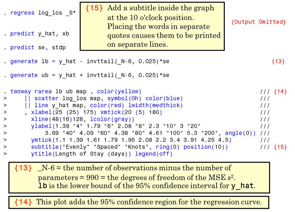
 /// {8} > line y_hat5 map, color(red) lwidth(medthick) /// >, xlabel(25 (25) 175) xmtick(20 (5) 180) /// > xline(47 66 78 106 129, lcolor(blue)) /// {9} > ylabel(1.")
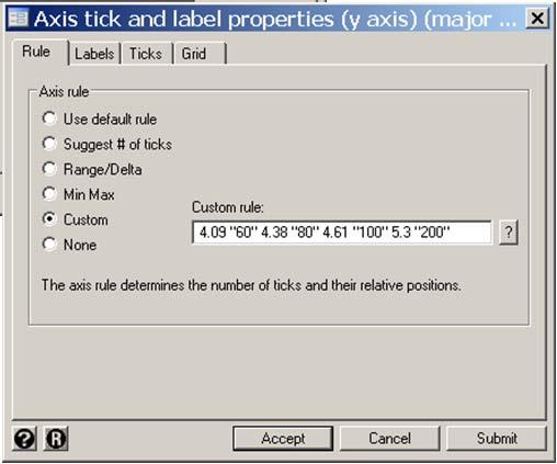
52 {7} y_hat is the estimated expected value of log_los under this model.. predict y_hat5, xb {7}. scatter log_los map, symbol(oh) /// {8} > line y_hat5 map, color(red) lwidth(medthick) /// >, xlabel(25 (25) 175) xmtick(20 (5) 180) /// > xline( , lcolor(blue)) /// {9} > ylabel(1.39 "4" 1.79 "6" 2.08 "8" 2.3 "10" 3 "20" /// {10} > 3.69 "40" 4.09 "60" 4.38 "80" 4.61 "100" 5.3 "200", angle(0)) /// > ymtick( ) /// > ytitle(length of Stay (days)) /// > legend(order(1 "Observed" 2 "Expected")) {8} Graph a scatterplot of log_los vs. map together with a line plot of the expected log_los vs. map. {9} This xline option draws vertical lines at each of the five knots. The lcolor suboption colors these lines blue. {10} The units of the y-axis is length of stay. This ylabel option places the label 4 at the y-axis value 1.39 = log(4), 6 at the value 1.79 = log(6), etc. 2: Multiple Linear Regression 2.52

53 2: Multiple Linear Regression 2.53
54 200 Length of Stay (days) Mean Arterial Pressure (mm Hg) Observed Expected. *. * Plot expected LOS for models with 3, 4, 6 and 7 knots.. * Use the default knot locations. Calculate AIC and BIC for each model.. *. * Variables Manager. drop _S*. * Data > Create... > Other variable-creation... > linear and cubic.... mkspline _Smap = map, nknots(3) cubic displayknots {11} knot1 knot2 knot map {11} Define 2 spline covariates associated with 3 knots at their default locations. The nknots option specifies the number of knots. 2: Multiple Linear Regression 2.54

![Interval] -------------+---------------------------------------------------------------- _Smap1 -.0110138.0027449-4.01 0.000 -.0164002 -.0056274 _Smap2.0226496.004248 5.33 0.000.0143135.](/docs-images/86/94330482/images/55-1.jpg "0309858 _cons 3.124095.1827706 17.09 0.000 2.765435 3.482756. predict y_hat3, xb.")
55 . regress log_los _S* Source SS df MS Number of obs = F( 2, 993) = Model Prob > F = Residual R-squared = Adj R-squared = Total Root MSE =.8078 log_los Coef. Std. Err. t P> t [95% Conf. Interval] _Smap _Smap _cons predict y_hat3, xb. estat ic Model Obs ll(null) ll(model) df AIC BIC Note: N=Obs used in calculating BIC; see [R] BIC note 2: Multiple Linear Regression 2.55
56 . drop _S*. mkspline _Smap = map, nknots(4) cubic displayknots knot1 knot2 knot3 knot map regress log_los _S* Source SS df MS Number of obs = F( 3, 992) = Model Prob > F = Residual R-squared = Adj R-squared = Total Root MSE = log_los Coef. Std. Err. t P> t [95% Conf. Interval] _Smap _Smap _Smap _cons predict y_hat4, xb. estat ic Model Obs ll(null) ll(model) df AIC BIC Note: N=Obs used in calculating BIC; see [R] BIC note. drop _S*. mkspline _Smap = map, nknots(6) cubic displayknots knot1 knot2 knot3 knot4 knot5 knot map : Multiple Linear Regression 2.56
57 . regress log_los _S* Source SS df MS Number of obs = F( 5, 990) = Model Prob > F = Residual R-squared = Adj R-squared = Total Root MSE = log_los Coef. Std. Err. t P> t [95% Conf. Interval] _Smap _Smap _Smap _Smap _Smap _cons predict y_hat6, xb. estat ic Model Obs ll(null) ll(model) df AIC BIC Note: N=Obs used in calculating BIC; see [R] BIC note 2: Multiple Linear Regression 2.57
58 200 Length of Stay (days) knots 4 knots 5 knots 6 knots 7 knots Mean Arterial Pressure (mm Hg) 2: Multiple Linear Regression 2.58

59 2: Multiple Linear Regression 2.59

60 2: Multiple Linear Regression 2.60
 100")


61 200 Evenly Spaced Knots Length of Stay (days) Mean Arterial Pressure (mm Hg) 2: Multiple Linear Regression 2.61
62 200 Default Knot Values Length of Stay (days) Mean Arterial Pressure (mm Hg) 2: Multiple Linear Regression 2.62


63 2: Multiple Linear Regression 2.63


64 2: Multiple Linear Regression 2.64
STATISTICS 110/201 PRACTICE FINAL EXAM
 STATISTICS 110/201 PRACTICE FINAL EXAM Questions 1 to 5: There is a downloadable Stata package that produces sequential sums of squares for regression. In other words, the SS is built up as each variable
Correlation and Simple Linear Regression
 Correlation and Simple Linear Regression Sasivimol Rattanasiri, Ph.D Section for Clinical Epidemiology and Biostatistics Ramathibodi Hospital, Mahidol University E-mail: sasivimol.rat@mahidol.ac.th 1 Outline
1 A Review of Correlation and Regression
 1 A Review of Correlation and Regression SW, Chapter 12 Suppose we select n = 10 persons from the population of college seniors who plan to take the MCAT exam. Each takes the test, is coached, and then
Linear Modelling in Stata Session 6: Further Topics in Linear Modelling
 Linear Modelling in Stata Session 6: Further Topics in Linear Modelling Mark Lunt Arthritis Research UK Epidemiology Unit University of Manchester 14/11/2017 This Week Categorical Variables Categorical
Topic 18: Model Selection and Diagnostics
 Topic 18: Model Selection and Diagnostics Variable Selection We want to choose a best model that is a subset of the available explanatory variables Two separate problems 1. How many explanatory variables
General Linear Model (Chapter 4)
") General Linear Model (Chapter 4) Outcome variable is considered continuous Simple linear regression Scatterplots OLS is BLUE under basic assumptions MSE estimates residual variance testing regression coefficients
General Linear Model (Chapter 4) Outcome variable is considered continuous Simple linear regression Scatterplots OLS is BLUE under basic assumptions MSE estimates residual variance testing regression coefficients
Acknowledgements. Outline. Marie Diener-West. ICTR Leadership / Team INTRODUCTION TO CLINICAL RESEARCH. Introduction to Linear Regression
 INTRODUCTION TO CLINICAL RESEARCH Introduction to Linear Regression Karen Bandeen-Roche, Ph.D. July 17, 2012 Acknowledgements Marie Diener-West Rick Thompson ICTR Leadership / Team JHU Intro to Clinical
Soc 63993, Homework #7 Answer Key: Nonlinear effects/ Intro to path analysis
 Soc 63993, Homework #7 Answer Key: Nonlinear effects/ Intro to path analysis Richard Williams, University of Notre Dame, https://www3.nd.edu/~rwilliam/ Last revised February 20, 2015 Problem 1. The files
Statistical Modelling in Stata 5: Linear Models
 Statistical Modelling in Stata 5: Linear Models Mark Lunt Arthritis Research UK Epidemiology Unit University of Manchester 07/11/2017 Structure This Week What is a linear model? How good is my model? Does
171:162 Design and Analysis of Biomedical Studies, Summer 2011 Exam #3, July 16th
 Name 171:162 Design and Analysis of Biomedical Studies, Summer 2011 Exam #3, July 16th Use the selected SAS output to help you answer the questions. The SAS output is all at the back of the exam on pages
Lecture 3: Multiple Regression. Prof. Sharyn O Halloran Sustainable Development U9611 Econometrics II
 Lecture 3: Multiple Regression Prof. Sharyn O Halloran Sustainable Development Econometrics II Outline Basics of Multiple Regression Dummy Variables Interactive terms Curvilinear models Review Strategies
Sociology Exam 2 Answer Key March 30, 2012
 Sociology 63993 Exam 2 Answer Key March 30, 2012 I. True-False. (20 points) Indicate whether the following statements are true or false. If false, briefly explain why. 1. A researcher has constructed scales
Sociology 63993, Exam 2 Answer Key [DRAFT] March 27, 2015 Richard Williams, University of Notre Dame,
![Sociology 63993, Exam 2 Answer Key [DRAFT] March 27, 2015 Richard Williams, University of Notre Dame,](/thumbs/90/104111718.jpg "Sociology 63993, Exam 2 Answer Key [DRAFT] March 27, 2015 Richard Williams, University of Notre Dame,") Sociology 63993, Exam 2 Answer Key [DRAFT] March 27, 2015 Richard Williams, University of Notre Dame, http://www3.nd.edu/~rwilliam/ I. True-False. (20 points) Indicate whether the following statements
Sociology 63993, Exam 2 Answer Key [DRAFT] March 27, 2015 Richard Williams, University of Notre Dame, http://www3.nd.edu/~rwilliam/ I. True-False. (20 points) Indicate whether the following statements
Name: Biostatistics 1 st year Comprehensive Examination: Applied in-class exam. June 8 th, 2016: 9am to 1pm
 Name: Biostatistics 1 st year Comprehensive Examination: Applied in-class exam June 8 th, 2016: 9am to 1pm Instructions: 1. This is exam is to be completed independently. Do not discuss your work with
Interaction effects for continuous predictors in regression modeling
 Interaction effects for continuous predictors in regression modeling Testing for interactions The linear regression model is undoubtedly the most commonly-used statistical model, and has the advantage
BIOSTATS 640 Spring 2018 Unit 2. Regression and Correlation (Part 1 of 2) STATA Users
 STATA Users") Unit Regression and Correlation 1 of - Practice Problems Solutions Stata Users 1. In this exercise, you will gain some practice doing a simple linear regression using a Stata data set called week0.dta.
Unit Regression and Correlation 1 of - Practice Problems Solutions Stata Users 1. In this exercise, you will gain some practice doing a simple linear regression using a Stata data set called week0.dta.
LINEAR REGRESSION ANALYSIS. MODULE XVI Lecture Exercises
 LINEAR REGRESSION ANALYSIS MODULE XVI Lecture - 44 Exercises Dr. Shalabh Department of Mathematics and Statistics Indian Institute of Technology Kanpur Exercise 1 The following data has been obtained on
Correlation and regression
 1 Correlation and regression Yongjua Laosiritaworn Introductory on Field Epidemiology 6 July 2015, Thailand Data 2 Illustrative data (Doll, 1955) 3 Scatter plot 4 Doll, 1955 5 6 Correlation coefficient,
Introduction to Linear regression analysis. Part 2. Model comparisons
 Introduction to Linear regression analysis Part Model comparisons 1 ANOVA for regression Total variation in Y SS Total = Variation explained by regression with X SS Regression + Residual variation SS Residual
holding all other predictors constant
 Multiple Regression Numeric Response variable (y) p Numeric predictor variables (p < n) Model: Y = b 0 + b 1 x 1 + + b p x p + e Partial Regression Coefficients: b i effect (on the mean response) of increasing
Chapter 1 Statistical Inference
 Chapter 1 Statistical Inference causal inference To infer causality, you need a randomized experiment (or a huge observational study and lots of outside information). inference to populations Generalizations
Lab 10 - Binary Variables
 Lab 10 - Binary Variables Spring 2017 Contents 1 Introduction 1 2 SLR on a Dummy 2 3 MLR with binary independent variables 3 3.1 MLR with a Dummy: different intercepts, same slope................. 4 3.2
Lecture 12: Interactions and Splines
 Lecture 12: Interactions and Splines Sandy Eckel seckel@jhsph.edu 12 May 2007 1 Definition Effect Modification The phenomenon in which the relationship between the primary predictor and outcome varies
Final Review. Yang Feng. Yang Feng (Columbia University) Final Review 1 / 58
 Final Review 1 / 58") Final Review Yang Feng http://www.stat.columbia.edu/~yangfeng Yang Feng (Columbia University) Final Review 1 / 58 Outline 1 Multiple Linear Regression (Estimation, Inference) 2 Special Topics for Multiple
Final Review Yang Feng http://www.stat.columbia.edu/~yangfeng Yang Feng (Columbia University) Final Review 1 / 58 Outline 1 Multiple Linear Regression (Estimation, Inference) 2 Special Topics for Multiple
Lecture 2: Poisson and logistic regression
 Dankmar Böhning Southampton Statistical Sciences Research Institute University of Southampton, UK S 3 RI, 11-12 December 2014 introduction to Poisson regression application to the BELCAP study introduction
Lecture 5: Poisson and logistic regression
 Dankmar Böhning Southampton Statistical Sciences Research Institute University of Southampton, UK S 3 RI, 3-5 March 2014 introduction to Poisson regression application to the BELCAP study introduction
Unit 2 Regression and Correlation Practice Problems. SOLUTIONS Version STATA
 PubHlth 640. Regression and Correlation Page 1 of 19 Unit Regression and Correlation Practice Problems SOLUTIONS Version STATA 1. A regression analysis of measurements of a dependent variable Y on an independent
Working with Stata Inference on the mean
 Working with Stata Inference on the mean Nicola Orsini Biostatistics Team Department of Public Health Sciences Karolinska Institutet Dataset: hyponatremia.dta Motivating example Outcome: Serum sodium concentration,
Description Syntax for predict Menu for predict Options for predict Remarks and examples Methods and formulas References Also see
 Title stata.com logistic postestimation Postestimation tools for logistic Description Syntax for predict Menu for predict Options for predict Remarks and examples Methods and formulas References Also see
Chapter 9. Correlation and Regression
 Chapter 9 Correlation and Regression Lesson 9-1/9-2, Part 1 Correlation Registered Florida Pleasure Crafts and Watercraft Related Manatee Deaths 100 80 60 40 20 0 1991 1993 1995 1997 1999 Year Boats in
5. Let W follow a normal distribution with mean of μ and the variance of 1. Then, the pdf of W is
 Practice Final Exam Last Name:, First Name:. Please write LEGIBLY. Answer all questions on this exam in the space provided (you may use the back of any page if you need more space). Show all work but do
Consider Table 1 (Note connection to start-stop process).
.") Discrete-Time Data and Models Discretized duration data are still duration data! Consider Table 1 (Note connection to start-stop process). Table 1: Example of Discrete-Time Event History Data Case Event
Discrete-Time Data and Models Discretized duration data are still duration data! Consider Table 1 (Note connection to start-stop process). Table 1: Example of Discrete-Time Event History Data Case Event
Binary Dependent Variables
 Binary Dependent Variables In some cases the outcome of interest rather than one of the right hand side variables - is discrete rather than continuous Binary Dependent Variables In some cases the outcome
S o c i o l o g y E x a m 2 A n s w e r K e y - D R A F T M a r c h 2 7,
 S o c i o l o g y 63993 E x a m 2 A n s w e r K e y - D R A F T M a r c h 2 7, 2 0 0 9 I. True-False. (20 points) Indicate whether the following statements are true or false. If false, briefly explain
especially with continuous
 Handling interactions in Stata, especially with continuous predictors Patrick Royston & Willi Sauerbrei UK Stata Users meeting, London, 13-14 September 2012 Interactions general concepts General idea of
sociology sociology Scatterplots Quantitative Research Methods: Introduction to correlation and regression Age vs Income
 Scatterplots Quantitative Research Methods: Introduction to correlation and regression Scatterplots can be considered as interval/ratio analogue of cross-tabs: arbitrarily many values mapped out in -dimensions
Nonlinear relationships Richard Williams, University of Notre Dame, https://www3.nd.edu/~rwilliam/ Last revised February 20, 2015
 Nonlinear relationships Richard Williams, University of Notre Dame, https://www.nd.edu/~rwilliam/ Last revised February, 5 Sources: Berry & Feldman s Multiple Regression in Practice 985; Pindyck and Rubinfeld
Biostatistics. Correlation and linear regression. Burkhardt Seifert & Alois Tschopp. Biostatistics Unit University of Zurich
 Biostatistics Correlation and linear regression Burkhardt Seifert & Alois Tschopp Biostatistics Unit University of Zurich Master of Science in Medical Biology 1 Correlation and linear regression Analysis
Linear regression. Linear regression is a simple approach to supervised learning. It assumes that the dependence of Y on X 1,X 2,...X p is linear.
 Linear regression Linear regression is a simple approach to supervised learning. It assumes that the dependence of Y on X 1,X 2,...X p is linear. 1/48 Linear regression Linear regression is a simple approach
Multiple linear regression
 Multiple linear regression Course MF 930: Introduction to statistics June 0 Tron Anders Moger Department of biostatistics, IMB University of Oslo Aims for this lecture: Continue where we left off. Repeat
9 Correlation and Regression
 9 Correlation and Regression SW, Chapter 12. Suppose we select n = 10 persons from the population of college seniors who plan to take the MCAT exam. Each takes the test, is coached, and then retakes the
ESTIMATING AVERAGE TREATMENT EFFECTS: REGRESSION DISCONTINUITY DESIGNS Jeff Wooldridge Michigan State University BGSE/IZA Course in Microeconometrics
 ESTIMATING AVERAGE TREATMENT EFFECTS: REGRESSION DISCONTINUITY DESIGNS Jeff Wooldridge Michigan State University BGSE/IZA Course in Microeconometrics July 2009 1. Introduction 2. The Sharp RD Design 3.
TA: Sheng Zhgang (Th 1:20) / 342 (W 1:20) / 343 (W 2:25) / 344 (W 12:05) Haoyang Fan (W 1:20) / 346 (Th 12:05) FINAL EXAM
 / 342 (W 1:20) / 343 (W 2:25) / 344 (W 12:05) Haoyang Fan (W 1:20) / 346 (Th 12:05) FINAL EXAM") STAT 301, Fall 2011 Name Lec 4: Ismor Fischer Discussion Section: Please circle one! TA: Sheng Zhgang... 341 (Th 1:20) / 342 (W 1:20) / 343 (W 2:25) / 344 (W 12:05) Haoyang Fan... 345 (W 1:20) / 346 (Th
STAT 301, Fall 2011 Name Lec 4: Ismor Fischer Discussion Section: Please circle one! TA: Sheng Zhgang... 341 (Th 1:20) / 342 (W 1:20) / 343 (W 2:25) / 344 (W 12:05) Haoyang Fan... 345 (W 1:20) / 346 (Th
An Introduction to Path Analysis
 An Introduction to Path Analysis PRE 905: Multivariate Analysis Lecture 10: April 15, 2014 PRE 905: Lecture 10 Path Analysis Today s Lecture Path analysis starting with multivariate regression then arriving
Applied Statistics and Econometrics
 Applied Statistics and Econometrics Lecture 6 Saul Lach September 2017 Saul Lach () Applied Statistics and Econometrics September 2017 1 / 53 Outline of Lecture 6 1 Omitted variable bias (SW 6.1) 2 Multiple
EXAMINATIONS OF THE ROYAL STATISTICAL SOCIETY
 EXAMINATIONS OF THE ROYAL STATISTICAL SOCIETY HIGHER CERTIFICATE IN STATISTICS, 009 MODULE 4 : Linear models Time allowed: One and a half hours Candidates should answer THREE questions. Each question carries
ECLT 5810 Linear Regression and Logistic Regression for Classification. Prof. Wai Lam
 ECLT 5810 Linear Regression and Logistic Regression for Classification Prof. Wai Lam Linear Regression Models Least Squares Input vectors is an attribute / feature / predictor (independent variable) The
unadjusted model for baseline cholesterol 22:31 Monday, April 19,
 unadjusted model for baseline cholesterol 22:31 Monday, April 19, 2004 1 Class Level Information Class Levels Values TRETGRP 3 3 4 5 SEX 2 0 1 Number of observations 916 unadjusted model for baseline cholesterol
Model Building Chap 5 p251
 Model Building Chap 5 p251 Models with one qualitative variable, 5.7 p277 Example 4 Colours : Blue, Green, Lemon Yellow and white Row Blue Green Lemon Insects trapped 1 0 0 1 45 2 0 0 1 59 3 0 0 1 48 4
10. Alternative case influence statistics
 10. Alternative case influence statistics a. Alternative to D i : dffits i (and others) b. Alternative to studres i : externally-studentized residual c. Suggestion: use whatever is convenient with the
Data Analyses in Multivariate Regression Chii-Dean Joey Lin, SDSU, San Diego, CA
 Data Analyses in Multivariate Regression Chii-Dean Joey Lin, SDSU, San Diego, CA ABSTRACT Regression analysis is one of the most used statistical methodologies. It can be used to describe or predict causal
Lecture 4: Multivariate Regression, Part 2
 Lecture 4: Multivariate Regression, Part 2 Gauss-Markov Assumptions 1) Linear in Parameters: Y X X X i 0 1 1 2 2 k k 2) Random Sampling: we have a random sample from the population that follows the above
THE MULTIVARIATE LINEAR REGRESSION MODEL
 THE MULTIVARIATE LINEAR REGRESSION MODEL Why multiple regression analysis? Model with more than 1 independent variable: y 0 1x1 2x2 u It allows : -Controlling for other factors, and get a ceteris paribus
Inferences for Regression
 Inferences for Regression An Example: Body Fat and Waist Size Looking at the relationship between % body fat and waist size (in inches). Here is a scatterplot of our data set: Remembering Regression In
Nonlinear Regression. Summary. Sample StatFolio: nonlinear reg.sgp
 Nonlinear Regression Summary... 1 Analysis Summary... 4 Plot of Fitted Model... 6 Response Surface Plots... 7 Analysis Options... 10 Reports... 11 Correlation Matrix... 12 Observed versus Predicted...
Essential of Simple regression
 Essential of Simple regression We use simple regression when we are interested in the relationship between two variables (e.g., x is class size, and y is student s GPA). For simplicity we assume the relationship
An Introduction to Mplus and Path Analysis
 An Introduction to Mplus and Path Analysis PSYC 943: Fundamentals of Multivariate Modeling Lecture 10: October 30, 2013 PSYC 943: Lecture 10 Today s Lecture Path analysis starting with multivariate regression
Regression #8: Loose Ends
 Regression #8: Loose Ends Econ 671 Purdue University Justin L. Tobias (Purdue) Regression #8 1 / 30 In this lecture we investigate a variety of topics that you are probably familiar with, but need to touch
Sociology Exam 1 Answer Key Revised February 26, 2007
 Sociology 63993 Exam 1 Answer Key Revised February 26, 2007 I. True-False. (20 points) Indicate whether the following statements are true or false. If false, briefly explain why. 1. An outlier on Y will
SplineLinear.doc 1 # 9 Last save: Saturday, 9. December 2006
 SplineLinear.doc 1 # 9 Problem:... 2 Objective... 2 Reformulate... 2 Wording... 2 Simulating an example... 3 SPSS 13... 4 Substituting the indicator function... 4 SPSS-Syntax... 4 Remark... 4 Result...
Multiple linear regression S6
 Basic medical statistics for clinical and experimental research Multiple linear regression S6 Katarzyna Jóźwiak k.jozwiak@nki.nl November 15, 2017 1/42 Introduction Two main motivations for doing multiple
1 Introduction to Minitab
 1 Introduction to Minitab Minitab is a statistical analysis software package. The software is freely available to all students and is downloadable through the Technology Tab at my.calpoly.edu. When you
Problem Set 1 ANSWERS
 Economics 20 Prof. Patricia M. Anderson Problem Set 1 ANSWERS Part I. Multiple Choice Problems 1. If X and Z are two random variables, then E[X-Z] is d. E[X] E[Z] This is just a simple application of one
1: a b c d e 2: a b c d e 3: a b c d e 4: a b c d e 5: a b c d e. 6: a b c d e 7: a b c d e 8: a b c d e 9: a b c d e 10: a b c d e
 Economics 102: Analysis of Economic Data Cameron Spring 2016 Department of Economics, U.C.-Davis Final Exam (A) Tuesday June 7 Compulsory. Closed book. Total of 58 points and worth 45% of course grade.
401 Review. 6. Power analysis for one/two-sample hypothesis tests and for correlation analysis.
 401 Review Major topics of the course 1. Univariate analysis 2. Bivariate analysis 3. Simple linear regression 4. Linear algebra 5. Multiple regression analysis Major analysis methods 1. Graphical analysis
Measures of Fit from AR(p)
") Measures of Fit from AR(p) Residual Sum of Squared Errors Residual Mean Squared Error Root MSE (Standard Error of Regression) R-squared R-bar-squared = = T t e t SSR 1 2 ˆ = = T t e t p T s 1 2 2 ˆ 1 1
Measures of Fit from AR(p) Residual Sum of Squared Errors Residual Mean Squared Error Root MSE (Standard Error of Regression) R-squared R-bar-squared = = T t e t SSR 1 2 ˆ = = T t e t p T s 1 2 2 ˆ 1 1
Week 3: Simple Linear Regression
 Week 3: Simple Linear Regression Marcelo Coca Perraillon University of Colorado Anschutz Medical Campus Health Services Research Methods I HSMP 7607 2017 c 2017 PERRAILLON ALL RIGHTS RESERVED 1 Outline
STAT 501 Assignment 2 NAME Spring Chapter 5, and Sections in Johnson & Wichern.
 STAT 01 Assignment NAME Spring 00 Reading Assignment: Written Assignment: Chapter, and Sections 6.1-6.3 in Johnson & Wichern. Due Monday, February 1, in class. You should be able to do the first four problems
Review of Multiple Regression
 Ronald H. Heck 1 Let s begin with a little review of multiple regression this week. Linear models [e.g., correlation, t-tests, analysis of variance (ANOVA), multiple regression, path analysis, multivariate
6. Multiple regression - PROC GLM
 Use of SAS - November 2016 6. Multiple regression - PROC GLM Karl Bang Christensen Department of Biostatistics, University of Copenhagen. http://biostat.ku.dk/~kach/sas2016/ kach@biostat.ku.dk, tel: 35327491
Question 1a 1b 1c 1d 1e 2a 2b 2c 2d 2e 2f 3a 3b 3c 3d 3e 3f M ult: choice Points
 Economics 102: Analysis of Economic Data Cameron Spring 2016 May 12 Department of Economics, U.C.-Davis Second Midterm Exam (Version A) Compulsory. Closed book. Total of 30 points and worth 22.5% of course
Model Selection. Frank Wood. December 10, 2009
 Model Selection Frank Wood December 10, 2009 Standard Linear Regression Recipe Identify the explanatory variables Decide the functional forms in which the explanatory variables can enter the model Decide
sociology 362 regression
 sociology 36 regression Regression is a means of modeling how the conditional distribution of a response variable (say, Y) varies for different values of one or more independent explanatory variables (say,
Statistics 262: Intermediate Biostatistics Model selection
 Statistics 262: Intermediate Biostatistics Model selection Jonathan Taylor & Kristin Cobb Statistics 262: Intermediate Biostatistics p.1/?? Today s class Model selection. Strategies for model selection.
ECON Introductory Econometrics. Lecture 5: OLS with One Regressor: Hypothesis Tests
 ECON4150 - Introductory Econometrics Lecture 5: OLS with One Regressor: Hypothesis Tests Monique de Haan (moniqued@econ.uio.no) Stock and Watson Chapter 5 Lecture outline 2 Testing Hypotheses about one
Outline. Review regression diagnostics Remedial measures Weighted regression Ridge regression Robust regression Bootstrapping
 Topic 19: Remedies Outline Review regression diagnostics Remedial measures Weighted regression Ridge regression Robust regression Bootstrapping Regression Diagnostics Summary Check normality of the residuals
The Model Building Process Part I: Checking Model Assumptions Best Practice
 The Model Building Process Part I: Checking Model Assumptions Best Practice Authored by: Sarah Burke, PhD 31 July 2017 The goal of the STAT T&E COE is to assist in developing rigorous, defensible test
Model Selection Procedures
 Model Selection Procedures Statistics 135 Autumn 2005 Copyright c 2005 by Mark E. Irwin Model Selection Procedures Consider a regression setting with K potential predictor variables and you wish to explore
10 Model Checking and Regression Diagnostics
 10 Model Checking and Regression Diagnostics The simple linear regression model is usually written as i = β 0 + β 1 i + ɛ i where the ɛ i s are independent normal random variables with mean 0 and variance
Any of 27 linear and nonlinear models may be fit. The output parallels that of the Simple Regression procedure.
 STATGRAPHICS Rev. 9/13/213 Calibration Models Summary... 1 Data Input... 3 Analysis Summary... 5 Analysis Options... 7 Plot of Fitted Model... 9 Predicted Values... 1 Confidence Intervals... 11 Observed
Unit 11: Multiple Linear Regression
 Unit 11: Multiple Linear Regression Statistics 571: Statistical Methods Ramón V. León 7/13/2004 Unit 11 - Stat 571 - Ramón V. León 1 Main Application of Multiple Regression Isolating the effect of a variable
Machine Learning Linear Regression. Prof. Matteo Matteucci
 Machine Learning Linear Regression Prof. Matteo Matteucci Outline 2 o Simple Linear Regression Model Least Squares Fit Measures of Fit Inference in Regression o Multi Variate Regession Model Least Squares
Practice exam questions
 Practice exam questions Nathaniel Higgins nhiggins@jhu.edu, nhiggins@ers.usda.gov 1. The following question is based on the model y = β 0 + β 1 x 1 + β 2 x 2 + β 3 x 3 + u. Discuss the following two hypotheses.
Regression: Main Ideas Setting: Quantitative outcome with a quantitative explanatory variable. Example, cont.
 TCELL 9/4/205 36-309/749 Experimental Design for Behavioral and Social Sciences Simple Regression Example Male black wheatear birds carry stones to the nest as a form of sexual display. Soler et al. wanted
Analysis of repeated measurements (KLMED8008)
") Analysis of repeated measurements (KLMED8008) Eirik Skogvoll, MD PhD Professor and Consultant Institute of Circulation and Medical Imaging Dept. of Anaesthesiology and Emergency Medicine 1 Day 2 Practical
Analysis of repeated measurements (KLMED8008) Eirik Skogvoll, MD PhD Professor and Consultant Institute of Circulation and Medical Imaging Dept. of Anaesthesiology and Emergency Medicine 1 Day 2 Practical
Unit 10: Simple Linear Regression and Correlation
 Unit 10: Simple Linear Regression and Correlation Statistics 571: Statistical Methods Ramón V. León 6/28/2004 Unit 10 - Stat 571 - Ramón V. León 1 Introductory Remarks Regression analysis is a method for
Section Least Squares Regression
 Section 2.3 - Least Squares Regression Statistics 104 Autumn 2004 Copyright c 2004 by Mark E. Irwin Regression Correlation gives us a strength of a linear relationship is, but it doesn t tell us what it
Unit 1 Review of BIOSTATS 540 Practice Problems SOLUTIONS - Stata Users
 BIOSTATS 640 Spring 2017 Review of Introductory Biostatistics STATA solutions Page 1 of 16 Unit 1 Review of BIOSTATS 540 Practice Problems SOLUTIONS - Stata Users #1. The following table lists length of
Applied Statistics and Econometrics
 Applied Statistics and Econometrics Lecture 13 Nonlinearities Saul Lach October 2018 Saul Lach () Applied Statistics and Econometrics October 2018 1 / 91 Outline of Lecture 13 1 Nonlinear regression functions
9. Linear Regression and Correlation
 9. Linear Regression and Correlation Data: y a quantitative response variable x a quantitative explanatory variable (Chap. 8: Recall that both variables were categorical) For example, y = annual income,
Regression analysis is a tool for building mathematical and statistical models that characterize relationships between variables Finds a linear
 Regression analysis is a tool for building mathematical and statistical models that characterize relationships between variables Finds a linear relationship between: - one independent variable X and -
1 Independent Practice: Hypothesis tests for one parameter:
 1 Independent Practice: Hypothesis tests for one parameter: Data from the Indian DHS survey from 2006 includes a measure of autonomy of the women surveyed (a scale from 0-10, 10 being the most autonomous)
Final Exam - Solutions
 Ecn 102 - Analysis of Economic Data University of California - Davis March 19, 2010 Instructor: John Parman Final Exam - Solutions You have until 5:30pm to complete this exam. Please remember to put your
The General Linear Model. April 22, 2008
 The General Linear Model. April 22, 2008 Multiple regression Data: The Faroese Mercury Study Simple linear regression Confounding The multiple linear regression model Interpretation of parameters Model
Applied Statistics and Econometrics
 Applied Statistics and Econometrics Lecture 5 Saul Lach September 2017 Saul Lach () Applied Statistics and Econometrics September 2017 1 / 44 Outline of Lecture 5 Now that we know the sampling distribution
Immigration attitudes (opposes immigration or supports it) it may seriously misestimate the magnitude of the effects of IVs
 it may seriously misestimate the magnitude of the effects of IVs") Logistic Regression, Part I: Problems with the Linear Probability Model (LPM) Richard Williams, University of Notre Dame, https://www3.nd.edu/~rwilliam/ Last revised February 22, 2015 This handout steals
Logistic Regression, Part I: Problems with the Linear Probability Model (LPM) Richard Williams, University of Notre Dame, https://www3.nd.edu/~rwilliam/ Last revised February 22, 2015 This handout steals
with the usual assumptions about the error term. The two values of X 1 X 2 0 1
 Sample questions 1. A researcher is investigating the effects of two factors, X 1 and X 2, each at 2 levels, on a response variable Y. A balanced two-factor factorial design is used with 1 replicate. The
Lecture 7 Time-dependent Covariates in Cox Regression
 Lecture 7 Time-dependent Covariates in Cox Regression So far, we ve been considering the following Cox PH model: λ(t Z) = λ 0 (t) exp(β Z) = λ 0 (t) exp( β j Z j ) where β j is the parameter for the the
The General Linear Model. November 20, 2007
 The General Linear Model. November 20, 2007 Multiple regression Data: The Faroese Mercury Study Simple linear regression Confounding The multiple linear regression model Interpretation of parameters Model
Rejection regions for the bivariate case
 Rejection regions for the bivariate case The rejection region for the T 2 test (and similarly for Z 2 when Σ is known) is the region outside of an ellipse, for which there is a (1-α)% chance that the test