DAMAGE MONITORING OF CARBON FIBRE REINFORCED COMPOSITES USING ACOUSTIC EMISSION

Transcription

1 DAMAGE MONITORING OF CARBON FIBRE REINFORCED COMPOSITES USING ACOUSTIC EMISSION YING DING Ph.D Mechanical Engineering School of Engineering and Physical Science, Heriot-Watt University 12 October 2010 The copyright in this thesis is owned by the author. Any quotation from the thesis or use of any of the information contained in it must acknowledge this thesis as the source of the quotation or information."

2 Damage monitoring of carbon fibre reinforced composites using Acoustic Emission Abstract This work is aimed at practical damage assessment in large composite panels with a view to long-term monitoring of such components. Three sets of experiments have been carried out on a carbon fibre epoxy composite to assess the possibilities for source location and also to characterise the AE associated with impacts and with various damage modes. AE wave propagation was studied using a Hsu-Nielsen source on a one-metre square CFRC plate and a new approach using features of the Gabor Wavelet Transform was developed to determine the resulting wave speeds and modes. Next, a series of tests were carried out with low speed impacts and the time and frequency features identified as a function of the incident energy, size and material of the impacting particle. In particular, it was found that the time difference between two peaks in the Gabor Transform Contour Plot could be used as a measure of the impact contact time. Finally, a set of destructive tests (tension, tearing and bending) were carried out while measuring AE to identify fibre breakage, matrix cracking and fibre/matrix de-bonding. Using a classification scheme based on the modal analysis developed in the propagation studies, the proportions of the various damage modes could be assessed. The research concludes overall that modal AE analysis, aided by the novel signal processing schemes developed here is an efficient way of identifying and locating damage in CFRC panels in a way that reduces the reliance on energy methods and the consequent problems that this raises with calibration.

3 ACKNOWLEDGEMENTS After all those years, I ve got quite a list of people who contributed in various ways to this thesis, for which I would like to express thanks. First of all, I owe my deepest gratitude to my parents and best friends, Zhen and Qian. Without their encouragement, company or financial help, I couldn t overcome the difficult time since my research funding stopped in I would also like to acknowledge my supervisor Prof. Bob Reuben for his guidance at my PhD study and the time he spent modifying my thesis. The person I would never forget is Pornchai. I met him in 2002 when I just arrived in the UK. He taught me how to use the acquisition system at the very early stage and gave me lots of useful advice for my research thereafter. He had always been there when I needed his support until the last minute he graduated and left for Thailand in Many thanks should go to Mark, Richard and Aftab as well, for the good experimental environment and computer services they provided. Last but not the least, I would like to thank everybody who have contributed to the successful realisation of this thesis and everybody who made my life in Edinburgh enjoyable.

4 Chapter Title Page ABSTRACTION ACKNOWLEDGEMENTS TABLE OF CONTENTS LIST OF TABLES LIST OF FIGURES Ⅰ Ⅱ Ⅲ Ⅴ Ⅵ 1 INTRODUCTION Background to the use of AE on composite materials Objective of the research Research methodology Thesis outline 5 2 LITERATURE REVIEW Introduction AE wave propagation in composites Theoretical considerations Experimental wave speed determination AE attenuation Source characterisation in composites Qualitative source characterisation Quantitative source characterisation Applications and areas for development Wave propagation and source location Low speed impact source characterisation Destructive damage source characterisation 30 3 EXPERIMENTAL APPARATUS AND PROCEDURES AE sensors and data acquisition system Sensors Preamplifier and signal conditioning DAQ system Computer Specimens Experiments Pencil lead break tests Impact tests Destructive tests 48 4 ANALYSIS OF TESTS USING SIMULATED SOURCES Identification of wave modes Repeatability Wave speed determination Source location Discussion Identification of high order wave mode Wave attenuation 70

5 5 LOW SPEED IMPACT SOURCES Typical wave signals AE wave signal analysis Comparison with theoretical contact time Discussion Identification of impact wave modes Application of the estimated contact time 85 6 DESTRUCTIVE TESTS Strength of composites and structure of specimens Modal AE analysis method for discrimination of damage modes Results from mechanical tests Identification of source modes Discussion Destructive damage source location CONCLUSIONS AND RECOMMENDATIONS Conclusions AE wave propagation Impact sources Destructive damage source identification Recommendations for future work 119 APPENDIXES 121 A Source location on an anisotropic plate 121 REFERENCES 124

6 LIST OF TABLES Table 1-1: Overview of the different techniques used to identify damage in composites 3 Table 2-1: Summary of work where AE parameter analysis was adopted [14-40] 22 Table 2-2: Summary of work where AE frequency analysis was adopted [41-46] 23 Table 2-3: Summary of work where modal AE analysis was adopted [47-63] 25 Table 3-1: Positions of source and sensors for wave speed test 41 Table 3-2: Diameters and masses of the three impacting balls 45 Table 3-3: Impact test configurations on the steel block 46 Table 3-4: Impact test configurations on the composite plate 47 Table 3-5: Impact test configurations for tentative wave speed determination 47 Table 4-1: Summary of mean and variance of AE energy for 6 tests 58 Table 4-2: Single Factor ANOVA for repeatability tests of AE energy 58 Table 4-3: Summary of mean and variance of arrival time for 6 tests 59 Table 4-4: Single Factor ANOVA for repeatability tests of fast wave arrival time for test 1, test 2 and test 3 59 Table 4-5: Single Factor ANOVA for repeatability tests of slow wave arrival time for test 1, test 2 and test 3 59 Table 4-6: Percentage errors of source location using flexural wave 69 Table 4-7: Percentage errors of source location using extensional wave 69 Table 5-1: Estimated Young's modulus of impact targets 86 Table 6-1: The key properties of epoxy used 92 Table 6-2: Categorisation rules for events generated in the tensile and the tearing tests 104 Table 6-3: Categorisation rules for events generated in the bending test 104

7 LIST OF FIGURES Figure 2-1: Longitudinal wave (P-wave), Shear wave (S-wave) and Rayleigh wave 9 Figure 2-2: Representation of A and S lamb wave shape 11 Figure 2-3: Group velocities and the product of thickness and frequency of aluminium 12 Figure 2-4: The contact force history 28 Figure 2-5: A typical waveform obtained with 11.15mm of high carbon chromium bearing steel particles 29 Figure 3-1: AE experiment system constitution 31 Figure 3-2: Data flow diagram 32 Figure 3-3 A typical AE experimental set-up 33 Figure 3-4: Frequency response of a Miniature micro 80D sensor 34 Figure 3-5: Preamplifier 34 Figure 3-6: Signal conditioning unit front panel 35 Figure 3-7: DAQ card (a) and input box (b) 35 Figure 3-8: Composite specimens used in the experiments 37 Figure 3-9: Steel block used for calibration 38 Figure 3-10: Measurement setup for pencil lead break tests on the large plate 39 Figure 3-11 Source positions in a polar coordinates 40 Figure 3-12: A two-sensor set-up for wave mode identification 42 Figure 3-13: Repeatability test sensor positions 43 Figure 3-14 Source location trail sensor array and source positions 44 Figure 3-15: Frame and funnel for the impact tests 45 Figure 3-16: Sensor configuration for the un-notched tensile test 48 Figure 3-17: Sensor configuration for the notched tearing test 48 Figure 3-18: Sensor configuration for the three-point bending test 49 Figure 4-1: Typical measured raw AE signals acquired at 4 sensors positioned along a line parallel to the fibres 51 Figure 4-2: Gabor Wavelet Transform contour plots for the raw AE signals in Figure Figure 4-3: Typical raw wave signals collected at two sensors and their associated the Gabor Wavelet Transforms for 55 source on the edge of the plate Figure 4-4: Measured AE energy for the repeatability tests 57 Figure 4-5: Images showing plate surface features 57 Figure 4-6: Measured flexural wave arrival time using time of arrival of peak value of the Gabor Wavelet Transform for the 60 4-channel measurement system at 0º to the fibres. Figure 4-7: Measured extensional wave arrival time using wavelet packet decomposition, Butterworth filter and threshold 61 Crosing for the 4-channel measurement system at 0º to the fibres. Figure 4-8: Plot of measured wave speeds for the extensional mode and flexural mode against angle 62 Figure 4-9: Best sinusoidal fit for extensional wave speeds 63 Figure 4-10: Average and standard deviation for the flexural wave speeds 64 Figure 4-11: The set-up for source location 65 Figure 4-12: Source location using flexural wave arrival time and speed 67 Figure 4-13: Source location using extensional wave arrival time and speeds 68 Figure 4-14: Logarithmic normalised energy -ln(e/e0) vs. source-sensor distance at angles of 280º to 330º 71 Figure 4-15: Plot of -ln(e/e0) vs. source-sensor distance for simulated sources on the composite plate 71 Figure 5-1: Typical AE wave signals of impact for a steel ball dropped onto the composite plate and the steel block with 72 a same drop height Figure 5-2: Typical AE wave signals of impact for three diameters of steel ball dropped onto the composite plate with two 73 drop heights

8 Figure 5-3: Typical AE wave signals of impact for three diameters of steel ball dropped onto the steel block with two drop heights 74 Figure 5-4: Time series and wavelet transform of records of impact on the composite plate for three diameters of steel 76 ball at four positions along 0º Figure 5-5: Time series and wavelet transform of records of impact on the steel block for three diameters of steel ball at 77 four positions Figure 5-6: The effect of ball diameter and source-sensor distance on the time difference between the first two peaks of 78 the Gabor Wavelet Transform Figure 5-7: The best fit for the time difference between the first two peaks against ball diameter 79 Figure 5-8: The effect of source-sensor distance on the time difference between the first two peaks of the Gabor 79 Wavelet Transform. Figure 5-9: The effect of drop height on the time difference between the first two peaks in its contour plot 80 Figure 5-10: Time series of records of impact on the composite plate along different angles 81 Figure 5-11: The effect of angle of the composite plate on the time difference between the first two peaks 81 Figure 5-12 Typical impact signals collected by a sensor placed on the centre of the bottom surface of the composite plate 82 Figure 5-13: The effect of thickness of the composite plate 83 Figure 5-14: The time difference between the first two peaks vs. the theoretical contact time 84 Figure 5-15: Time series of records of impact wave propagation along 0º and 45º 88 Figure 6-1: The parallel loading model for composite strength 90 Figure 6-2: Brittle matrix model and brittle fibre model 91 Figure 6-3: The structure of the composite at various magnifications 93 Figure 6-4: Various views of the tensile and bending failures 94 Figure 6-5: Stress, AE cumulative energy and AE energy rate in the bending test 97 Figure 6-6: Stress, AE cumulative energy and AE energy rate in the tensile test 98 Figure 6-7: Stress, AE cumulative energy and AE energy rate in the tearing test 99 Figure 6-8: Frequency distribution of AE events in the bending test 100 Figure 6-9: Frequency distribution of AE events in the tensile test 101 Figure 6-10: Frequency distribution of AE events in the tearing test 102 Figure 6-11: Typical fibre breakage wave signal in the tearing test 105 Figure 6-12: All AE events occurring at the fracture stress in the bending test with scale=40 domain 107 Figure 6-13: Histogram of damage modes in the bending test 108 Figure 6-14: Histogram of damage modes in the tensile test 108 Figure 6-15: Histogram of damage modes in the tearing test 109 Figure 6-16: Cumulative damage mode distribution with time in the bending test 110 Figure 6-17: Cumulative damage mode distribution with time in the tensile test 110 Figure 6-18: Cumulative damage mode distribution with time in the tearing test 111 Figure 6-19: Cumulative distribution of fibre/matrix debonding events in Figure 6-18 moved 58 events up joins the 111 same trend as cumulative distributions of fibre breakage and matrix cracking events from 97 seconds Figure 6-20: Measured source positions for the bending test 112 Figure 6-21: The effect of signal saturation on source location 114 Figure 6-22: The counterparts of arrival times are difficult to be found for source location 115 Figure 6-23: One example event of the 41 occurring in the bending test 116

9 Chapter 1 Introduction 1.1 Background to the use of AE on composite materials Acoustic emission (AE) is a transient elastic (stress) wave generated by the rapid release of energy from a localised source within or on a material [1]. In structures made from composite materials, such rapid localised release of energy can come about due to impacts on the surface as well as processes of deformation and fracture within the material and on its surface. It is the purpose of AE structural integrity monitoring (and the main thrust of this thesis) to assess the status of a structure in service by the use of continuous (or semi-continuous) surveillance with a fixed array of sensors. As a non-destructive method, AE has a number of advantages over other non-destructive methods [1, 2, 3, 4]. First and foremost, the energy of AE is released from the test object itself, and so AE is able to monitor in real-time, potentially while the object is in service. This is in contrast to many other non-destructive methods (such as, say, ultrasonic NDT) where the energy is injected into the test object, but similar to some others, such as thermography or temperature monitoring. Secondly, AE is capable of detecting dynamic processes associated with the degradation of structures, such as crack initiation, crack growth and damaging impacts. Since these processes commence before a structure fails, AE monitoring gives the opportunity for developing a structure condition record which can be used to plan maintenance interventions. Finally, AE only needs the input of one or more relatively small sensors on the surface of the structure or specimen being examined, and so is non-invasive. Other non-destructive methods, such as ultrasonic testing and X-radiography [5, 6], require access the whole structure or specimen, and others, such as corrosion monitoring systems [7], require access to the process stream. Perhaps the nearest monitoring equivalent to AE is acceleration monitoring [8], which also uses surface-mounted point sensors. Here, the distinctive advantage offered by AE is its sensitivity to phenomena leading to degradation as opposed to the symptoms of degradation having taken place. The main qualitative difference is that acceleration monitoring deals with whole body movements (higher amplitudes and lower frequencies) and AE monitoring deals with (mostly) structure-borne ultrasound (lower amplitudes, 1

10 higher frequencies); this difference means that AE monitoring can be applied simultaneously with acceleration monitoring or in the presence of considerable whole body vibration. Another advantage of AE monitoring over acceleration monitoring is to do with the fact that AE waves are propagated from a source to the sensor(s) offering the opportunity of source location and/or rejection of signals from unwanted sources. The combined advantages of AE have led to it being advocated in many areas of industry [1, 2, 3], and, for composites particularly, in the aircraft industry, where realtime monitoring of composite structures can be achieved with embeddable sensors, and where damage mode identification and failure prediction are very important [9, 10]. Aluminum has been used in the aircraft industry since the 1930s, while carbon- and glass-fibre reinforced composites were gradually introduced in the 1970s and now play a significant role in a wide range of the current generation of aviation structures. The first developments were for military applications and then extended to the commercial transport aviation industry. There has been a steady tendency to replace relatively heavy single-component metallic structural materials by carbon-fibre reinforced composites, replacing some structural elements, but also whole sub-structures such as wings, tails and body panels [10, 11]. Over the past ten years, the number of applications of advanced composites has steadily increased in both the wing and fuselage. Although the most common reason for exchanging metal structures with composites is weight reduction, there are many other reasons. Composites have good tolerance to defects and are more resistant to fatigue than aluminum, although they are more susceptible to impact damage because they are anisotropic and do not resist out-of-planes stresses well (most composite structures are laminates used in plane stress). Aside from the aerospace industry, composites are widely used in other applications, such as sport, automotive and the process industry. The increased use of composite materials and their relatively high cost and limited availability make it essential to develop low cost, effective nondestructive testing and inspection techniques (NDT/NDI). AE is a good choice for monitoring the failure processes in carbon fibre reinforced composites, because it seems to be the only method potentially capable of detecting all damage types, seen in Table 1-1 [12, 13], although this raises the important questions of discrimination between damage types. 2

11 AE Ultrasonic C-scan Radiography Microscopy Fibre Fracture Possible No No No Delamination Possible Yes Yes At edges only Matrix Cracking Possible No Yes At edges only Debonding Possible No No No Table 1-1: Overview of the different techniques used to identify damage in composites (information extracted from [12]). The current work focuses on one material type, carbon fibre reinforced composite (CFRC), employing carbon fibre in an epoxy matrix. CFRCs are characterised by high stiffness and high strength, particularly when normalised against their main competitors for structural applications, steels and aluminium alloys. Due to their nature, composites in structural applications fail in more complex ways than metals and, aside from localised damage due to contact (either impacts or abrasion), the main progressive damage modes involve matrix cracking, fibre breakage and matrix-fibre de-bonding [9]. One might expect the different damage modes to generate different AE signatures because the mechanisms arguably have different temporal and directional characteristics and, indeed, a number of authors [14-63] claim to have identified characteristic AE signatures associated with different damage modes in CFRCs. However a consensus yet has to be reached, probably because of the heterogeneity and anisotropy of CFRCs, the variation of mechanical properties with manufacturing process, structure, fibre orientation and fibre volume fraction, and the variation of frequency response and resonant frequency of the sensors, and of course, the extreme difficulty in controlling during experiments the individual transient processes which contribute to failure. Currently the findings from measurements made with particular CFRC materials used in particular CFRC structures under particular stimuli are not yet well enough understood to form generic conclusions. 1.2 Objective of the research The objective of this research is to investigate the propagation characteristics of AE waves excited by simple sources on simple CFRC structures in order to establish what characteristics of the source can be identified from an array of sensors placed on the structure. In addition, the characteristics of more realistic sources, including impacts, incremental tearing and tensile and bending failure are investigated in order to establish that range of temporal AE characteristics that might be expected when such phenomena 3

12 occur on real structures. The thrust of the work is to identify the extent to which the source type can be identified solely by examining the features of AE signals received at a sensor array. The work was pursued in three stages: 1. Building up the basic knowledge of AE wave propagation in simple CFRC structures, a 1m 1m CFRC plate using a Hsu-Nielsen source (pencil lead break). This aspect involved determining wave speed distribution, energy attenuation, and tentative identification of the wave modes excited, as well as developing methods for source location. Since the CFRC is anisotropic, the wave speeds and energy attenuations could vary with angle to the principal fibre directions. 2. Source identification and location, including establishing a mapping between AE wave features recorded on the array and simple sources including a Hsu-Nielsen source and various low speed impact sources (dropped objects). 3. Identification of sources in destructive tests, including establishing the characteristics of sources active during the tensile failure, bending failure and crack extension failure of test pieces of the CFRC. 1.3 Research methodology In this research, time-frequency analysis, statistical analysis, systems analysis and modal AE method are applied to AE data acquired from a series of experiments using fixed and variable sensor arrays and using a variety of simulated sources. Continuous wavelet transforms, in particular the Gabor wavelet transform are applied because of their potential for analysing anisotropic composites given their capacity to separate clearly time and frequency information. ANOVA (analysis of variance) has been used to test for the significance of differences between experimental groups and frequency distributions have been used to summarise the event history in the destructive tests. According to systems theory, an AE signal can be expressed as Y ( t) = X ( t) H ( t), where Y(t), X(t) and H(t) are AE signal, source temporal characteristic and transfer function respectively. The essential hypothesis is that Y(t) will vary with X(t), and that H(t) will be invariant for a given system characterised by the AE expression of the 4

13 source, the sensor array, the structure, the amplifier settings, the sensor sensitivities and the data acquisition method. When the source is controlled intentionally, such as changing the ball size in the impact tests, the variation of Y(t) can then be seen as a consequence of changing the ball size. Modal AE analysis has only been applied quantitatively to explain the propagation characteristics in term of the ratio of extensional mode and flexural mode and also has the potential to discriminate the characteristics of source expression for different damage types. 1.4 Thesis outline This thesis is presented in 7 chapters as follows. Chapter 1: Introduction This chapter introduces the background and the objective of the research and provides an overview of the thesis organisation. Chapter 2: Literature review This chapter reviews the state of knowledge of AE inspection and monitoring applied to composites including AE wave modes, wave propagation, wave speed determination, AE attenuation, source characterisation, application and development. Chapter 3: Experimental apparatus and procedures This chapter describes in detail the general experimental set-up along with the procedure for all tests including pencil lead break tests, low speed impact tests, and destructive mechanical tests. Chapter 4: Analysis of tests using simulated sources This chapter covers the analysis of the experiments where pencil lead breaks on a 1m 1m CFRC plate and determination of its AE propagation characteristics. Chapter 5: Analysis of low-speed impact tests 5

14 This chapter analyses the experimental data from low speed impact tests and develops a description of the AE characteristics of such sources. Chapter 6: Analysis of destructive tests This chapter covers the analysis of the destructive mechanical tests and the development of a description of the characteristics of the assemblages of sources leading to failure in tension, in bending and during large-scale crack extension. Chapter 7: Discussion, conclusions and recommendations for future work This chapter discusses the main findings of the research in relations to the literature, summarises the main contributions made, and makes recommendations for future work. 6

15 Chapter 2 Literature review 2.1 Introduction The concept of applying AE monitoring to structures made from carbon-fibre reinforced composites goes back around 20 years and subsequent research work has focused on wave propagation, damage identification and detection, and the development of special sensors, mostly in the area of self-sensing composites. So far, consistent conclusions yet have to be reached in the area of damage detection, and the purpose of this chapter is to summarise the state of knowledge with a view to highlighting areas of agreement and those of contention. To do this, aspects of AE propagation are first discussed from both the experimental and theoretical points of view, followed by a discussion of work on source identification. Finally, the two aspects are brought together in a discussion of applications and development. 2.2 AE wave propagation in composites The AE waves generated in a composite are generally more difficult to interpret than in metals due to the complex mechanical properties of composites. Composites are both heterogeneous (involving macroscopic mixtures of two very different components) and anisotropic in terms of their elastic modulus (the key property determining AE wave propagation), and manufacturing processes are such that the structure (fibre orientation and fibre volume fraction) is not as regular as it is, say, in a crystal lattice (the fundamental structure within which AE propagates). Finally, at least one component of the composite is usually a polymer, which has viscoelastic properties and hence its propagation is more correctly represented by a complex propagation constants as opposed to a real velocity [64,65]. One consequence of this complexity is that the AE signal received by a sensor from a given source depends significantly on the position of the sensor [26] and it is therefore necessary to have an appreciation of the propagation characteristics of AE waves. 7

16 2.2.1 Theoretical considerations AE is generated by highly localised transient strains in or on materials. The time durations are short, to the extent that the normal assumption of rigid body dynamics (that application of force results in every point being put in motion instantaneously) and elastic theory (body in equilibrium) do not hold. Instead, it is necessary to consider the propagation of (elastic) stress waves, governed, in isotropic elastic media, by the differential equation: 2 α 2 2 = c 2 t α (2-1) where α is a vector displacement and c is the elastic wave propagation speed (assuming the material to behave in a linear elastic fashion [66]). If the deformation is localised to a point the solution is given by the sum of diverging (f) and converging (F) spherical waves whose amplitude is inversely proportional to distance from the source, r [66]: α = 1 r [ f ( r ct) + F( r + ct) ] (2-2) The solutions can also be written in terms of dilatational (u d ) and distortional (u e ) components of displacement which, for planar waves traveling in the x-direction, can be expressed [66]: u u = α Φ α ( x c t) d i i k k 1 = ξ α Ψ α ( x c t) e i ijk k j k k 2 (2-3) (2-4) giving rise to the concepts of longitudinal waves and shear waves at source-sensor distances where the wavefront can be considered to be planar, as shown in Figure 2-1. The propagation speeds c 1 and c 2 are longitudinal and shear wave speeds, respectively, and c 1 > c 2, as seen in equations 2-3 and

17 Figure 2-1: Longitudinal wave (P-wave), Shear wave (S-wave) and Rayleigh wave (diagram extracted from [67]). If the medium is bounded by one plane (semi-infinite solid), it is possible for AE to propagate as Rayleigh waves, seen in Figure 2-1. If the free surface is in the x-y plane, and, for a plane wave propagating in the x-direction at velocity c = p/f, the x- and z- displacements are given by : u = Af w = Aq e qx sz [ e 2qs( s + f ) e ] sin( pt fx) qx sz [ 2 f ( s + f ) e ] cos( pt fx) (2-5) (2-6) where s is displacement vector, f is wavenumber, equal to 2π divided by wave length, p 2 2 is 2π times the frequency of sinusoidal waves and q = f h, where and ρ, λ, µ are density, lamé s constant and rigidity (shear) modulus [66]. h = 2 ρp λ + 2µ Most of the Rayleigh wave energy is carried near the surface, for example, for Poisson s ratio ν = 0.25, the attenuation factors (with depth) q/f and s/f are 0.85 and 0.39, and so there is no significant motion parallel to the surface by about 0.2 wavelengths below the surface. The propagation speed of Rayleigh waves, p/f, is independent of frequency, and varies from about 0.92c 2 for ν = 0.25 to about 0.95c 2 for ν = 0.5. Finally, if the medium is bounded by two parallel planes with thickness much less than length and width, it is possible for Lamb waves (or plate waves) to exist [68, 69, 70, 71, 9

18 72]. Lamb wave can propagate in symmetrical (s) modes and anti-symmetrical (a) modes, and the relevant displacement equations are: U ch( qsz) 2qsss ch( ssz) π = Aks ( ) exp[ i( k x wt )] 2 2 s sh( q d) k + s sh( s d) 2 s (2-7) s s s s W s 2 sh( qsz) 2ks sh( ssz) = Aqs ( )exp[ i( k x wt)] 2 2 s (2-8) sh( q d) k + s sh( s d) s s s s U sh( qaz) 2qasa sh( saz) π = Bka ( ) exp[ i( k x wt )] 2 2 a ch( q d) k + s ch( s d) 2 a (2-9) a a a a W a 2 ch( qaz) 2ka ch( saz) = Bqa( )exp[ i( k x wt)] 2 2 a (2-10) ch( q d) k + s ch( s d) a a a a where d is thickness of the plate and ϖ is angular velocity ( ϖ = 2πf ). The constants k s, k a are Lamb wave numbers for extensional modes and flexural modes, respectively. The equations q = k k and 2 2 s, a s, a l s = k k, where k l and kt are the wave 2 2 s, a s, a t numbers for longitudinal waves and shear waves, respectively. U and W are displacement components along the x- and z- axes. The wave numbers can be determined from the characteristic equations for symmetrical (2-11) and asymmetrical (2-12) modes: tan( βd / 2) tan( αd / 2) 2 4αβk = 2 2 ( k β ) 2 (2-11) tan( βd / 2) tan( αd / 2) ( k β ) = (2-12) 2 4αβk Where α, 2 = ϖ k c l β and k ϖ / c 2 p = ϖ k c t =, c l and c t are the velocities of longitudinal and shear waves in the plate, respectively, and c p is the phase velocity of Lamb wave in the plate. 10

19 The first group of waves, indicated by the subscript s, describes extensional Lamb waves, where the motion is symmetrical with respect to the plane z = 0 (i.e., the displacement U s has the same sign and the displacement W s the opposite sign in the upper and lower halves of the plate). The second group of waves, indicated by the subscript a, describes flexural Lamb waves, where the motion is anti-symmetrical (i.e., U a has the opposite sign and W a the same signs in the upper and lower halves of the plate). Both extensional Lamb waves and flexural Lamb waves are shown schematically in Figure 2-2. Figure 2-2: Representation of A and S lamb wave shape (diagram extracted from [74]) The Lamb characteristic equations (2-11) and (2-12) reveal a functional relationship between the Lamb wave phase velocities c p and the product of frequency and thickness of the plate f d. Hence the group velocity c g is a function of f d also, because c g c p dc p = c p λ p ( ) = c p{1 1/[1 c p /( ξ )]}, where ξ = fd. λ d( ξ ) p Numerical methods can be used to solve the characteristic equations to produce the socalled Lamb wave dispersion curves [54, 73] shown in Figure

20 Group velocity A0 S0 A1 S1 A2 S2 Thickness frequency (mm MHz) Figure 2-3: Group velocities and the product of thickness and frequency of aluminum (diagram extracted from [54]). Each mode exists only above a certain frequency called the nascent frequency [75], which satisfies f nc =, where f is the nascent frequency. n is any positive integer. c 2d can be either the longitudinal or the shear wave velocity. For each set of resonances the corresponding Lamb wave modes are alternately symmetrical and anti-symmetrical. The zero-order symmetrical and anti-symmetrical modes both have zero nascent frequency, and so can exist at any frequency-thickness product. Zero-order modes, s0 and a 0, are more important than higher-order modes in that they usually carry more energy and they exist for any frequency and plate thickness. As the frequency increases and the wavelength becomes comparable with the plate thickness, both the phase velocity and the group velocity converge towards the Rayleigh wave velocity. The total number of symmetrical modes N s and anti-symmetrical modes N a that are possible in a plate of given thickness 2d at the frequencyω are equal to [70]: 12

21 N N s a 2d 2d = 1 + [ ] + [ + λ λ t 2d 2d = 1 + [ ] + [ + λ λ l l t 1 ] 2 1 ] 2 (2-13) (2-14) where λ l and λ t are wave numbers of the longitudinal wave and shear wave. The brackets in this case indicate the nearest integer part of the number that they enclose. In practice, a real source will generate a mixture of wave modes, and this mixture may (or may not) be characteristic of that source. Thus, for a plate, the source energy could propagate at a range of velocities, which can be calculated from the following equations [76], E(1 υ) c 1 = ρ(1 + υ)(1 2υ ) (2-15) E c 2 = 2ρ (1 +υ) (2-16) c r c e 0.9 c (2-17) 2 Aij = (2-18) ρh c D ij 1/ 4 1/ 2 f = ( ) ϖ (2-19) ρh where c, 1, c2, cr, ce c f are the velocities of longitudinal waves, shear waves, surface waves, extensional Lamb waves and flexural Lamb waves respectively. E, ρ, υ are Young's modulus, density and Poisson s ratio, respectively, h is the thickness of the plate, ω is the angular frequency of propagation, and A, D are the in-plane stiffness and the bending stiffness coefficients along the i, j directions. ij ij The above treatment, whilst potentially allowing for the anisotropic nature of composites does not cover issues arising out of their macroscopic inhomogeneity, nor does it account for visco-elastic behaviour. However, the practical situation is already 13

22 sufficiently complex that additional analytical tools will merely lead to parametric redundancy when it comes to the analysis of experimental results Experimental wave speed determination As seen above, AE wave propagation in plates is complex, potential with a number of wave modes travelling with different speeds. Even if one or more of the modes is nondispersive, the existence of multiple frequencies and velocities itself gives rise to energy dispersion. In addition, the AE wave may be affected by attenuation, and reflection and mode conversion when the wave impinges on a boundary and, for macroscopically inhomogeneous materials, this could happen within the material as well as at its surfaces. The complexity of wave propagation makes it difficult to recognise the components of a signal even when data are collected simultaneously from a number of sensors. Traditionally, AE source location techniques require the identification of a wave speed, normally determined using the distances between sensors and the relative arrival times in tests involving simulated sources, i.e. l V = t (2-20) where Δl and Δt are the propagation distance and arrival time differences between sensors. Hence, determining the arrival times of propagating waves is the key to identifying AE wave speeds. Techniques for arrival time determination include threshold crossing, cross correlation, mode identification, wavelet transforms and wavelet packet transforms [77]. The threshold crossing technique is perhaps the most conventional approach, where the arrival time is estimated from the time when the raw signal amplitude first crosses a predetermined threshold. This technique is relatively straightforward and easy to use and works well on small specimens for identifying the arrival of the fastest component. However, thresholds are only reliable over the range of source strength and attenuation on which they have been determined and are not suitable for slower-moving components. In cases where the fastest wave component is highly attenuated or on 14

23 larger structures, threshold crossing is of limited accuracy because timing clocks will not be triggered at the same phase point for widely-paced sensors [78]. A cross correlation function can be used to identify the difference in time between two functions when records are available from two (or more) sensors, provided that these functions have an identifiable temporal structure in common. The cross correlation function Rˆ xy ( m) is calculated from: (2-21) where x and n y are correlated time series. n When the peak values of the two signals are correlated there will be a peak in the cross correlation function corresponding to the difference in time at which the highest amplitude of the wave arrives at each of the two sensors. The cross-correlation technique is most effective in nondispersive systems and is less useful in dispersive systems because the dispersion distorts the temporal structure resulting in mismatch which may produce significant errors [79]. In order to make the cross-correlation technique more effective for dispersive systems, Ziola and Gorman proposed a phase point detection method to determine the arrival times [78]. The idea was to isolate a single frequency from each received signal by cross correlating it with a single frequency cosine wave modulated by a Gaussian pulse. Actually this method aimed to abstract a single flexural Lamb wave from a dispersive system and set up a nondispersive system to determine the arrival time. To this extent, it included the concept of mode identification. As suggested above, mode identification, which recognises that the velocities of Lamb waves are frequency related, can reduce errors in arrival time estimation. More generally, if a wave packet can be divided into components with identifiable frequencies and velocities, additional possibilities are opened up for AE analysis. Hence some kind of time-frequency domain analysis is needed, and wavelet transforms have now almost become an accepted standard tool in determining arrival times for dispersive systems. The continuous wavelet transform (WT) of a signal f(t) is [80, 81, 82]: 15

24 1 t b W ( a, b) = f ( t) ψ ( ) dt (a > 0) (2-22) a a where the superscript * denotes a complex conjugation. The function 1 t b ψ a, b ( t) = ψ ( ) represents wavelet family where every value of a and b forms a a a single wavelet. So the continuous wavelet transform decomposes the signal f(t) into a set of wavelets. Scale a is frequency related and inversely proportional to frequency while translation b is time related. By shifting the wavelet in time, i.e. changing the value of b, the signal is localised in time, and by shifting the wavelet in scale, i.e. changing the value of a, the signal is localised in scale (frequency). Therefore, the wavelet transform provides time and frequency information simultaneously, and is often displayed in a two- or threedimensional form which maps the signal in the two domains. The wavelet transform has the advantage over the short time Fourier transform that it overcomes the resolution problem [74, 80, 83]. It can not only provide the whole picture of a signal, but also detect small local disturbances making it very useful in AE analysis [84, 85, 86, 87, 88, 89]. Wavelet coefficients in the time-frequency coordinate can be presented as a contour map or as a three-dimensional projection. These plots illustrate characteristic features of the signals at a glance [90]. Gabor wavelets, as a continuous wavelet family, have proven very effective in analysis of composite materials and complex structures [91, 92]. Equations (2-23) and (2-24) describe the Gabor wavelet function and their Fourier transform, which reveals that there is a peak that lies at t = b and ω = ω 0 / a, i.e. f = ω0 / 2πa, which is a feature of Gabor wavelets making them more commonly used than other wavelets. 16

25 2 1 ω 0 ( ω0 / γ ) t b 2 t b ψ a, b ( t) = exp ( ) exp( i 0 ) 4 ω (2-23) π γ 2 a a ψ a, b ( ω) = a exp( ibω) ψˆ ( aω) = a exp( ibω) 4 2π π γ ω 0 g ( γ / ω0 ) exp 2 2 ( aω ω ) 0 2 (2-24) Jeong [91, 92] demonstrated how the Gabor wavelet transform can be used to identify arrival times at all frequencies, and a more detailed discussion is given in Appendix A. Various methods of studying AE wave propagation in small samples of composite material have been discussed by Ding et al [77], who have proposed automatic methods to determine the speeds of the various wave modes encountered. Other authors [91, 92, 93] have studied propagation of AE wave modes in isotropic and non-isotropic plates. Jeong [91] and Jeong and Jang [92] have studied a flexural wave mode propagating in a graphite/epoxy laminate plate. To verify this flexural mode, two transducers were mounted on opposite faces of the plate at the same location. A comparison of the response of the two transducers showed that they were out of phrase. The authors identified the time of arrival with the maximum magnitude (in time-frequency space) of the Gabor wavelet transform of the time series, acquired at two positions on the plates in response to a pencil lead break. The time of arrival was then used to calculate the group velocity as a function of frequency and good agreement was found with values predicted from classical wave theory. They focused on one large amplitude wave mode in the experiments, and calculated some dispersion curves showing how the wave speed varies with direction in the unidirectional composite plate that they used. Jeong and Jang later used the same methodology with a three sensor array to source locate on a composite plate. Holford and Carter [93] have identified two wave modes propagating in a 12m long steel beam and separated the modes using band-pass filtering below 100kHz (flexural) and above 100kHz (extensional). They showed that the arrival times of either wave mode or the difference in their arrival time could be used to locate sources, using one dimensional algorithm. However, using the Continuous Wavelet Transform to separate the wave modes can give more accurate and detailed information, such as higher order Lamb modes, than using filtering. 17

26 2.2.3 AE attenuation Attenuation [76] is the term used to describe the reduction in the energy of a wave as a result of a range of natural processes. The degree of energy attenuation controls how far source location can reach, and so knowledge of attenuation in structures is important in deciding the pitch of sensors for good coverage of the potential areas of damage. As mentioned above, attenuation is also important in determining the accuracy of some arrival time estimation methods. Normally attenuation is due to geometric spreading and absorption by the medium, although dispersion is itself a kind of attenuation. Similarly, AE energy can be lost at media boundaries (within or on the surface of the structure) and reflections at such boundaries can also complicate the identification of attenuation [94]. The most significant attenuation due to geometric spreading happens in the near field as the wavefront is growing, while absorption or conversion of sound energy into heat is more significant in the far field [76, 95]. For a homogenous isotropic infinite (i.e. no interfaces in the directions of propagation) medium, broadly speaking, the geometrical attenuation is inversely proportional to the square of distance from the source for body waves (spherical wavefront) and inversely proportional to the distance for surface and Lamb waves (cylindrical wavefront). Thus the energy E is related to r, the radius of expansion, as follows: E E E0 = (for spherical wavefront) (2-25) 2 4πr E0 = (for cylindrical wavefront) (2-26) 2πr In practical situations, it is rarely possible to determine the exact attenuation function, and many investigators simply work with an absorption equation whereby the energy reduces exponentially with the wave propagation distance: 18

27 E = E 0 exp( kx) (2-27) where E is the dynamic wave energy, E 0 is the source energy, k is the attenuation coefficient, x is the distance from source to sensor in the propagation direction. Equations (2-25), (2-26) and (2-27) also apply to anisotropic composites, although there may be additional effects such as higher material absorption due to the viscoelastic nature of the polymer component and internal scattering and reflection at the macroscopic phase boundaries, which give rise to the possibility that attenuation may also be anisotropic. For absorption attenuation, each component of the composite can be assigned its own attenuation coefficient k 1, k 2, [76, 95, 96, 97]. 2.3 Source characterisation in composites The purpose of source characterisation is to use the received AE wave signals to identify the sources and to evaluate their significance. There is thus a qualitative (source identification) and a quantitative (source intensity or severity) aspect to characterisation [1, 76]. The qualitative analysis only gives a general mapping between AE source types of composites and features of the received AE signals, where AE source types mainly are impact deformation, fibre breakage, matrix cracking and fibre-matrix debonding in this thesis. Traditionally, the acoustic emission technique has had to be supplemented by calibration with other NDT techniques to obtain the extent or severity of damage, but, in recent years, research has brought forward some quantitative analysis techniques based on systems theory. In this chapter, qualitative and quantitative aspects of source characterisation of composites are discussed Qualitative source characterisation The purpose of AE source identification is to establish a mapping between source types and features of received AE wave signals. Generally speaking, an AE source is any event which produces a sufficiently discontinuous local stress change of sufficient energy to generate an AE wave of measurable amplitude. The amount of energy release depends primarily on the nature of the source, the size and the speed of local 19

28 deformation process [98], and, in composites, potential sources are impact deformation, fibre breakage, fibre-matrix debonding and matrix cracking. Many studies [14-63] have been done to discriminate the AE source types qualitatively and it is generally claimed that the different AE sources generate different AE waves with different AE features either in the time domain or the frequency domain or both. Essentially what is sought is the fundamental correlation between the AE source types and some feature of the received AE signals. AE parameter analysis, AE frequency analysis and modal AE analysis are the most commonly used methods for discriminating the AE source types and they are applied with differing degree of success for different applications. An AE parameter analysis [14-40] extracts AE features from conventional time-based parameters such as hits, counts, amplitude, rise time, energy, and event duration, and attempts to correlate these with the source types using, for example, pattern recognition techniques [99, 100, 101]. Table 2-1 summarises the AE parameters used in work [14-40] where AE parameter analysis is used, and it can be seen that amplitude analysis and energy analysis are widely applied [14-33]. Some authors [18, 19, 22, 29, 32] suggested that high amplitude events or high cumulative energy events are associated with fibre breakage, while low amplitude events or low cumulative energy events are associated with matrix cracking. However, other authors [15, 16, 17, 31] claim that opposite, probably because of different materials or specimen configuration. Landis [27] found a good correlation between fracture energy and AE energy for mortar specimens, but a poorer one for concrete specimens where, the material is much less homogeneous and more than one material is involved. Woo [24] observed that AE features associated with the same type of crack initiation and crack propagation varied with the different lay-up configurations used, which could be due to the orientation of fibres relative to the applied stress and/or different propagation paths form source to sensor. Prosser [50] found matrix cracking events to be strong in 0 degree layers, while they were weak and difficult to detect in 90 degree layers and argued conventional amplitude analysis for could therefore be used for differentiating source mechanisms. In addition, multiparameter analysis is difficult to find out what source type each cluster is associated with [36, 37, 38, 39, 40]. 20

29 Ref No. AE Parameters Application 14 Amplitude High amplitude and high frequency: Matrix crack density increase quickly; Low amplitude and low frequency: Matrix crack density increases less quickly. 15 Amplitude High amplitude: Matrix Cracking; Low amplitude: Fibre breakage. 16 Amplitude High amplitude: Matrix Cracking; Low amplitude: Fibre breakage. 17 Amplitude High amplitude: Delamination; Low amplitude: Fibre breakage. 18 Amplitude High amplitude: Fibre Bundle Fracture. 19 Amplitude High amplitude: Fibre breakage; Middle amplitude: Fibre/matrix debonding; Low amplitude: Matrix cracking. 20 Amplitude Number of high amplitude signals: Number of cracks only for the composite with thick layers. 21 Amplitude High amplitude: Cracking expansion; Low amplitude: Cracking tips. 22 Amplitude Medium and high amplitude: Delamination or fibre breakage; Low amplitude: Matrix cracking. 23 Amplitude & Duration High amplitude and medium duration: fibre/bundle failure; Medium amplitude and low duration: Matrix cracking, etc. 24 Amplitude & Event Rate AE features associated with crack initiation and propagation varied with the different lay-up configurations. 25 Amplitude & Frequency High intensity and High frequency band: fibre breakage; Weak AE and low frequency band: matrix cracking. 26 Amplitude distribution Peak amplitude distribution used to characterise two types of AE sources: lead break source and impactor source. 27 Energy Good correlation between fracture energy and AE energy for mortar specimens, but poor for the concrete specimens. 28 Energy Change of energy trend: Fatigue failure points. 29 Energy High energy: Fibre breakage; Medium energy: Delamination; Low energy: Matrix cracking. 30 Energy & Number of events Number of events in good agreement with number of cracks; Energy is proportional to the dimension of cracks. 31 Cumulative Energy High accumulated AE energy: Matrix and fibre/matrix debonding; Low accumulated AE energy: Fibre breakage. 32 Cumulative Energy High cumulative energy: Fibre breakage; Low cumulative energy: Matrix cracking. 33 Counts/Duration Small counts/duration: Matrix cracking; Big counts/duration: Fibre breakage. 34 Duration Short duration: Glass fibre. 35 Waveforms AE signals collected were classified into 9 classes. 36 Multi-parameters Rise time, counts, energy, duration, amplitude and counts to peak were 21

30 classified into 2 classes associated with different damage types using kohonen s map. 37 Multi-parameters Amplitude, duration and energy were used to differentiate various failure modes in composites. 38 Multi-parameters Rise time, ring-down count, energy, event duration and peak amplitude were used to set up a model to predict the value of SIF. 39 Multi-parameters Energy, amplitude, rise time, counts and duration were classified into 3 classes using Fuzzy C-means clustering: matrix cracking, fibre/matrix debonding and delamination for cross-ply composite; matrix cracking, fibre/matrix debonding and fibre breakage for the SMC composite. 40 Multi-parameters Amplitude, rise angle and reverberation frequency were classified into 4 classes: matrix cracking, fibre/matrix debonding and fibre pull-out, matrix friction and fibre push-in and single fibres and fibre bundles failure using unsupervised pattern recognition. Table 2-1: Summary of work where AE parameter analysis was adopted [14-40]. An AE frequency analysis [41-46] uses a Fast Fourier Transform (FFT) or other technique such as a Wavelet Transform (WT) to calculate the frequency spectrum of the AE waves. This approach is based on the assumption that different damage phenomena will produce AE wave with different frequency contents and the frequency content is preserved sufficiently during propagation and transduction to be recoverable in the recorded signals. Frequency as an AE feature is also used in some of the above AE parameter analysis [25, 40] in Table 2-1, but this is a main frequency or frequency band as part of a broader AE parameter analysis, rather than implying any focus on frequency spectra. Table 2-2 summarises work where there has been just such a focus [41-46]. In contrast to parametric analysis, most frequency analyses seem to agree well with each other. They seem to suggest that low frequency events associated with matrix cracking, medium frequency events, fibre/matrix debonding and high frequency events, fibre breakage or delamination (although some authors suggest that delamination has higher frequency components than fibre breakage). The separation between the low, medium and high frequency bands varies with the material type. A single-fibre composite was used both by Giordano [41] and Calabro [42], hence their similar frequency spectra. 22

31 Ref No. Application 41 Frequency spectrum of 62, 110, 130, 170, 300, 465 and 540kHz: Fibre Breakage 42 Frequency spectrum of 62, 110, 130, 165, 300, 470kHz: Fibre breakage. 43 About 100kHz: Matrix cracking; kHz: Fibre/matrix debonding; About 400kHz: Fibre breakage kHz: Matrix cracking; kHz: Fibre/maxtix debonding; >300kHz: Fibre breakage. 45 For different composites: Low frequency: Matrix Cracking; Middle frequency: Fibre pull out; High: Fibre/matrix debonding; Highest: Fibre breakage kHz: Matrix cracking; 300kHz: Fibre/matrix debonding; 405kHz: Fibre breakage. Table 2-2: Summary of work where AE frequency analysis was adopted [41-46]. Modal AE analysis of composite plates [47-63] is based on Lamb s theory that plate wave can propagate as extensional modes or flexural modes, and suggests that the proportions of each mode vary with the different damage phenomena. For example, it is suggested that matrix cracking and fibre fracture result from in-plane strain release producing an AE signal with a predominantly extensional mode, while out-of-plane strains, which will be released as a result of fibre-matrix debonding or delamination would contain a dominant flexural mode. AE modal analysis usually requires timefrequency domain processing and the Continuous Wavelet Transform is a useful tool with this to do this. Surgeon and Wevers [48] have used the ratio of peak amplitude of the extensional to the flexural mode as an AE feature to discriminate damage modes in CFRP laminates. They claimed that this method provided easier recognition and discrimination of AE damage signals and found a Continuous Wavelet Transform, particularly the Gabor Wavelet Transform, to be effective in separating the modes. The other advantage of Lamb wave is that they suffer little attenuation, hence propagating over long distance, depending on the in-plane elastic modulus [47]. This makes source location potentially more accurate [61] and/or allows fewer sensors to be used for a given application [47]. 23

32 Reference No. Applications 47 Source location with one sensor using both extensional and flexural wave speeds. 48 In tensile tests, fibre breakage is in-plane motion, thus characterised by a large extensional mode, fibre/matrix debonding and delamination, out-of-plane, large flexural mode, while matrix cracking is in-plane motion, but it could be asymmetric growth about the thickness, and thus is characterised by a large extensional mode (symmetric) or a large flexural mode (asymmetric). Therefore the ratio of peak amplitude of extensional mode and flexural mode can be taken as an AE feature to discriminate the damage modes in CFRP laminates. 49 For thicker specimens, one to one correspondence between AE crack signals and observed cracks found, while for thin specimen (n<2), cracks difficult to detect. 50 The extensional mode velocities were used to discriminate matrix cracking and noise. 51 Signals contain large amplitude flexural mode components is delamination, while signals contain little flexural mode and low energy, matrix cracking. 52 AE signals collected are classified into 4 fracture types: fibre fracture, transverse crack; delamination and matrix crack, using modal analysis. 53 Investigation of the variation of both extensional and flexural mode with source orientation. As the angle increases, the extensional mode peak amplitude decreases, while the flexural peak amplitude increases except at 60 degree. 54 The extensional velocity over the range of plate thickness from 3.13 to 12.5mm does not change, while the flexural wave is dispersive in accordance with plate wave theory. 55 Flexural wave velocities predicted by the Mindlin plate theory agree well with experiment using simulated AE waves generated by pencil lead breaks on four different graphite/epoxy composite plates. Simulated AE waves by pencil lead breaks on a thin-walled composite tube were also shown to be interpretable as plate modes. 56 Report on a study that applies the reassigned energy density spectrum of the short-time Fourier transform (STFT) to develop the dispersion curves for multimode Lamb waves propagating in an aluminum. 57 The velocities of the extensional and flexural modes along 0, 45, 90 degree were found to be in agreement with classical plate theory in a thin-walled Graphite/Epoxy Tube. 58 Lamb wave technique used to discriminate damage modes, delamination, transverse ply cracks and through-holes for quasi-isotropic graphite/epoxy specimens. 59 Investigation of the variation of the lamb wave velocity during the fatigue tests, because the variation of lamb wave velocity results from the variation of the elastic property during damage process. 60 Investigation of the variation of the lamb wave velocity during the fatigue and thermal tests, because the variation of lamb wave velocity results from the variation of the elastic property during damage process. 61 Both the extensional mode and flexural mode were detected and the extensional mode contained higher frequency components with larger amplitude than the flexural mode. By using extensional wave speeds to source location, the location accuracy was improved by an order of magnitude than the conventional AE analyzer. 62 For IM7/8552 composite material: KHz (symmetric): matrix cracking between fibers; 24

33 MHz (antisymmetric): fibre pullout/fibre-matrix debonding; >1.5MHZ (symmetric): fibre bundle break. For cross-ply hybrid laminate The damage process is much more complicated. 63 Fourteen AE features (Amplitude, Rise time, Duration, Energy, Counts, etc) were classified into 6 types of waves associated different damage type (Transverse matrix cracking initiation and propagation, fibre/matrix debonding, longitudinal matrix splitting, delamination and fibre breakage) using lamb wave analysis. Table 2-3: Summary of work where modal AE analysis was adopted [47-63]. AE parameter analysis, AE frequency analysis and modal AE analysis use different features of the signal; time domain processing, frequency domain processing and, for modal AE analysis, time-frequency domain processing. AE parameter analysis and AE frequency analysis are often used together to discrimination AE source types [48] Quantitative source characterisation Quantitative source characterisation usually follows on from qualitative source characterisation, and further offers a quantitative mapping between source intensity or severity and AE wave features. Quantitative source characterisation can be achieved using systems theory or by empirical correlation (trending). According to systems theory, a recorded AE signal is a reflection of a physical event and can be described by a series of transfer functions: from source to AE stimulus; propagation from source to sensor location (medium); and transduction from sensor location to electrical signal; H s (t), H m (t), and H t (t) respectively. The AE signal can thus be expressed as the convolution of the three transfer functions in the time domain, and the product of them in frequency domain, H AE ( t) = H ( t) H ( t) H ( t) (2-28) s m t H AE ( f ) = H ( f ) H ( f ) H ( f ) (2-29) s m where H AE (f), H m (f) and H t (f) are the Fourier transforms of H AE (t), H m (t) and H t (t) respectively. t 25

34 In equation 2-28, H m (f) and H t (f) essentially act as frequency filters, and so H AE (f) is the filtered signal of H s (f). When H m (f) and H t (f) are sufficiently broad in frequency range, and are known, H s (t) can be deduced from H AE (t) using inverse processing or deconvolution analysis. The function H m (t) can be described using a Green's function that is a response of a medium to a delta function or a step function source in time and space. Here delta function or a step function can be regarded as an idealised source. Some studies [102, 103, 104, 105] have been done on how to obtain the Green s function for various types of source. For an ideal elastic medium with simple geometry the transfer functions can be obtained by using the generalized ray method and numerically calculated through a Fourier inversion method. For a non-ideal medium the transfer functions can be obtained experimentally by using well-defined sources and sensors [106]. A typical example of the application of quantitative analysis is to characterise impact sources by calculating the associated contact time and contact force. For example, Buttle and Scruby [104] have investigated the impact of small bronze sphere (53-63µm) and small glass sphere (75-90µm) dropping onto steel and aluminium target plates at low velocities (2.5 to 7.1 m/s). They calculated the Green's function of the plates and derived the impact force function from the AE signals by deconvolution analysis. Both the impact times and peak impact forces deduced agreed well with theoretical models and the particle diameters could be determined from the AE signals, thus showing that the quantitative acoustic emission technique is capable of sizing the particles. However, two disadvantages restrict the use of quantitative source characterisation based on system theory. One is that the use of deconvolution analysis is inherently unstable and highly sensitive to noise, and the other is the lack of theoretical estimates of H m for various relevant specimen shapes [105]. Instead of using system s theory, quantitative source characterisation can be achieved empirically with changing experimental conditions. For instance, different size impactors made from different materials might used to produce different AE sources and hence different H s (t) while the remaining transfer functions can be held constant by using the same sensor and medium. The variation of recorded AE signals then reflects the variation of H s (t) quantitatively. 26

35 2.4 Applications and areas for development Chapters 2.2 and 2.3 summarise the state of knowledge of AE wave speed determination and AE source characterisation. The work here will focus on the practical application of source location, detection and identification in large panels of a carbon fibre reinforced epoxy, typical of an aerospace or advanced transportation structure. The work will be structured around three topics; wave propagation and source location, impact events, and damage mechanisms Wave propagation and source location For the specific composite material used in this thesis, the Gabor Wavelet Transform is expected to be useful for wave speed determination, because it has proven very effective in analysis of composite materials and complex structures. Although a variety of AE sources will be excited, what is seen by the sensor depends strongly on not only the nature of the material and the source characteristics such as different damage types and dropped object modulus and energy, but also on the structure itself. Lamb wave are expected to be the dominant mode of propagation because the application is plate-like, opening up the possibility modal AE analysis to discriminate the AE source types. In this work, the propagation of AE in a composite panel will be investigated using sensor arrays and a standard source. The result will be examined for the time-frequency structure of the propagating waves, identifying how the group velocities vary with direction, all aimed at assessing the best methods for source location Low speed impact source characterisation Carbon fibre reinforced composites (CFRCs) have a number of desirable properties, such as high strength, low weight, and good tolerance to defects making them widely used in the aircraft industry. However, they may suffer significant damage when subjected to localised dynamic surface loads, even when the impact is at low speed [107], so it is of interest to study dynamic impacts on CFRCs. Impact deformation releases stress wave that propagates in the impacting bodies [108], so acoustic emission is valid for investigating impact history. 27

36 A typical impact history of a ball drop is shown in Figure 2-4 [109], exhibiting a compression phase and a restitution phase. The quantity F c represents the peak contact force, t c the recoil time from compression to restitution and t f the total contact time. Peak contact force and contact time are most important parameters in impacts. Figure 2-4: The contact force history (diagram extracted from [109]) Buttle and Scruby [104] derived the contact force function to be: / 5 1 v1 1 v2 2 / 5 2 π v ) ( + ) (2-30) F = ( 8.23 ρ R E E where F is the peak contact force, R is the particle radius, E 1, E 2, υ 1 and υ 2 are Young s modulus and Poisson s ratio of the particle and the impacted target, respectively, and ρ and v are the density and the impacting velocity of the particle. According to this equation, the peak contact force is proportional to the square of ball diameter, so the particles can be sized if the peak contact force can be measured. 1 2 Knigge and Talke [110, 111] have studied the contact force occurring at the head/disk interface of a computer hard drive. They used a ball drop method and laser Doppler vibrometer to calibrate the AE sensor and establish the transfer function from input impact force to the measured AE output, and observed that the peak contact force and the contact time varied with ball size and drop height. Rather than setting out to deduce the contact force function as the above authors have done, Hirajima et al [112] have taken more of a pattern recognition approach based with 28

37 their experiments where balls made from nylon, high carbon chromium bearing steel and glass were dropped from heights of 30, 50, 70, 90cm onto a circular steel plate of diameter 34.0cm and thickness 3.16cm. The dropped objects diameters were 2.00, 3.95, 6.00, 8.80 and 11.10mm for the nylon, 1.65, 2.45, 4.00 and 11.15mm for the bearing steel and 4.00, 6.35 and 9.55mm for the glass. They sought the correlation between features of the measured AE signals the initial peak height ( P ) and the peak 1 frequency ( f ), where p f p = 1, shown in Figure 2-5, and the experimental 4 t f parameters particle velocity (ν ), particle diameter (D), and Young's modulus ( E ), Poisson's ratio ( µ ) and density ( ρ ) of the balls. The correlation was expressed p p quantitatively and empirically in the following two equations, p D ν E p µ p ρ p P1 = 10 (2-31) f p = D E p µ p ρ p ν (2-32) so that the initial peak height increased with particle diameter, whereas the peak frequency decreased with increasing particle diameter. Some frequencies were observed at less than 20kHz which is normally considered to be the lowest frequency of acoustic emission, and it is possible that these authors had observed some whole body dynamics as well as AE. Figure 2-5: A typical waveform obtained with 11.15mm of high carbon chromium bearing steel particles (diagram extracted from [112]) How impact deformation develops and how acoustic emission is produced are not currently well understood for impacts on a CFRC plate. The likely issues arise because CFRC is heterogenous and anisotropic and, depending upon the degree of deformation, 29

38 viscoelastic. In the current work, these issues will be addressed by carrying out a series of experiments with low-speed impacts and subjecting the results to time-frequency analysis Destructive damage source characterisation Here destructive damage sources refer to fibre breakage, matrix cracking and fibrematrix debonding. Modal AE analysis and conventional analysis, such as AE parameter analysis and AE frequency analysis, are widely used. For the specific composite sample in this thesis, modal AE analysis is expected to be useful for discriminating the AE source types, because the samples are plate-like and thus lamb waves are expected to be excited. The sources will be generated using a series of different tests types, aimed at producing realistic damage patterns, the focus being on detecting destructive damage and its possible isolation from impact damage using a combination of modal analysis, source location and other source characterisation techniques. 30

39 Chapter 3: Experimental Apparatus and Procedures This chapter describes the equipment used to make the measurements and the experimental procedures carried as part of the research. As identified in Chapter 2, the work was focused first onto a series of propagation experiments aimed at understanding how AE from a simulated source is propagated in a CFRC plate. Next, a set of tests were carried out where a series of spheres were dropped onto the surface of a plate to simulate low velocity impacts of the kind which might be experienced in real structures. Finally, a set of destructive tests were carried out where the samples were stressed to failure with a range of different geometries of loading. A common set of AE monitoring equipment was used for all of the tests and this is described first. 3.1 AE sensors and data acquisition system The monitoring system consists of AE sensors, couplant, preamplifiers, signal conditioning units, data acquisition card and computer as shown in Figure 3-1, where the signal conditioning unit was used to amplify or attenuate the received signals. Specimen Couplant Sensors Pre-amplifiers Signal Conditioning Data Acquisition Card Computer Figure 3-1: AE experiment system constitution. 31

40 AE wave generation AE wave propagation to sensors Conversion of AE waves into measurable electrical analogue signals Pre-Amplification and filtering of analogue signals Amplification or attenuation of analogue signals Conversion of analogue signals into digital signals Signal storage, analysis and presentation using computer Figure 3-2: Data flow diagram. Figure 3-2 shows a schematic information flow diagram, starting with the generation of AE waves within or on the surface of the specimen which are converted to measurable electrical analogue signals by sensors. The surface elevation under the sensor due to propagating AE is very small (of the order nm) and, in many applications, is accompanied by much higher amplitude, low frequency whole body movements (vibration). The sensor, however, responds strongly at very high frequencies (0.1 to 1MHz) where there is little or no vibration noise. The analogue signals produced at the sensors are amplified (40dB or 60dB) and filtered (0.1 to 1 MHz) to produce the raw AE signal, followed, in some cases by averaging and further amplification/attenuation to produce rms AE records. The amplified and filtered analogue signals are then converted into digital signals by a data acquisition card, in order that they can be stored and analysed on the computer. A typical AE experiment using the system is shown schematically in Figure 3-3, where the specimen is a composite plate. Four sensors were attached to the specimen with a vacuum grease couplant, the sensor nearest the source being used as a trigger to measure the wave disturbance over time synchronously at the four positions. Thus the arrival time of a discontinuous signal can be determined at each point and the arrival time difference reveals the speed at which the wave is propagating in the composite. Four preamplifiers, a 4-channel signal conditioning unit and a 4-channel data acquisition card were used to transfer the received signals from sensors to a computer for further analysis. 32

41 Lead break Composite specimen Computer 4-channel DAQ S1 S2 S3 S4 4 pre-amplifiers 4-channel signal conditioning Figure 3-3: A typical AE experimental set-up Sensors An AE sensor is a device that converts a small (a few nm), high frequency (a few hundred khz) mechanical displacement into a measurable electrical voltage signal. Piezo-electric sensors have proven to be the most appropriate AE sensors for all types of AE testing since they are robust, relatively inexpensive and extremely sensitive, provided that their main drawbacks, that they do not have a flat frequency response and need to be surface mounted, can be tolerated. The AE sensors used in this work were piezo-electric sensors, Miniature Micro 80D from Physical Acoustics Corporation, with a stainless steel casing and a ceramic wear plate. The sensors were cylindrical, of diameter 10mm and height 12mm, and weighted 5g. Their operating temperature is from 65 to +177ºC. The sensor frequency response in Figure 3-4 shows that the sensor is sensitive in the frequency range from 100 to 1000kHz, where there is least likelihood of noise from non-ae vibrations, and are specifically suitable for acoustic emission. The main resonant frequency of this type of sensor is around 325kHz. During tests, the sensors were held firmly onto the specimen using vacuum grease as a couplant and specific tests were carried out for repeatability of sensor placement. 33

42 Figure 3-4: Frequency response of a Miniature Micro 80D sensor Preamplifier and signal conditioning The preamplifiers, Physical Acoustics Corporation Type 1220A, have two optional inputs, single and differential, selected using a switch and one output for both power and signal, see Figure 3-5. Its working voltage is 28V and this was supplied from an in-house PSU. The optional gains are 40dB and 60dB and the amplifier has an integral analogue bandpass filter from 0.1MHz to 1MHz. The differential input was selected in all experiments in this work, but the selection of gain depended on the strength of the received signals. Figure 3-5: Preamplifier. General purpose of AE signal conditioning units (see Figure 3-6), capable of amplifying or attenuating, and/or analogue averaging of the signals prior to acquisition were used in this work. The units were mostly employed only to amplify or attenuate the signals from the preamplifiers without averaging, so that the raw (full bandwidth) signal from the 34

43 preamplifier could be acquired through the DAQ. The signal conditioning units had gain options of: +6dB, 0dB, -6dB, -12dB, -18dB, -24dB, -30dB, -36dB, -42dB and -48dB. A B RMS average time Outputs RMS Gain-dB RAW RMS average time Outputs RMS Gain-dB RAW Figure 3-6: Signal conditioning unit front panel DAQ system The data acquisition system was used to digitise the analogue signal for storage, analysis and presentation on a personal computer. It consisted of the DAQ hardware, driver and application software. The DAQ hardware consisted of an analogue signal input box and DAQ card, shown in Figure 3-7. The card used was a PCI channel device made by National Instruments and the application software was Labview 6.1. The amplified AE signals were fed into the input box and data could be sampled at a maximum rate of 10M samples/sec. The advantage of the 4-channel DAQ was that 4 channels could be triggered simultaneously, which gives synchronous data for investigating wave speed, wave attenuation with distance, and damage modes. (a) Figure 3-7: DAQ card (a) and input box (b). (b) A customer application programme was written in Labview with input information through the GUI included trigger sensor identification, trigger level, number of sensors, 35

44 number of DAQ cards, sample rate, number of data points to be collected in a file, number of files, and names of files Computer A Pentium-IV 2.4GHz computer with 512MB memory was used to store and analyse the AE signals and present the results Specimens The material used was carbon fibre reinforced epoxy laminate comprising 17 woven plies of 280 gsm 4 4 twill T300 (3k), in a 0 /90 configuration impregnated with 42% resin. Four different sizes of specimen were used in the experiments, and these are shown in Figure 3-8. All specimens were 5mm thick, and the largest was a square (1m 1m) plate, the remaining specimens being of various shapes for the destructive tests. The square plate was used for investigating the basic characteristics of AE propagation such as wave speed and energy attenuation, because it was large enough to minimise the effects of reflection making AE signals clearer for interpretation. The square plate was also used on low speed impact tests. A steel block with diameter of 30.6cm and height of 16.6cm was used for comparison, shown in Figure

45 x (a) ø (b) (c) (d) Figure 3-8: Composite specimens used in the experiments (dimensions in mm). (a) Composite plate (1m 1m); (b) Tensile test specimen without notch; (c) Compact tension notched specimen; (d) Bend test specimen without notch. 37

46 D = m m Figure 3-9: Steel block used for comparison. 3.2 Experiments The overall aim of the work was to develop an understanding of how real sources of AE on extensive composite plates (such as the skins of aircraft, water craft, trains and road vehicles) can be identified and their contribution to damage accumulated using a fixed array of sensors. The experiments were accordingly carried out with three distinct objectives in view: to determine the propagation characteristics of simulated instantaneous point sources using four sensors array on a large plate. to use a real source of variable intensity and finite time of application (dropped object) to assess the degree to which different source characteristics can be discerned using a sensor array on a large plate. to generate real damage signals (by destructive testing) and evaluate the extent to which these can be distinguished in a continuous process of rupture. Thus, three types of sources were used: standard pencil lead breaks, low speed impacts and fibre and matrix cracking during failure. Pencil lead break sources were used to study the wave propagation on composite specimens in order to assess repeatability of sensor placement, to determine wave speed and energy attenuation, and to demonstrate source location. Low speed impact sources were used to investigate the response of a composite to sources which are distributed in time and have a range of known incident energy. Destructive sources were generated using tensile tests, crack extension tests and three-point bending tests, where the three main damage modes, matrix cracking, fibre breakage and fibre-matrix debonding, were induced. 38

47 3.2.1 Pencil lead break tests Studies of wave propagation were carried out on the composite specimen as shown in Figure 3-8(a) and described in Section On the large sheet, five types of experiments were carried out respectively: for the determination of wave speed for the identification of wave mode for the determination of wave attenuation for the assessment of repeatability for validating source location The simulated source was, in all cases, a 2H, 0.5mm pencil lead break, and the sensors were coupled to the surface or the bottom surface of the plate using vacuum grease. As mentioned above, broadband AE sensors were used, and the output was pre-amplified using the PAC1120A amplifier and analogue band-pass filtered between 0.1 and 1MHz. Raw AE was acquired at a sampling rate of 5MHz using the 4-channel acquisition system. The actual measurement set-up is shown in Figure Figure 3-10: Measurement setup for pencil lead break tests on the large plate. 39

48 a) Measurement of wave speed These tests comprised the main set on which the propagation characteristics of a simple simulated source were determined at a range of source-sensor distances and at a range of angles with respect to the two directions of composite weave. Because composites are not isotropic, variations in wave speed might be anticipated with angle of propagation. For the measurement of wave speed, a simulated source was applied on the top surface of the specimen. The source and four sensors S1, S2, S3 and S4 were positioned along a line with angle varying from 0 o to 360 o to one of the principal directions of the fibres (the x direction in Figure 3-8). Each source position is specified using polar coordinates in Figure 3-11 and Table 3-1, where the pole is at the centre of the specimen. In Figure 3-11, each point represents a source position and the relative label (from 10 to 360) indicates the direction where wave speed measured Figure 3-11: Source positions in a polar coordinates. Sensor S1 was placed closest to the source, and the other sensors were placed as shown in Table 3-1, where Source-S1, Source-S2, Source-S3 and Source-S4 refer to the distances between the relative source and sensors S1, S2, S3 and S4, and angle the 40

49 direction from the relative source to the sensors. Ten signals resulting from pencil lead breaks on the surface of the specimen were acquired with each array set-up. Sensor Positions to the relative Sources Source Position to the Polar Angle Source-Sensor distances Angle (degree) Radius (m) (degree) Source-S1 (m) Source-S2 (m) Source-S3 (m) Source-S4 (m) Table 3-1: Positions of sources and sensors for wave speed test. 41

50 b) Identification of wave mode The thickness (5mm) of the composite specimen is far less than its length (1m) and its width (1m), and so the AE waves generated on it are expected to be Lamb waves consisting of both extensional modes and flexural modes. To investigate this, two sensors were placed, respectively, at the centre of the top surface and the bottom surface of the composite specimen (1m 1m) shown in Figure 3-12, where the distances from each sensor to each edge of the specimen were 500mm. Five tests were carried out with pencil lead breaks on the edge of the specimen. S1 Source S2 Figure 3-12: A two-sensor set-up for wave mode identification. c) Repeatability tests. The purpose of these tests was to assess the repeatability of the pencil lead break source and of the sensor placement and coupling. To this end, a two-sensor set up was used with sensor S1 positioned at 0.1m from the source, as shown in Figure 3-13, and sensor S2 positioned at around 0.3m from the source along a line parallel to one of the directions of the carbon fibres (the x-direction). Sensor 1 was kept throughout fixed and sensor 2 was removed and replaced as described below. The six tests carried out were: Test 1: A total of 50 pencil lead breaks recorded with S2 at about 0.3m from the source. Test 2: Repeat of Test 1 after removal and replacement of sensor S2. Test 3: Second repeat of Test 1, after removal and replacement of sensor S2. Test 4: Repeat of Test 1 after removal and replacement of sensor S2 at about 5mm closer to the source. Test 5: Repeat of Test 1 after removal and replacement of sensor S2 at about 5mm further from the source. Test 6: Third repeat of Test 1, after removal and replacement of sensor S2, again at about 0.3m from the source. 42

51 S1 S2 0.1m 0.2m 0.5m 0.5m (a) S2 0.5m 0.5m (b) Figure 3-13: Repeatability test sensor positions. (a) Front view; (b) Side view. These tests provided a statistical baseline against which any effects of sensor position could be assessed. d) Measurement of Wave attenuation The degree of wave attenuation controls how far source location can reach, and so a knowledge of attenuation in structures is important in deciding the pitch of sensors for good coverage of the potential areas of damage. For the measurement of wave attenuation, a simulated source (pencil lead break) was applied at the centre of the top surface of the large composite plate (1m 1m). An array of four sensors was positioned along the chosen line with sensor S1 positioned close to the source and sensors S2, S3 and S4 at 0.1, 0.2 and 0.3m from the S1, respectively, the whole array being rotated through a range of angles from 0 o to 360 o to one of the principal directions of the fibres (the x direction in Figure 3-8). Signals were acquired at each sensor in the array simultaneously and each set-up was repeated 10 times without moving the sensors. The 4-sensor array was rotated in steps of 10 o, round the source up to 360 o, giving a total of 35 array configurations. 43

52 e) Source location Typically, planar source location in two-dimension uses a triangular sensor array to determine the location using the intersection of two-hyperbolae. Therefore, to test the capability of the results from the foregoing sections, three sensors (S1, S2 and S3) were located at positions (0, 0), (0.3, 0) and (0, 0.3), respectively, as shown in Figure A total of 10 source positions were chosen and they were (0.5, 0.1), (0.3, 0.4), (0.1, 0.5), (0.3, -0.1), (0.1, 0.1), (0.3, 0.3), (0.1, 0.4), (0, 0.1), (-0.1, 0.2) and (0.1, -0.2) marked with red asterisks. AE from pencil lead breaks was acquired for each source position, and the test repeated 5 times for each source position. Figure 3-14: Source location trail sensor array and source positions Impact tests The purpose of the impact tests was to understand the relationship between sources which have a finite temporal and, to a degree spatial, extent, and features of the AE signals. Impact tests were carried out on a steel block and on the composite plate using a variety of sizes of steel spheres and different drop heights. Impact on the steel block was expected to be easier to understand due to the homogenous and isotropic nature of the block and also because of its very high bending stiffness. Thus, changes were expected in the composite plate due to its heterogeneous and anisotropic nature and also due to its relatively low bending stiffness. 44

53 The composite plate was square, 1m 1m 5mm, as shown in Figure 3-8(a) and the steel block (shown in Figure 3-9) was a cylinder of diameter 0.306m and height 0.166m. The impact particles were three spherical steel balls, whose diameters and masses are listed in Table 3-2. The impact steel balls were all dropped vertically onto the target surface through a plastic funnel mounted in a frame, as illustrated schematically in Figure 3-15, so that the impact was kept close to orthogonal to the surface. Figure 3-15: Frame and funnel for the impact tests. The horizontal bar of the frame was moveable from 0 to 360 around the vertical bar and the ring used to fix the funnel could be moved along the horizontal bar. Once the position of the funnel was fixed, the point of impact of the dropping balls was fixed. Ball 1 Ball 2 Ball 3 Diameter mm mm mm Mass 0.259g 1.05g 2.05g Table 3-2: Diameters and masses of the three impacting balls. A single broadband AE sensor, was stuck to the surface of the specimen using a vacuum grease couplant as described earlier. The signals were pre-amplified using either the +40dB or +60dB setting amplification, band-pass filtered between 0.1 and 1MHz, and 45

54 data were acquired at a sampling rate of 5MHz using the 4-channel acquisition system as before. a) Impact tests on the steel block Two types of experiments were carried out for testing the effect of drop height and source-sensor distance on the AE wave generated. The first, Set-up 1 was designed to examine the effect of source-sensor distance when drop height was invariable and Set-up 2 concerned the effect of drop height when source-sensor distance stays constant. In both set-ups the AE sensor was fixed centrally on the surface of the specimen. In Set-up 1, the balls were dropped so that they landed at 1.5cm, 3cm, 5cm and 7.5cm away from the AE sensor with drop height being 4cm above the surface. In Set-up-2, the balls were dropped at 7.5cm away from the sensor and the drop height was varied among 4cm, 5cm, 10cm and 14cm. Five repeat tests were carried out with each configuration of each set-up. Table 3-3 lists the drop heights and source-sensor distances used for the two set-ups. Drop height Source-sensor distance Set-up 1 4cm 1.5cm, 3cm, 5cm, 7.5cm Set-up 2 4cm, 5cm, 10cm, 14cm 7.5cm Table 3-3: Impact test configurations on the steel block. b) Impact tests on the composite plate To accommodate the anisotropic properties of the composite plate, four types of experiments were carried out for testing, respectively, the effects of drop height, source-sensor distance, anisotropy (angle of wave propagation) and impact surface on the AE recorded at the sensor. Set-up 3 was designed to test the effect of source-sensor distance along one of the principal fibre directions (0º), when drop height was invariable. whereas Set-up 4 tested the effect of drop height when source-sensor distance along the principle fibre direction was kept constant. Set-up 5 was designed to test the effect of anisotropy on AE wave generated, where anisotropy was represented by angle of wave propagation, when drop height and source-sensor distance both kept invariable, while Set-up 6 tested the effect of placing sensors on the opposite surface to the impact. The 46

55 experimental configurations are summarised in Table 3-4. Five drops were carried out for each ball for each configuration. For Set-up 3 and Set-up 4, a single AE sensor was attached centrally on the top surface. For Set-up 3 the impact point was moved so that the source sensor distance along 0 varied between 3.5cm, 5cm, 8.5cm and 10cm, while the drop height was kept at 4cm. In Set-up 4, the balls were made to land 5cm away from the sensor along 0, while the drop height was varied among 5cm, 10cm, 14cm and 19cm. In set-up 5, the balls made to land in the centre of the surface and the sensor was placed 5cm away from the source along an angle of 0, 20, 40, 60, 80 to 90 respectively, to the fibre direction, while the drop height kept 4cm. In Set-up 6, the source was still placed in the centre of the plate and the drop height still kept 4cm, but the sensor was placed in the centre of the bottom surface, i.e. right under the impact source. Tests for each configuration above were repeated 5 times. Set-up 7 and Set-up 8 were carried out for tentative wave speed determination, shown in Table 3-5, where the ball also made to land in the centre of the surface and 4 sensors were placed 10, 20, 30 and 40cm, and 14.14, 28.28, and 56.56cm away from the source on the surface, along 0º and 45º, respectively. Tests of each configuration were repeated 10 times. Sensor Position Drop height Source-sensor distance Set-up 3 Centre of the surface 4cm 3.5cm, 5cm, 8.5cm, 10cm along 0 Set-up 4 Centre of the surface 5cm, 10cm, 5cm along 0 14cm, 19cm Set-up 5 5cm away from centre (source) 4cm 5cm along 0, 20, 40, 60, 80 and 90 respectively Set-up 6 Centre of the bottom surface 4cm 5mm through the thickness of the plate Table 3-4: Impact test configurations on the composite plate. Set-up 7 Set-up 8 Sensor Position Drop height Source-sensor distance 10, 20, 30 and 40cm away from centre 4cm 10, 20, 30 and 40cm (source) along 0º 14.14, 28.28, and 56.56cm 4cm 14.14, 28.28, and 56.56cm away from centre (source) along 45º Table 3-5: Impact test configurations for tentative wave speed determination. 47

56 3.2.3 Destructive tests The objective of the destructive tests was to assess how the main damage sources in composites: matrix cracking, fibre breakage and fibre/matrix de-bonding were manifested in the features of received AE signals. Tensile, tearing and three-point bending tests were used to induce the damage sources. Schematic diagrams of these tests are given in Figures 3-16, 3-17 and 3-18, respectively, and sensors were placed symmetrically about the midline of the specimens as shown. On the un-notched tensile test piece, three sensors S1, S2 and S4 were placed 180mm, 270mm and 300mm away from the left edge of the specimen to collect the AE, while channel 3 of the AE acquisition system was connected to the tensional testing machine to record the force history. In the notched tearing tests sensors S1 and S2 were placed at 10mm from the edges shown in Figure In the three-point bending tests the distance between the two supports was 210mm, and the four sensors S1 to S4 were placed so that the distances between them were 30mm, 90mm and 65mm as shown in Figure In both tearing and tensile tests, each force history was recorded automatically by the relevant machine. The sampling rate was 5MHz for all the tests, and S1 was used as the trigger sensor. F S1 S2 S4 F Figure 3-16: Sensor configuration for the un-notched tensile test (dimensions in mm). F F S1 S Figure 3-17: Sensor configuration for the notched tearing test (dimensions in mm). 48

57 S4 S3 S1 S (a) S4 S3 S1 S (b) Figure 3-18: Sensor configuration for the three-point bending test (dimensions in mm). (a) Side elevation; (b) Plan view. 49

58 Chapter 4 Analysis of tests using simulated sources This chapter is concerned with a study of the speeds and attenuation properties of Acoustic Emission waves propagating through a Carbon Fibre Reinforced Composite with a view to assessing the likely time and frequency distortion of real sources. Threshold crossing techniques and the Gabor Wavelet Transform are used to identify two main wave modes 1 : a high-frequency, fast extensional wave and a low-frequency, slow flexural wave. Identification of the arrival times of these two waves at sensors in an array has made it possible to locate simulated sources to an accuracy of around 70% using the extensional wave and around 95% using the flexural wave. The repeatability of the acquired signals is good in relation to arrival time, but shows a large variation in relation to signal amplitude. 4.1 Identification of wave modes Typical measured raw AE wave time series acquired simultaneously at 4 sensors positioned 100mm, 300mm, 500mm and 700mm along a line parallel to the fibres from a simulated source on the surface of the composite specimen are shown in Figure 4-1. Obviously, there is a different arrival time at each sensor resulting from the different source-sensor distances. Figure 4-2 shows the corresponding time-frequency contour plots using a Gabor Wavelet Transform, where the scale is related to the frequency (sample rate/ frequency). Two main wave modes, separated roughly by the red lines, can be seen in each: a high frequency, fast wave below the lines and a low frequency, slow wave above. The fast wave has two dominant frequencies around 333kHz and 167kHz (scale = 15 and scale = 30 respectively) and the slow wave is centred around 125kHz 1 The term mode is used here to describe an identifiable component of the AE signal which has a range of frequency (as recorded by the sensors) and an identifiable group velocity. 50

59 (scale = 40) approximately. The highest frequency, 333kHz, appears much stronger than the other two frequencies in each contour plot because it is magnified due to its proximity to the resonant frequency of the sensors, 325kHz. The frequency of 167kHz has the smallest amplitude being barely visible closest to the source (Figure 4-2(a)), but with increasing relative amplitude with propagation distance, due to dispersion and varying attenuation with frequency. Equally, the relative amplitude of the slow wave diminishes with propagation distance. S4 S3 S2 S1 Figure 4-1: Typical measured raw AE signals acquired at 4 sensors positioned along a line parallel to the fibres 51

60 Frequency f (khz) kHz 167kHz 333kHz (a) Frequency f (khz) kHz 167kHz 333kHz (b) 52

61 Frequency f (khz) kHz 167kHz 333kHz (c) Frequency f (khz) kHz 167kHz 333kHz (d) Figure 4-2: Gabor Wavelet Transform contour plots for the raw AE signals in Figure 4-1, where scale = sample rate / frequency. The red lines are used to indicate the two wave types. (a) Sensor 1; (b) Sensor 2, (c) Sensor 3, (d) Sensor 4. 53

62 Figure 4-3 shows the waveforms and their associated Gabor Wavelet Transforms collected at Sensors 1 and 2 in the wave mode tests (Section 3.2.1b), when the source was on the edge of the plate (Chapter 3.2.1(b)). According to Lamb s wave theory extensional modes are stimulated by in-plane impulses, and so the signals in Figure 4-3 can be attributed to extensional waves. These signals contain two high frequency components at around 333kHz and 167kHz, which suggests that the strong, lowest frequency component (125kHz) observed in Figure 4-2 is associated with a flexural mode. However, the ratio of the 167kHz to the 333kHz peaks in Figure 4-2 is opposite to that in Figure 4-3. This must mean that the surface stimulus produces a different ratio of extensional modes than the edge stimulus. The secondary and tertiary pulses visible in Figure 4-3, come from the wave reflecting from the opposite edge of the plate (1m additional travel distance). This permits an approximate estimate of the speed of the 333kHz component and indicates that the 333kHz component is more heavily attenuated than the 167kHz. 54

63 Frequency f (khz) kHz 333kHz (a) Frequency f (khz) kHz 333kHz (b) Figure 4-3: Typical raw wave signals collected at two sensors and their associated the Gabor Wavelet Transforms for source on the edge of the plate. (a) Sensor 1; (b) Sensor 2. 55

64 4.2 Repeatability Figure 4-4 shows the normalised energy (E(S2)/E(S1)) from the six repeatability tests described in Chapter 3.2.1(c), where E(S1) and E(S2) are the energies of AE waves collected by a fixed source sensor (S1) and a movable sensor (S2). There is a very large variance in the results of Test 6 and much smaller variances in the other five tests, which indicates that each of the five tests have good internal repeatability, including minor changes in the sensor position (Tests 4 and 5 ). Table 4-1 lists the average and variance of AE energy for the six tests, where the variance for Test 6 can be seen to be almost 20 times than that in the other five tests. Although the other five tests have similar small variances, their mean values do appear to change. Excluding the tests where the position of the sensor was changed, further investigation of the energy for the first three tests using Single Factor ANOVA (analysis of variance) shown in Table 4-2, where each P-value is less than significance level (0.05) and each F-value is greater than F crit (3.94), which demonstrates that the variance between Test 1 and the other two tests is significant. Hence removal and replacement of the sensor has a greater effect on the energy of received AE signals than any variations in individual pencil lead breaks. In view of the fact that tests 1, 3 and 5 have very similar averages, it seems likely that the variability is to do with the quality of the coupling as opposed to minor variations in position. 56

65 0.07 Normalized AE energy test 1 test 2 test 3 test 4 test 5 test Repeat number Figure 4-4: Measured AE energy for the repeatability tests. 30mm Figure 4-5: Images showing plate surface features. 57

66 Figure 4-5 shows images of the condition of the surface of the plate and it can be seen that a particular sensor placement could result in a different coupling environment with respect to fibres, resin and surface voids. These factors make it difficult to measure the attenuation of the waves along a specific line/angle/direction as they can significantly affect the amplitude of the acquired signal. The ability to use wave energy (or amplitude) source location and/or reconstitute signals is therefore quite limited unless some special coupling arrangement can be devised. However, the variance of arrival time for both the slow and fast waves are very small, as shown in Table 4-3, 4-4 and 4-5, which means removal and replacement of sensor has little effect on arrival time. SUMMARY Groups Count Average Variance test E-06 test E-06 test E-06 test E-06 test E-06 test E-04 Table 4-1: Summary of mean and variance of AE energy for 6 tests F P-value F crit E (a) F P-value F crit E (b) Table 4-2: Single Factor ANOVA for repeatability tests of AE energy, where α=0.05. (a) ANOVA for test 1 and test 2; (b) ANOVA for test 1 and test 3. 58

67 SUMMARY SUMMARY Groups Count Average Variance test test test test test test (a) Groups Count Average Variance test test test test test test (b) Table 4-3: Summary of mean and variance of arrival time for 6 tests. (a) the fast wave arrival time; (b) the slow wave arrival time. F P-value F crit Table 4-4: Single Factor ANOVA for repeatability tests of fast wave arrival time for test 1, test 2 and test 3, where α=0.05. F P-value F crit Table 4-5: Single Factor ANOVA for repeatability tests of slow wave arrival time for test 1, test 2 and test 3, where α=

68 4.3 Wave speed determination Following methods presented previously in Chapter [91, 92], the Gabor Wavelet Transforms derived from the wave speed tests (Section 3.2.1a) were used to analyse the flexural wave. The highest peak (i.e. overall maximum at 125kHz, scale = 40) was selected automatically with a Matlab programme to indicate the wave arrival time at each of the 4 sensors. In the Matlab programme, function cwt(x, 1:64, 'morl') was used to obtain Gabor Wavelet Transform, where x represents a wave signal collected, 1:64 scales selected (scale = sample rate / frequency) and morl Morlet Wavelet, being replaced with Gabor Wavelet here. An example of the measured arrival times against source-sensor distance obtained at 0 o for each of the 10 repeat tests is shown in Figure 4-6 and, as can be seen, the average wave speed of 1503m/s is indicated with a very high degree of confidence (R 2 =1). For the extensional wave, the Gabor Wavelet Transform is difficult to interpret due to the number of peaks of similar height [77]. To overcome this difficulty, a digital band pass filter between 250 and 500kHz, i.e. scale = 10 to scale = 20, was used and the data was normalised to the peak value and a threshold of 0.04 (i.e. 4% of the peak value) [77] was used to find the wave arrival time. An example of the measured arrival time against source-sensor distance obtained at 0º is shown in Figure 4-7. Again, the average wave speed of 5900m/s is indicated with a high degree of confidence (R 2 = ) (MHz) 60 Arrival time X 10-5 (s ) R 2 = Distance from source (m) Figure 4-6: Measured flexural wave arrival time using time of arrival of peak value of the Gabor Wavelet Transform for the 4-channel measurement system at 0 o to the fibres (v=1503m/s). 60

69 (MHz) Arrival time X 10-5 (s) R 2 = Distance from source (m) Figure 4-7: Measured extensional wave arrival time using wavelet packet decomposition, Butterworth filter and threshold crossing for the 4-channel measurement system at 0 o to the fibres (v=5900m/s). wave speed vs. angle wave speed (m/s) angle (degree) (a) 61

70 wave speed vs. angle º~90º 90º~180º 180º~270º 270 º~360 º wave speed (m/s) angle (degree) (b) wave speed vs. angle º~90º 90º~180º 180º~270º 270º~360º 1540 wave speed (m/s) angle (degree) (c) Figure 4-8: Plot of measured wave speeds for the extensional mode and flexural mode against angle, where 0 o is the direction paralleling to the fibres. The figure is divided into 4 parts with yellow lines, 0º~90º, 90º~180º, 180º~270º and 270º~360º, and the anomalous points at angles of 80º, 170º, 260º and 350º are marked with red circles. (a) the extensional (blue) and flexural wave speeds (pink); (b) the extensional wave speeds with error bars; (c) the flexural wave speeds with error bars. 62

71 Figure 4-8 shows the measured wave speeds for the extensional mode and the flexural mode against angle. The extensional wave speeds show a strong periodic variation from 0º to 90º, 90º to 180º, 180º to 270º and 270º to 360º, except for the four anomalous points marked with red circles at angles of 80º, 170º, 260º and 350º, whereas the flexural wave speeds show relatively little change with angle and do not appear to be periodic. In Figure 4-8(a), the four anomalous speeds at angles of 80º, 170º, 260º and 350º could arise if attenuation of the extensional mode varies with angle and rises sharply at angles of 80º, 170º, 260º and largely drops at 350º. This would cause the measured arrival times to be bigger than actual arrival times at angles of 80º, 170º, 260º, while smaller at 350º using the threshold crossing method. It is not, however, clear how such changes in attenuation would come about since all four anomalous angles share the common feature that they are almost parallel to a major fibre axis and would all presumably be similarly scattered. wave speed vs. angles wave speed (m/s) y = 510cos(4x) R 2 = angles (degree) Figure 4-9: Best sinusoidal fit for extensional wave speeds. Figure 4-9 shows a sinusoidal fit (with a fixed phase relative to the fibre direction) to the extensional speed variation with angle which shows that the correlation is not actually as strong as it might appear, although the amplitude is about 10% of the mean. 63

72 wave speed vs. angle 1600 wave speed (m/s) Average speed =1500m/s 2σ = 48m/s angle (degree) Figure 4-10: Average and standard deviation for the flexural wave speeds, where the pink line represents the average wave speed and the yellow lines the standard deviation of the wave speeds. Figure 4-10 shows the average and the standard deviation for the flexural wave speeds. The standard deviation here is only 1.6% of the average speed, which means that the effect of angle is insignificant, and thus the average speed is considered to represent the wave speeds at all angles for source location in Chapter Source location The three-sensor array used for the source location experiments described in Chapter 3.2.1(e) is drawn in general form in Figure 4-11, with S 0, S 1 and S 2 arranged in a triangular array, where l 0, l 1 and l 2 are the distances between sensor pairs and r, r, r are the distances from an arbitrarily placed source to each of the three sensors. 64

73 S 2 (0,30) x r 2 θ 2 Source P(x, y) r 0 r 1 l 1 l 2 y θ θ 1 0 S 0 (0,0) l 0 S 1 (30,0) Figure 4-11: The set-up for source location. If t 0, t 1 and t 2 are (unknown) arrival times at the three sensors, and θ 0,θ and 1 θ are the 2 known relative angles in x-y coordinates, published source location algorithms [1, 78, 88, 89] give two sets of equations according to whether the material can be considered isotropic with respect to wave speed or not. Where the wave speed is independent of direction (or angle) three simultaneous equations can be derived: l (4-1) ( 0 + t 0 v v ( t 0 + t1) ) + ( l0 + t 0 v v ( t 0 + t 2 ) ) 4l 0 t 0 v = 0 x t0 v v ( t0 + t1) ) / 2 0 = ( l l (4-2) t0 v v ( t0 + t 2 ) ) / 2 0 y = ( l l (4-3) where v is the wave speed, t1 = t1 t0 and t2 = t2 t0 are the time differences between wave arrivals at S0 and S1, and S0 and S2 respectively, and (x, y) is the calculated location of the source. The solution for t 0 can be obtained from equation (4-1) using an iteration technique, such as Newton-Raphson, and then t 0 substituted into equations (4-2) and (4-3) to obtain the co-ordinates of the source. If the wave speed is direction (or angle) dependent, the velocity is a function of angle θ to the fibre direction, c= f( θ ). If c 0, c 1 and c 2 are wave speeds in the direction from the source P(x, y) to the three sensors, they are described by: 65

74 c0 = f( θ0 + π) c1 = f(2 π θ1) c2 = f( θ2 + π / 2) (4-4) According to Tobias [113], the angles from the source P(x, y) to the three sensors θ 0,θ1 and θ satisfy both equations (4-4) and (4-5). Then, the solutions for 2 θ 0,θ and 1 θ can 2 be substituted into equations (4-6) and (4-7) to obtain the co-ordinates of the source, x and y. J1 = l1c0 sinθ0 l1c1 sinθ1 t1c0c1 sin( θ0 + θ1) = 0 J 2 = l2c0 sin( π / 2 θ 0 ) l2c2 sinθ 2 t2c0c2 sin( π / 2 θ 0 + θ 2 ) = 0 x = r y = r 0 0 l1sinθ1 cos( θ 0 ) = cos( θ 0 ) sin( θ + θ ) l1sinθ1 sin( θ 0 ) = sin( θ 0 ) sin( θ + θ ) (4-5) (4-6) (4-7) l 2sinθ2 x = r0cos( θ0) = cos( θ0) cos( θ0 θ2) l 2sinθ2 y = r0sin( θ0) = sin( θ0) cos( θ0 θ2) (4-8) When applying this algorithm, it was usually not possible to find by iteration a set of angles that made both J 1 and J 2 equal to 0, even when the actual angles from the real source were used. The angles which made J 1 and J 2 less than a specified terminal error δ are therefore considered the solutions. Here terminal error refers to the least error scope accepted. The algorithm is explained in detail seen in Appendix A. Figures 4-12 and 4-13 show the results of the source location experiment using the flexural wave and the extensional wave, respectively, the ten randomly-chosen source positions and the positions estimated from the five pencil lead breaks at each source 66

75 position using the above algorithms. Tables 4-6 and 4-7 list the errors in source location, 2 2 ( x x) + ( y y) calculated from error = 100% where x and y are the average of 2 2 x + y the five co-ordinates for each estimated source position, and x and y are the actual co-ordinates. Comparing the errors in the two tables, the most striking difference is that locations using the angle-independent flexural wave are more accurate, with all errors smaller than 5%. Locations using the angle-dependent extensional wave could have errors up to 30%, which may have resulted from the low confidence of curve fitting of the extensional wave speeds (R 2 =0.5717) and/or the complex angle-dependent algorithm. Source location (angle-independent flexural wave v =1500m/s) y position (m) S2 S0 S x position (m) Figure 4-12: Source location using flexural wave arrival time and speed. actual source positions, sensor array positions. estimated source position, 67

76 Source location (angle-dependent extensional wave v =c(θ )) y position (m) S2 S0 S x position (m) Figure 4-13: Source location using extensional wave arrival time and speeds. and estimated source positions, actual source positions, sensor array positions. and are used to separate the calculated source location points for the close sources, (0.3,0.3) and (0.3,0.4), and (0.1,0.5) and (0.1,0.4). 68

77 Actual Value Experiment Value Test 1 Test 2 Test 3 Test 4 Test 5 Average Error(%) x y x y x y x y x y x y x y x y x y x y Table 4-6: Percentage errors of source location using flexural wave. Actual Value Experiment Value Test 1 Test 2 Test 3 Test 4 Test 5 Average Error(%) x y x y x y x y x y x y x y x y x y x y Table 4-7: Percentage errors of source location using extensional wave. 69

78 4.5 Discussion Identification of high order wave mode As mentioned in Chapter 4.1, an AE wave generated by a pencil lead break contains two high frequency extensional modes at around 167kHz and 333kHz, and a low frequency flexural mode 125kHz. Following Lamb s wave theory, the components at 167kHz and 125kHz could be the zero-order extensional and flexural modes, s 0 and a 0, while the component of 333kHz could be the first-order extensional mode s 1, because its wave speed (shown in Figure 4-9) is approximately equal to the speed of s 0, but much larger than a 0 (1500m/s roughly), and thus, according to the relationship between group velocity and frequency shown in Figure 2-3, it is most likely s Wave attenuation Figure 4-14 shows the logarithmic normalised energy ln(e/e 0 ) against source-sensor distance at the angles of 280º to 330º from the wave attenuation tests described in Chapter 3.2.1(d), where the test was repeated ten times for each angle. The energy attenuation coefficient for each angle seems to vary randomly from 17 to 26dB/m, and no angle dependence could be identified, which may be because of masking by the effect of sensor placement discussed in Chapter 4.2. Figures 4-15(a) and 4-15(b) show the average attenuation coefficients along fibres (0 o, 90 o, 180 o and 270 o ) and at oblique angles (all angles except 0 o, 90 o, 180 o and 270 o ). The attenuation coefficient at oblique angles is 17.2dB/m, slightly higher than that along fibres, 16.3dB/m. The relative levels of variability associated with sensor placement and with directionality of attenuation, combine to make energy-based methods of source location [94] unattractive for composite plates. 70

79 Normalised energy 10 8 y = x R 2 = y = x R 2 = ln( E/E0 ) y = x R 2 = y = x R 2 = y = x R 2 = 0.96 y = x R 2 = distance (m) Linear(280) 线性 Linear(300) 线性 Linear(290) 线性 Linear(310) 线性 Linear(320) 线性 Linear(330) 线性 Figure 4-14: Logarithmic normalised energy -ln(e/e 0 ) vs. source-sensor distance at angles of 280º to 330º. Normalised energy (the rest angles) -ln(e) y = 17.2x R 2 = distance(m) (a) (b) Figure 4-15: Plot of -ln(e/e 0 ) vs. source-sensor distance for simulated sources on the composite plate. (a) Energy attenuation in directions of 0 o, 90 o, 180 o and 270 o ; (b) Energy attenuation at oblique angles. 71

80 Chapter 5 Low speed impact sources As described in Chapter 3, three different sizes of dropped steel ball were used to simulate impact on a composite plate and a steel block with different drop positions (source-sensor distance) and drop heights using a fixed sensor position. In this chapter, the results are analysed with a view to assessing how AE signals can be used to infer the impact ball sizes and Young s Modulus of target. The signals generally contain shortand long-return time pulses and those from the composite plate and the steel block are generally similar for a given ball size and drop height, except that the number of pulses and the time intervals between pulses are different. The time intervals vary with the target type, the size of the balls and the drop height. 5.1 Typical wave signals Typical AE wave signals for impacts are shown in Figures 5-1(a) and 5-1(b), where 5-1(a) represents an impact on the composite plate and 5-1(b) on the steel block. The red lines represent the calculated time for a wave to travel to the sensor indirectly via one reflection from the nearest edge, and so the parts of the signals to the left of the lines represent the least distorted image of the source. As can be seen, both impact sources contain short- and long-return time pulses and they are generally similar for a given ball size and drop height, except that the number of pulses and the time intervals between pulses are different Time (µs) Time (µs) (a) Figure 5-1: Typical AE wave signals of impact for a steel ball dropped onto the composite plate (left) and the steel block (right) with a same drop height. (a) Impact on the composite plate; (b) Impact on the steel block. 72 (b)

81 (a) (b) (c) (d) (e) Time (µs) 10-4 (f) Time (µs) Figure 5-2: Typical AE wave signals of impact for three diameters of steel ball dropped onto the composite plate with two drop heights, where the figures on the right are magnified versions of initial part of the figures on the left. (a) Ball 3 (D=7.937mm) with drop height of 50mm; (b) Ball 3 with drop height of 40mm; (c) Ball 2 (D=6.35mm) with drop height of 50mm; (d) Ball 2 with drop height of 40mm; (e) Ball 1 (D=3.969mm) with drop height of 50mm; (f) Ball 1 with drop height of 40mm. 73

82 (a) (b) (c) (d) (e) Time (µs) 10-4 (f) Time (µs) Figure 5-3: Typical AE wave signals of impact for three diameters of steel ball dropped onto the steel block with two drop heights, where the figures on the right are magnified versions of initial part of the figures on the left. (a) Ball 3 (D=7.937mm) with drop height of 50mm; (b) Ball 3 with drop height of 40mm; (c) Ball 2 (D=6.35mm) with drop height of 50mm; (d) Ball 2 with drop height of 40mm; (e) Ball 1 (D=3.969mm) with drop height of 50mm; (f) Ball 1 with drop height of 40mm; (f) Ball 1 with drop height of 40mm. 74

83 Figures 5-2 and 5-3 show a wider selection of AE impact signals with different drop height (40 and 50mm) and ball size (4.0, 6.3 and 7.9mm). The features underscored with red lines represent rebounds of the balls. The visibility of the rebounds diminishes gradually with ball size and more rapidly with drop height, even though the incident kinetic energy will vary linearly with mass and with the square root of height. This would tend to suggest that the energy converted into AE is influenced by other factors than incident energy. 5.2 AE wave signal analysis Further observations on the effect of source-sensor distance and impact ball diameter can be made from Figure 5-4 and Figure 5-5, which show records for three steel balls of different sizes dropped at four positions with a fixed drop height, for the composite plate and the steel block targets, respectively (Set-up 1 and Set-up 3 in Tables 3-3 and 3-4). The left hand sides of the figures show the raw AE waveforms, and the right shows the Gabor wavelet transforms, where high frequency components (>250kHz, i.e. < 20 in scale) are filtered out using a digital low pass filter, because the signals are predominantly of low frequency and the high frequency components are too small to be worthy of consideration. The time difference between the first two peaks of the contour plot of the wavelet transform of the impact appears to vary significantly with ball diameter for both impact on the composite plate and the steel block, but less significantly with source-sensor distance. 75

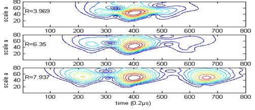
84 D= kHz kHz Time (µs) 125kHz Time (µs) 125kHz kHz kHz Time (µs) Time (µs) 125kHz kHz Time (µs) 125kHz Time (µs) 125kHz kHz kHz Time (µs) Time (µs) Figure 5-4: Time series and wavelet transform of records of impact on the composite plate for three diameters of steel ball at four positions along 0, where D is the diameter of the impact ball in mm. 76

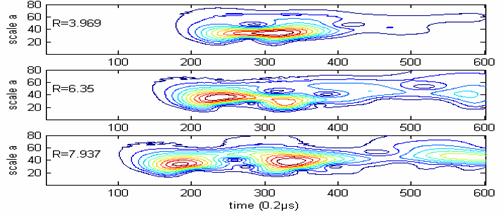
85 125kHz kHz kHz Time (µs) Time (µs) 125kHz kHz kHz Time (µs) Time (µs) 125kHz kHz kHz Time (µs) Time (µs) 125kHz kHz kHz Time (µs) Time (µs) Figure 5-5: Time series and wavelet transform of records of impact on the steel block for three diameters of steel at four positions, where D is the diameter of the impact ball in mm. 77

86 Figure 5-6 summarises the relationship between the time difference between the first two peaks and ball diameter and source-sensor distance, where the time difference turns out to be proportional to ball diameter with a high degree of confidence, R 2 >0.9 for impact on the composite plate and R 2 >0.97 for impact on the steel block and the slope for each trendline (source-sensor distance) is close, between 5 and 6 for the composite plate and 3.4 and 3.6 for the steel block. This means that source-sensor distance has no significant effect on the relationship between the time difference and ball diameter. Accordingly, all of the data are merged in Figure 5-7 to obtain a general relationship between the time difference of the first two peaks and ball diameter which causes a slight drop in the goodness-of-fit. Figure 5-7 also shows the effect of target type on the time difference, where the steel block is more elastic than the composite plate, thus has shorter time difference. Figure 5-6 suggests that changes in the time difference resulting from changes of source-sensor distance are irregular. For example, a bigger time difference appears when the source-sensor distance is 3.5cm than 8.5cm for the composite plate and 5cm for the steel block. Figure 5-8 clarifies this observation, where dark blue, pink and yellow represent the small, middle and big balls, respectively. The average time differences for the three size balls are 23.76, and 44.55µs for the composite plate and 13.45, and 27.27µs for the steel block, and the times randomly distribute within the error bands, ±15%, ±10% and ±15% of means for the composite plate and ±10%, ±5% and ±5% for the steel block. time vs ball diameter vs distance time vs diameter vs distance the time difference (µs) 55 y = x R 2 = y = x 50 R 2 = y = x R 2 = y = x R 2 = the time difference (µs) y = x R 2 = y = x R 2 = y = x R 2 = y = x 15 R 2 = ball diameter (mm) ball diameter (mm) (a) (b) Figure 5-6: The effect of ball diameter and source-sensor distance on the time difference between the first two peaks of the Gabor Wavelet Transform, where dark blue, pink, yellow and cyan represent 4 source-sensor distances, 3.5cm, 5cm, 8.5cm and 10cm for impact on the composite plate and 1.5cm, 3cm, 5cm and 7.5cm for impact on the steel block respectively. (a) Impact on the composite plate; (b) Impact on the steel block. 78

87 time vs. ball diameter time vs. ball diameter the time difference (µs) y = x R 2 = ball diameter (mm) the time difference (µs) y = x R 2 = ball diameter (mm) (a) (b) Figure 5-7: The best fit for the time difference between the first two peaks against ball diameter. (a) Impact on the composite plate; (b) Impact on the steel block. time vs distance drop height = 40mm, angle = 0 degree time vs distance drop height = 40mm 30 the time difference (µs) y = (±10%) y = (mean) y = (±10%) y = (±15%) y = (mean) D=7.937mm y = (±15%) D=6.35 mm 25 y = (±15%) y = (mean) 20 y = (±15%) D=3.969mm the time difference (µs) y = (±5%) y = (mean) y = (±5%) y = (±5%) y = (mean) y = (±5%) D=7.937mm D=6.35 mm 16 y = (±10%) 14 y = (mean) 12 y = (±10%) D=3.969mm source-sensor distance (mm) source-sensor distance (mm) (a) (b) Figure 5-8: The effect of source-sensor distance on the time difference between the first two peaks of the Gabor Wavelet Transform, where dark blue, pink and yellow represent the small, middle and big balls, respectively. (a) Impact on the composite plate; (b) Impact on the steel block. The effect of drop height on the time difference of the first two peaks on its contour plot is summarised in Figure 5-9 (Set-up-2 in Tables 3-3 and 3-4). At each drop height, the 79

88 time difference is still proportional to ball diameter with a high degree of confidence (R 2 >0.9) and the slopes for the different drop heights are still close to each other varying from 4 to 6 for the composite plate and 3.0 to 3.5 for the steel block. The effect of drop height is quite clear for impact on the steel block, where the time difference increases as drop height decreases, but the effect is less clear for impact on the composite plate. In the latter case, although the time difference increases significantly for a drop height of 5cm, there is almost no difference between drop heights of 19cm, 14cm and 10cm. time vs.ball diameter vs.drop height time vs. ball diameter vs. drop height the time difference (µs) 55 y = x y = x 50 R 2 = R 2 = y = x 40 R 2 = y = x 20 R 2 = ball diameter(mm) the time difference (µs) y = x R 2 = y = x R 2 = y = x R 2 = y = x R 2 = ball diameter (mm) (a) (b) Figure 5-9: The effect of drop height on the time difference between the first two peaks in its contour plot, where dark blue, pink, yellow and cyan represent the drop height is 50mm, 100mm, 140mm and 190mm for the composite plate and 40mm, 50mm, 100mm and 140mm for the steel block. (a) Impact on the composite plate; (b) Impact on the steel block. Figure 5-10 shows raw AE waves for a steel ball with diameter of 7.9mm was dropped from a height of 4cm onto the centre of the composite plate and a sensor was placed 5cm away from the impact source along a line at angles 0, 20, 40, 60, 80 and 90 on the surface of the plate (Set-up 3 in Table 3-4). Each wave consists of many pulses with different magnitude, phase and duration. Figure 5-11 shows the effect of angle of the composite plate on the time difference between the first two peaks, and no clear relationship is evident between the time difference and angle. The time difference is randomly distributed within ±5% error bands of mean, i.e. from µs to µs. 80

89 (a) (d) (b) (e) Time (µs) (c) Time (µs) (f) Figure 5-10: Time series of records of impact on the composite plate along different angles, where the dropped ball diameter was 6.35mm. (a) 0º; (b) 20º; (c) 40º; (d) 60º; (e) 80º; (f) 90º. time vs angle drop height = 40mm, distance = 50mm the time difference (µs) 46 y = (±5%) 42 y = (mean) 38 y = (±5%) angle (degree) Figure 5-11: The effect of angle of the composite plate on the time difference between the first two peaks. 81

90 The effect of the composite plate on the time difference between the first two peaks is shown in Figures 5-12 and 5-13, where the impact signals were collected by a sensor placed on the centre of the bottom surface of the composite plate (Set-up-4 in Table 3-4). Figure 5-12 shows typical impact signals and their wavelet transforms, where 3 sizes of steel balls were used to simulate impact sources. Figure 5-13 reveals that the time difference is still proportional to ball diameter and its slope 6.0 is close to that in Figure 5-7 (5.2) where the impact signals were collected by a sensor placed on the surface of the composite plate. That means that the composite plate has an insignificant effect on the time difference between the first two peaks. D=3.969 D= kHz 125kHz Time (µs) Time (µs) D= kHz Time (µs) Figure 5-12: Typical impact signals collected by a sensor placed on the centre of the bottom surface of the composite plate. D is the diameters of impact ball and its unit is mm. 82

91 time vs. ball diameter 55 the time difference (µs) y = 5.969x R 2 = ball diameter (mm) Figure 5-13: The effect of the composite plate. In summary, the time difference between the first two peaks is proportional to ball diameter, sometimes decreases with increasing drop height, and the effects of sourcesensor distance, angle and the composite plate are insignificant. 5.3 Comparison with theoretical contact time According to Hertz s theory, the contact time of dynamic impact between a hard (i.e. elastic) sphere and a hard, flat surface with no flexure is [109]: t f rρ = /10 h E 2 / 5 2 / 5 (5-1) where r and ρ are the radius and density of the sphere, h is the drop height, and the combined Young s modulus E * is given by: 1 E * υ1 1 υ2 = + (5-2) E E 1 2 where E 1, E 2, υ 1 and υ 2 are Young's modulus and Poisson's ratio of the sphere and plate respectively. Equation 5-1 indicates that contact time t f is proportional to ball radius r, but inversely proportional to 10 h. Therefore, the relationships between the time difference between the first two peaks and ball diameter and drop height in Figure 5-7 and Figure 5-9 agree well with Hertz's theory, which suggests that the time between the first two peaks is indeed related to contact time. 83

92 All of the time differences between the first two peaks from impact tests and the corresponding theoretical contact times estimated by Hertz s theory are plotted in Figure 5-14, where the time difference data in Figure 5-14(a) was collected by a sensor placed on the surface of the composite plate, while in Figure 5-14(c) the sensor was placed on the bottom surface of the composite plate purposely to investigate the effect of the composite plate. Figure 5-14 shows generally that the theoretical contact time is proportional to the time difference between the first two peaks with a high degree confidence (R 2 >0.9), and thus the time difference between the first two peaks well represents the theoretical contact time. The time difference between the first two peaks in its contour plot of wavelet transform is hereafter abbreviated to estimated contact time to distinguish it from the theoretical contact time. experiments vs. theory experiments vs. theory theoretical contact time (µs) 50 y = x 45 R 2 = theoretical contact time (µs) y = x R 2 = the time difference (µs) the time difference (µs) (a) (b) experiments vs. theory 45 theoretical contact time (µs) y = x R 2 = the time difference (µs) (c) Figure 5-14: The time difference between the first two peaks vs. the theoretical contact time. (a) Impact on the composite plate; (b) Impact on the steel block; (c) The effect of the composite plate. 84

93 5.4 Discussion Identification of impact wave modes According to Lamb s wave theory flexural modes are stimulated by out-of-plane impulses, and so the signals in Figure 5-12 can be attributed to flexural waves. The flexural waves may involve some in-plane motion (extensional waves) due to the Poisson effect, which can be seen in Figure 5-2, in the initial small high frequency waves visible at a drop height of 50mm, but barely visible at 40mm. Generally speaking, the AE waves generated by dropped objects contain a larger flexural wave and a smaller extensional wave Application of the estimated contact time a) Estimation of Young s Modulus The Young s Modulus of the impacted target can be estimated from the estimated contact time assuming the Hertz theory to be valid. From Equation 5-1, E * can be expressed as follows, E = (( r t f 3.76ρ ) 1/10 h 2 / 5 ) 5 / 2, i.e. E h 1/10 2 / 5 5 / 2 f -5 / 2 = (3.76ρ ) ( ) (5-3) r t That means that E is proportional to h ( t r 1/10 f ) -5 / 2. Since E is constant for impact between two given materials, so is the value of h ( 1/10 r t f ) -5 / 2. 6 t f ( y 10 ) 2 y Since ( s / m) = ( s / m) = ( s / m) 3 r ( x 10 / 2) 1000 x the best fit curve in Figure 5-7, we can write:, where y / x is the rate of slope of y y E = ( ) ( h ) = (1880 )( h ) x x 2 / 5 5 / 2 1/10-5 / 2 5/2 1/10-5 / 2 ρ ρ (5-4) 85

94 Solving Equation (5-2) for the (variable) modulus of the target material: E 2 = 1 E 1 υ υ E (5-5) The estimated Young s modulus of the impacted targets is listed in the Table 5-1. The value of h ( 1/10 r t f ) -5 / 2 remains constant within the error band (±11.6% for the composite and ±4.8% for the steel block), which verifies again that the time difference between the first two peaks in the contour of the wavelet transform is indeed related to the contact time of impact. The error for the composite plate is bigger than that for the steel block, probably because the composite is viscoelastic and incurs a bigger error when estimates use Hertz's theory. Composite plate Impacted target Steel block (h 1/10 y / x) -5/ Mean Std Max Error ( )/ = 11.6% ( )/ = 4.8% Estimated E * (GPa) from Equation (5-4) Estimated E 2 (GPa) from Equation (5-5) Mean Std Error relative to empirical values (60-36)/60=40% ( )/210=6.2% Table 5-1: Estimated Young s modulus of impact targets. 86

95 In Figure 5-14(b), the best fit for the impact on the steel block is close to y = x, which means the estimated contact time is most likely the contact time of impact. However, the estimated contact time is slightly longer than the theoretical contact time for the composite plate where y = x in Figure 5-14(a) and y = x in Figure 5-14(c). This is probably again due to the fact that the steel block and balls will behave in a linear elastic fashion over a wider rage of strains than the composite, despite the fact that it is generally accepted that elastic behaviour can be assumed when the volume fraction of fibres is greater than that of matrix [109] and this condition is met for the composite used here (58% fibres and 42% matrix). Stronge [109] suggests that a linear Maxwell model is more accurate than assuming linear elastic behavior in Hertz s theory for a composite. He has compared the two and verified that the former gives a slightly longer contact time. This adequately explains why the theoretical contact time estimated by Hertz s theory is shorter than the estimated contact time in Figure 5-14(a) and Figure 5-14(c). b) Determination of impact wave speeds The distinct characteristic of an AE impact wave is that it consists of many pulses with different magnitude, phase and duration, while the number of pulses in each wave varies, and, moveover, the magnitude, phase and duration of waves distort due to dispersion, attenuation, and reflection during propagation, which makes it difficult to find the counterparts of arrival times [77]. Figure 5-15 shows waves propagating along 0 and 45 degree lines, respectively, with the distances between sensors being 10cm along the 0 degree line and 14.14cm along the 45 degree line. There are at least two ways to determine the arrival times marked with red and yellow lines/circles, depending upon whether the phase of the pulses is considered or not. The confusion can be solved if the estimated contact time is introduced, however. As discussed above, the estimated contact time remains constant with a given dropped ball and drop height, so it is easily recognized, and thus the associated peaks can be located for arrival time determination. The peaks marked with red circles in Figure 5-15(a) and yellow in Figure 5-15(b) are selected as arrival times, based on the estimated contact time, which suggests that the phase of pulses has no effect on arrival time determination. For example, the wave speeds obtained in this way are around 1144m/s and 1107m/s at the angles of 0 and 45 degrees respectively. This seems to suggest that the impact wave speeds are angle- 87

96 independent, which conforms with the measured result for the flexural wave in Chapter 4. S4 S3 S2 S1 (a) S4 S3 S2 S1 (b) Figure 5-15: Time series of records of impact wave propagation along 0º and 45º. (a) 0º; (b) 45º. 88

97 Chapter 6 Destructive tests In composites, AE signals can be generated by various damage sources, the main ones being fibre breakage, matrix cracking, fibre-matrix de-bonding and delamination. As yet, little consensus has been claimed in the literature in discriminating between these damage modes in composites. In this chapter, the results from the destructive tests have been analysed with a view to assessing the characteristics of the AE generated in each of the three modes of overloading: tension, bending and tearing. The load-ae-time characteristics are first examined for where the main concentrations of AE events occur during the tests. Next, some samples of AE during the tests are analysed in the time-frequency domain to assess whether the findings are consistent with the wave mode analysis techniques that have been suggested by some authors for discriminating damage modes. 6.1 Strength of composites and structure of specimens The strength of a unidirectional continuous fibre reinforced composite when loaded along the fibre direction can be considered as a case of parallel loading, as shown in Figure 6-1, where the stress is shared between the fibres and the matrix in proportion to their volume fractions and the strain in the composite is the same as in each of the components. At relatively high volume fractions, V f, of fibres (usually above about 0.1), the strength of a * composite in the fibre direction, σ 1, depends upon whether the fibres fail at a lower strain than the matrix or vice versa [114, 115, 116]: 89

98 ( V ) σ + V σ σ 1 = 1 f m f f (for brittle fibres) (6-1) σ 1 = V f σ f (for brittle matrix) (6-2) * where σ f is the fibre failure stress and σ m is the matrix stress, when the strain equals the fibre failure strain, ε. * f Fibres σ 1 σ 1 Matrix Figure 6-1: The parallel loading model for composite strength. For the brittle matrix case, considerable cracking occurs in the matrix prior to failure of the composite (Figure 6-2) as the fibres continue to be able to take further strain beyond the matrix failure strain, ε. In the case of the brittle fibre model, failure of the fibres * m sheds all of the load onto the matrix, which is then unable to carry the load as its failure stress is exceeded. As mentioned in Chapter 3, the material used was carbon-fibre reinforced epoxy laminate, 5mm thick, comprising 17 woven plies. The plies were in a 4 4 twill weave, meaning that each strand passes over four of the perpendicular strands before passing under four strands. The fibres are arranged in strands of 3000, and are made of Thornel T300 PAN precursor fibre. This type of fibre has a diameter of 6.93μm, a tensile strength of 3240MPa, and a tensile modulus of 231GPa [117], giving a failure strain linear elastic behavior up to fracture) of 1.4%. * ε f (assuming 90

99 Fibre fails σ 1 * Matrix fails V f σ f * Stress Composite stress-strain curve V f σ f (fibre component) (1-V f ) σ m (matrix component) ε m * Strain (a) ε f * σ 1 * Fibre fails, and matrix unable to withstand the stress (1-V f ) σ m +V f σ f * Composite stress-strain Stress V f σ f (fibre component) (1-V f ) σ m (matrix component) ε f *, ε m Strain ε m * (b) Figure 6-2: Brittle matrix model and brittle fibre model. (a) Brittle matrix model; (b) Brittle fibre model. 91

100 It is not known precisely which epoxy material was used, but it is likely to be either tetraglycidyl methylene dianiline (TGMDA) or diglycidyl ether of bisphenol (DGEBA) each cured with diaminodiphenyl sulphone (DDS), the key properties of which are shown in Table 6-1 [118]. Epoxy type Tensile strength (MPa) Tensile modulus (GPa) Elongation (%) TGMDA/DDS DGEBA/DDS Table 6-1: The key properties of epoxy used. Irrespective of the type of epoxy, it is therefore clear that the composite conforms to a brittle fibre model so that the fibres and matrix will fail at the same overall strain (1.4%). According to the brittle fibre model, for uniaxial fibres parallel to the tensile direction, the failure stress will be [117]: * ' * * * σ1 = (1 Vf ) σm + Vfσ f = 0.42Emε f σ f [ ] MPa (6-3) giving a tensile strength of about 2000MPa for a uniaxial composite. Because the uniaxial composite fails at a single value of strain, it might be expected that matrix cracking will account for only about 1% of the strain energy at failure. Given that only half of the fibres are aligned in the tensile direction, the contribution to the laminate strength will be diluted and, as a first approximation, the overall strength can be taken as the average between the uniaxially-aligned value calculated above and that transverse to the fibre direction [117]: E σ2 = [1 ( V V )(1 )] σ [48 96] MPa (6-4) * m * f f E m f which is essentially equal to the matrix strength. Thus, the overall strength of the composite should be approximately 1000MPa, and the strain energy associated with fibre-matrix de-bonding is only about 10% of the total, 92

101 probably released before failure of the composite. Figure 6-3 shows the structure of the composite at various magnifications. The macro-photograph shows the tows (strands) to be around 1.5mm wide and the low-magnification micrograph shows them to be about 0.2mm thick, in reasonable accord with the ply thickness (laminate thickness divided by number of plies) of 0.3mm, the difference being accountable by the fact that the plies are not flat. The high-magnification micrograph shows the fibres to be around 5μm in diameter, again in reasonable accord with the published value of 7μm, given that these are random longitudinal sections not guaranteed to go through the axis of the fibre. 50 μm 10 mm 1 mm Figure 6-3: The structure of the composite at various magnifications Figures 6-4 show various views of the tensile and bending failures confirming the de-bonding of the matrix from the transverse fibres and the simultaneous failures of matrix and fibres in the longitudinal direction. 93

102 Figure 6-4: Various views of the tensile and bending failures 6.2 Modal AE analysis method for discrimination of damage modes According to Lamb s wave theory, extensional modes and flexural modes are caused by motions in-plane and out-of-plane respectively. In cross-ply composites subject to axial tension, it might therefore be expected that fibre/matrix de-bonding and fibre breakage will generate AE waves which contain a predominantly flexural and extensional modes respectively, while matrix cracking will generate both extensional and flexural modes. Fibre/matrix de-bonding may involve some in-plane motion due to the Poisson effect, but the in-plane motion will be smaller than the out-of-plane and thus will produce a smaller amplitude extensional mode [53]. In cross-ply composites subject to bending, fibre breakage will generate a predominantly flexural mode, because breakage and hence wave generation will be confined to the tensile side and thus the motion will be asymmetric about the mid-plane [48]. In Chapter 4.1.2, the wave generated by a pencil lead break on the edge of the specimen was identified as an extensional wave with a characteristic frequency at 167kHz, while the wave generated by a pencil lead break on the surface was identified as flexural with a characteristic frequency of 125kHz; both waves had a component at around 330kHz, 94

103 so this could not be used for identification purposes. Thus, the proportions of the energy of the signal of a given event in the two bands around 125kHz and 167kHz should give an idea of whether the event is predominantly giving rise to an extensional wave (fibre breakage) or a flexural wave (fibre/matrix de-bonding). Events which do not fit neatly into either category could be associated with multiple sources and/or matrix cracking. 6.3 Results from mechanical tests Figures 6-5 to 6-7 give a general view of the AE activity during the whole process of each mechanical test, where the signals were collected by the trigger sensor. As can be seen, AE energy is released throughout the tests, but most intensely in the final stages, most probably by fracture. How much energy and how rapidly it is released could be related to the different failure mechanisms, and the proportions of these could change during the test. To give an overview, conventional AE energy analysis was applied to the curves, with AE energy rate and AE cumulative energy being calculated using the following equations: e( j) = A 2 j A 2 j t (for energy rate) (6-5) i i 2 2 A j 1 + A j E( i) = e( j) = t (for cumulative energy) (6-6) j= 1 j= 1 2 where A = 0 0, i 1 and j 1, A j is the amplitude of the AE signal at time t j and 1 t = is the time difference between t 6 j-1 and t j, kept constant. This time difference 5 10 was chosen by inspection of the early stages of the record so as to represent about twice the event length minimising the danger of capturing more than one non-overlapping event. The units of both energy rate and cumulative energy are volt 2 second. Cumulative AE energy, AE energy rate and stress/load against time are shown in Figures 95

104 6-5 to 6-7 where Figure 6-5 represents the three-point bending test on an unnotched sample, Figure 6-6 the tensile test on an unnotched sample and Figure 6-7 the tearing test on a notched sample. In the unnotched tensile test, the stress increases in an approximately linear fashion and there is an abrupt drop to zero at the critical stress, and corresponding strain, taken to be the fibre failure strain, is 1% roughly. In the bending test, there is a similarly abrupt drop to zero from a linearly increasing stress, defined as the maximum tensile stress on the outer fibres of the bend. Equations 6-1 to 6-3 calculate failure strainε f, stressσ f and Young s modulus E respectively, where L, b, d are the support span, width and depth of the tested sample, and D max, F max are the maximum central deflection and the maximum load in the bending test [119]: ε f 6Dmaxd = = = % (6-7) L 210 σ f 3FmaxL = = = MPa (6-8) 2 2 2bd f E = σ = = 62.9 GPa (6-9) 2 ε f leading to an estimate of the fibre failure strain of about 1%. In the case of the notched tearing test seen in Figure 6-7, the stress (and, hence, load) does not fall to zero immediately due to the fact that the compliance increases rapidly on first failure and the tear does not completely traverse the specimen. The total amount of AE energy recorded during each of the tests was around the same order of magnitude, although the bending test produced generally about 1.5 times as much AE as the tensile test and about twice as much as the tearing test. As might be expected from the concentrated stress, the steepest jump in energy at failure was in the tearing test, with more gradual evolutions in the bending and tensile tests, with the tensile 96

105 test producing AE almost from the beginning. Bending Test Cumulative Energy / Energy Rate (v 2 s) 2.00E E E E E E E E E E E Time(s) σ(mpa) Energy Rate Cumulative Energy σ (a) Bending Test Energy Rate (v 2 s) 4.40E E E E E E E E E E E E+00 failure point Time(s) Energy Rate (b) Figure 6-5: Stress, AE cumulative energy and AE energy rate in the bending test. (a) Stress, AE cumulative energy and AE energy rate and; (b) Magnified AE energy rate only. 97

106 Tensile Test Cumulative Energy / Energy Rate (v 2 s) 1.00E E E E E E E E E E E σ(mpa) Energy Rate Cumulative Energy σ Time(s) (a) Tensile Test Energy Rate (v 2 s) 2.40E E E-05 failure point 1.20E E E E Time(s) Energy Rate (b) Figure 6-6: Stress, AE cumulative energy and AE energy rate in the tensile testing. (a) Stress, AE cumulative energy and AE energy rate; (b) Magnified AE energy rate only 98

107 Tearing test Cumulative Energy / Energy Rate (v 2 s) 8.00E E E E E E E E E Time(s) Force(N) Energy Rate Cumulative Energy Force (a) Tearing test Energy Rate (v 2 s) 3.50E E E E E E E E+00 failure point Time(s) Energy Rate (b) Figure 6-7: Load, AE cumulative energy and AE energy rate in the tearing test. (a) Load, AE cumulative energy and AE energy rate; (b) Magnified AE energy rate only. 99

108 6.4 Identification of source modes In order to identify the sources, it was first necessary to separate out the individual AE event signatures from the tests, insofar as this was possible. Each test record consisted of seconds of data, much of it containing no significant AE. This record was de-noised by setting up a threshold to the acquisition system before the tests to prevent environmental noise and smoothed using 30-point moving averages. Events were located in the record by the threshold crossing technique, where the threshold of 0.01V was considered small enough to collect all but the insignificant events. The events were typically of duration to second and each was transformed into the frequency domain using an FFT algorithm. Figures 6-8 to 6-10 show the frequency distributions of all AE events generated during the three tests. Three dominant frequency bands around 125kHz, 167kHz and 333kHz appear, as with the AE signals generated in the pencil lead break tests reported in Chapter 4.1. Generally speaking, the high frequency band (333kHz) is amplified disproportionately due to its nearness to the resonant frequency of the sensors. Events Frequency (Hz) Figure 6-8: Frequency distribution of AE events in the bending test 100

109 Events Frequency (Hz) Figure 6-9: Frequency distribution of AE events in the tensile test 101

110 Frequency (Hz) Figure 6-10: Frequency distribution of AE events in the tearing test 102

111 Following the hypothesis presented in Chapter 6.2, all the events generated in the tensile tests and tearing tests were categorised into one of three groups: fibre breakage related, fibre/matrix de-bonding related and matrix cracking related, according to the rules shown in Table 6-2. An event was classified as being in the 167kHz domain if the maximum magnitude at 167kHz is not less than 0.4 times of that at 333kHz in its contour plot and it contains a small component at 125kHz, and hence was categorised as fibre breakage related. Similarly an event was classified as being in the 125kHz domain if the maximum magnitude at 125kHz is not less than 0.4 times of that at 333kHz in its contour plot and it contains a small component at 167kHz, and hence was categorised as fibre/matrix de-bonding related. The other events, i.e. those with weak 125kHz and 167kHz components or with close maximum magnitudes at 125kHz and 167kHz were assigned to the matrix cracking related group, although it is acknowledged that these may contain mixed events. The factor of 0.4 for the frequency component of 333kHz was selected somewhat arbitrarily, although it gives a scaling relative to the overall event size, which would not be possible by simply using the ratio of 125kHz:167kHz. For the bending test, since events will mostly be generated at the tensile side, the motion will be asymmetric about the midplane [48] irrespective of the generating event, leading to most waves generated being flexural. Therefore all events generated in bending tests were categorised into two groups: fibre breakage related and other damage modes, according to the rules shown in Table

112 Group Fibre breakage Fibre/matrix de-bonding Matrix cracking Modal 167kHz magnitude is not less 125kHz magnitude is not less the rest AE Features than 0.4 times of that of 333kHz than 0.4 times of that of 333kHz 125kHz absent or much smaller 167kHz absent or much smaller Table 6-2: Categorisation rules for events generated in the tensile and the tearing tests Group Fibre breakage Other damage modes Modal AE Features 125kHz magnitude is not less than 0.4 times the rest of that of 333kHz 167kHz absent or much smaller Table 6-3: Categorisation rules for events generated in the bending test As an example of classification, Figure 6-11 shows a typical event signature frequently appearing in the tearing test. It is classified as 167kHz (scale=30) domain as the amplitude is more than 0.4 times of that of 333kHz (scale=15), with 125kHz (scale=40) being absent. This type of event signature was repeated around 190 times during the test. The small specimen used for the tearing test contains 8 fibre strands running in the tensile direction, where each strand consists 3000 of single fibres. It is therefore not likely that the events correspond to individual fibre breakages, but rather to groups of fibres breaking, perhaps whole strands. 104

113 Frequency f (khz) kHz 333kHz Figure 6-11: Typical fibre breakage wave signal in the tearing test, where x/ is the time in seconds, and y is scale (upper figure) or amplitude (lower figure). Figure 6-12 is more representative of the events occurring at the fracture stress in the bending test. They are all the flexural waves with 125kHz (scale = 40) domain with its amplitude more than 0.4 times of that of 333kHz (scale = 15), and with 167kHz (scale = 30) absent. Hence fibre breakage events must be those in the 125kHz domain and its amplitude is not less than 0.4 times of that of 333kHz, with 167kHz absent or much smaller, which conforms with the theory outline in Section Frequency f (khz) kHz 333kHz 105

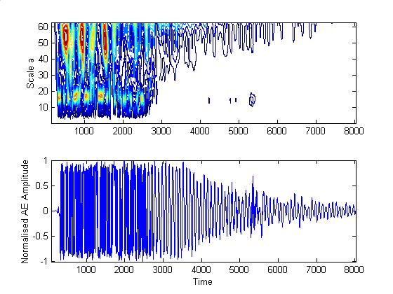
114 Frequency f (khz) kHz 333kHz Frequency f (khz) kHz 333kHz Frequency f (khz) kHz 333kHz 106