Manifold Learning: From Linear to nonlinear. Presenter: Wei-Lun (Harry) Chao Date: April 26 and May 3, 2012 At: AMMAI 2012

Transcription

1 Manifold Learning: From Linear to nonlinear Presenter: Wei-Lun (Harry) Chao Date: April 26 and May 3, 2012 At: AMMAI

2 Preview Goal: Dimensionality Classification reduction and clustering Main idea: What information and properties to preserve or enhance? 2

3 Outline otation and fundamental of linear algebra PCA and LDA opology, manifold, and embedding MDS ISOMAP LLE Laplacian eigenmap Graph embedding and supervised, semi-supervised extensions Other manifold learning algorithms Manifold ranking Other cases 3

4 Reference [1] J. A. Lee et al., onlinear Dimensionality reduction, 2007 [2] R. O. Duda et al., Pattern Classification, 2001 [3] P.. Belhumeur et al., Eigenfaces vs. Fisherfaces, 1997 [4] J. B. enenbaum et al., A global geometric framework for nonlinear dimensionality reduction, 2000 [5] S.. Roweis et al., onlinear dimensionality reduction by locally linear embedding, 2000 [6] L. K. Saul et al., hink globally, fit locally, 2003 [7] M. Belkin et al., Laplacian eigenmaps for dimensionality reduction and data representation, 2003 [8]. F. Cootes et al., Active appearance models,

5 otation Data set: ( n) d high-d: X { x R } n 1 ( ) low-d: { y n p } n Y R 1 Matrix: Vector: A a Matrix form of data set: (1) (2) ( m) nm [ a, a,..., a ] [ aij ] 1 in,1 jm [ a, a,..., a ] ( i) ( i) ( i) ( i) d1 1 2 d (1) (2) ( ) (1) (2) ( ) X d x, x,..., x x x... x 5

6 Fundamental of Linear Algebra SVD (singular value decomposition): X d (1) v (2) 0 (1) (2) ( ) d Ud d d V... v u u u dd ( ) dd 0d v, where (1) u (2) (1) (2) ( d ) U U u u u... u Idd, V V I ( d) dd u dd U U I UU, V V I VV U U, V V 1 1 6

7 Fundamental of Linear Algebra SVD (singular value decomposition): d = * 0 * d = * 0 * 7

8 Fundamental of Linear Algebra A EVD (Eigenvector decomposition) u u (1) (2) ( ) (1) (2) ( ) AU U A u u u u u u A UU A U U Caution: Eigenvalues are not always orthogonal! Caution: ot all the matrices have EVDs. 8

9 Fundamental of Linear Algebra Determinant: race: A n n1 tr( A ) diag( A) a ii n n1 n1 tr( A B ) tr( B A ) d d d d Rank: rank( A) rank( UV ) # nonzero diagonal elements of # independent columns of A # nonzero eigenvalues (square A) rank( AB) min( rank( A), rank( B)) rank( AB) rank( A) rank( B) 9

10 Fundamental of Linear Algebra SVD vs. EVD (symmetric positive semi-definite) A XX UV ( UV ) U( V V ) U U ( ) U AU U( ) U U U ( ) U U Hermitian matrix: A A conj( A) A is real A A H AU A UV ( UV ) VU A U V A U U AU U U AU Hermitian matrices have orthonormal eigenvectors. 10

11 Dimensionality reduction Operation: ( n) d high-d: X { x R } ( n) n 1 p low-d: Y { y R } n 1 ( p d) Reason: Compression Knowledge discovery or feature extraction Irrelevant and noise feature removal Visualization Curse of dimensionality 11

12 Dimensionality reduction Methods: Feature Feature transform: selection: Criterion: Preserving hese d p : xr yr, p d some properties or structures of the high-d feature space into the low-d feature space. properties are measured from data. f linear form: y ( ) x Qp d y [ x, x,..., x ] s s(1) s(2) s( p) deotes selected indices 12

13 Dimensionality reduction Model: f d p : xr yr, p d Linear projection: y ( Q ) p d x Direct re-embedding: X { x R } Y { y R } ( n) d ( n) p n1 n1 Learning a mapping function: 13

14 Principal Component Analysis (PCA) [1] J. A. Lee et al., onlinear Dimensionality reduction, 2007 [2] R. O. Duda et al., Pattern Classification,

15 Principal component analysis (PCA) PCA: ( Q ) Q I d p d p p p (1) q (2) ( Qd p) q y x = x ( p ) q pd ^ (1) (2) ( p) x x Qd py = q q... q y p 15

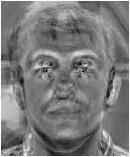
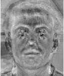
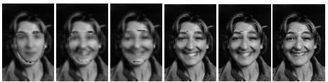
16 Principal component analysis (PCA) Surprising usage: face recognition and encoding = = 16

17 Principal component analysis (PCA) PCA is basic yet important and useful: Easy Lots to train and use of additional functionalities: noise reduction, ellipse fitting, Also named Karhunen-Loeve transform (KL transform) Criteria: Maximum Minimum variance (with decorrelation) reconstruction error 17

18 Principal component analysis (PCA) Maximum variance (with decorrelation) Minimum reconstruction error 18

19 Principal component analysis (PCA) (raining) data set: Preprocessing: centering (mean can be added back) Model: ( n) d high-d: X { x R } n 1 ( n) x x Xe n1 1 ( n) ( n) X X xe X ( I ee ), or say x x x p y Q x, where y R and Q is d p Q Q I p p (orthonormal) ^ x Qy = QQ x 19 n1

20 Maximum variance (with decorrelation) he low-d feature vectors should be decorrelated Covariance variance: Covariance matrix: C xx 1 cov( x, x ) E ( x x )( x x ) ( x x )( x x ) ( n) ( n) n 1 (1) x cov( x1, x 1) cov( x1, xd ) (2) 1 (1) (2) ( )... x x x x cov( xd, x1 ) cov( xd, xd ) ( ) x 1 ( )( n1 ( n) ( n x x x ) x) X( I ee )( I ee ) X 1 1 (1) (1) ( ) ( ) x x... x x 20

21 Maximum variance (with decorrelation) Covariance matrix 1 cov( x, x ) E ( x x )( x x ) ( x x )( x x ) ( n) ( n) n 1 21

22 Maximum variance (with decorrelation) Decorrelation: 1 ( n) 1 ( n) y y Q x Q x n1 n1 0 1 ( n) ( n) 1 ( n) ( n) 1 ( n) ( n) Cyy ( y y)( y y) ( Q x )( Q x ) Q ( x )( x ) Q n1 n1 n1 Q C Q diagonal matrix xx 22

23 Maximum variance (with decorrelation) Maximum variance Q 1 1 arg max arg max y y Q x Q QI 2 * ( n) ( n) 2 arg max Q QI Q QI n1 n1 1 1 arg max ( ) ( ) arg max Q x Q x QQ x Q QI ( n) ( n) ( n) ( n) Q QI n1 n1 1 1 ( n) ( n) ( n) ( n) tr{ x QQ x } arg max { } tr Q x x Q Q QI n1 n1 (1 x 1) (p x p) x 1 ( n) ( n) arg max tr{ Q [ ] } arg max { } x x Q tr Q C xxq Q QI Q QI n1 23

24 Maximum variance (with decorrelation) Optimization problem: C yy Q arg max tr{ Q C Q} subject to diagonal C and QQ I * d p xx yy Q Solution: Q u Q CxxQ * (1) (2) ( p) C C C () i C xx [ u, u,..., u ], xx xx xx is the ith largest eigenvector of C R dd Cxx XX UV V U U ( ) U UU * * Q Q I p p xx 24

25 Maximum variance (with decorrelation) Proof: Assume q is d 1, tr{ q C q} q C q xx xx * q arg max q C xxq q q1 E q q Cxxq ( qq1) arg max (, ) arg max q, q, Lagrange multiplier ake partial derivative 0 E ( Cxx Cxx ) q 2q 0 C q E qq 1 0 xx q q eigenvector q * is the largest eigenvector of Cxx * * * * q Cxxq q UU q = 1 25

26 Maximum variance (with decorrelation) (1) (1) q (1) (1) (1) Assume Q q q is d 2, tr{ Q CxxQ} tr{ Cxx } C q q q xxq q Cxxq q * q q C xxq q q1 (1) qq arg max the second largest eigenvector of q C q q UU q = * * * * xx 2 C xx r r ( r ) ( i ) ( i ) Assume Q Qd r qis d ( r 1), tr{ Q CxxQ} q Cxxq q Cxxq i q Cxxq i1 i1 * q q xxq q q1 (1) ( r ) qq... q th arg max C the ( r 1) largest eigenvector of C q C q q UU q = * * * * xx r1 xx 26

27 Minimum reconstruction error Mean square error is preferred: 1 1 Q arg min min x Qy QQ x x Q QI * ( n) ( n) 2 ( n) ( n) 2 Q QI n1 n1 1 ( n) ( n) arg min (( ) ) (( ) ) Idd QQ x Idd QQ x Q QI n arg min ( ) x x x QQ x x Q Q Q Q x Q QI arg min Q QI ( n) ( n) ( n) ( n) ( n) ( n) n1 n1 n1 1 1 x x x QQ x ( n) ( n) ( n) ( n) n1 n1 1 arg ( n) ( n) max arg max { } x QQ x tr Q C xxq Q QI Q QI n1 27

28 Algorithm (raining) data set: Preprocessing: centering (mean can be added back) x Model: ( n) d high-d: X { x R } n 1 n1 x p y Q x, where y R and Q is d p Q Q ( n) 1 ( n) ( n) X X xe X ( I ee ), or say x x x I Xe p p (orthonormal) ^ x Qy = QQ x 28 n1

29 Algorithm Algorithm 1: (EVD) d 1 1. U C U, where in are in descending order xx i i (1) (2) ( d) I p p (1) (2) ( p) 2. Q UId p u u... u... O u u u ( d p) p Algorithm 2: (SVD) d ii 1 1. X UV, where in are in descending order (1) (2) ( d) I p p (1) (2) ( p) 2. Q UId p u u... u... O u u u ( d p) p 29

30 Illustration What is PCA doing:

31 Summary PCA exploits 2 nd order statistical properties measured in data (simple and not vulnerable to over-fitting) Usually used as a preprocessing step in applications Rank: UC U xx 1 ( n) ( n) 1 (1) (1) 1 ( ) ( ) Cxx x x... n 1 x x x x rank( C ) 1, p 1 in general xx 31

32 Optimization problem Convex or not? * q q C xxq = q Cxxq q q q q1 q arg max arg max, s.t. 1 q C xx q 1 1 (1) Cxx XX U ( ) U semi-postive definite (2) q q 1 quadratic equality constraint q q 1 Convex or not? * q q C xxq = q Cxxq q q q q1 q arg min arg min, s.t (1) Cxx XX U ( ) U semi-postive definite (2) q q 1 quadratic equality constraint q q 1 32

33 Examples Active appearance model: ^ x Qy = QQ x [8] [8] 33

34 Linear Discriminant Analysis (LDA) [2] R. O. Duda et al., Pattern Classification, 2001 [3] P.. Belhumeur et al., Eigenfaces vs. Fisherfaces,

35 Linear discriminant analysis(lda) PCA is unsupervised LDA takes the label information into consideration Achieved low-d features are efficient for discrimination. 35

36 Linear discriminant analysis(lda) (raining) data set: Model: otation: ( n) d high-d: X { x R } n 1 p y Q x, where yr and Q is d p X label l ( n) ( n) i i { x ( x ) i} n1 i # samples in X class mean: 1 1 total mean: i i i x n1 ( n) X x i ( n) x ( n) label L l l l c ( n) ( x ) { 1, 2,..., } between-class scatter: S ( )( ) B i i i i1 within-class scatter: S c c ( n) ( n) W ( x i )( x i ) i1 ( n) x X i 36

37 Linear discriminant analysis(lda) Properties of scatter matrix: S S c ( )( ) inter-class separation B i i i i1 c ( n) ( n) W ( x i )( x i) intra-class tightn s i1 ( n) x X i Scatter matrix in low-d: c between-class: ( Q Q )( Q Q ) Q S Q i1 i i i c ( n) ( n) within-class: ( Q x Q i) Q x Q i) Q SW Q i1 ( n) x X i es B 37

38 Linear discriminant analysis(lda) 38

39 Criterion and algorithm Criterion of LDA: Maximize the ration of Q S Qto Q S Q "in some se nse" Determinant and trace are suitable scalar measures: With Rayleigh quotient: S Q B * W B Q S * BQ tr( Q SBQ) Q arg max or arg max Q Q ( Q S Q tr Q S Q ), S are both symmetric positive semi-definite and S Q S Q W B ( i) ( i) arg max S, i is in descending order Bu isw u Q Q SW Q W W W is nonsigular Q u * (1) (2), u,... u ( p) 39

40 ote and Problem ote: S u S u S S u u ( i) ( i) 1 ( i) ( i) B i W W B i rank( S ) c 1, at most c 1 nonzero B so pc1 Problem: rank( S ) c, and S is d d W W if rank( S ) d, S is singular, Rayleight quotient is useless W W i 40

41 Solution Problem: Solution: S PCA+LDA: c ( n) ( n) W ( x i )( x i) is singular i1 ( n) x X i 1. Perform Q on x, x Q x R ( n) ( n) ( n) c PCA( d( c)) PCA 2. Compute S, if nonsingular, the problem is solved W (( c) ( c)) 3. For new samples, y Q ull-space: Q S Q LDA Q PCA * B * 1. Q arg max find Q to make Q SWQ 0 Q Q SWQ * 2. Extract columns of Q from the null space of x S W 41

42 Example [3] 42

43 opology, Manifold, and Embedding [1] J. A. Lee et al., onlinear Dimensionality reduction,

44 opology Geometrical point of view If he two or more features are latently dependent, their joint distribution does not span the whole feature space. dependence induces some structures (object) in the feature space. gb () ga ( ) ( x, x ) g( s), a s b

45 opology opology: Allowed: ot opology A opology Ex: Deformation, twisting, and stretching allowed: earing object means properties and structures topology object (space) is represented (embedding) as a spatial object in the feature space. abstracts the intrinsic structure, but ignores the details of spatial object. circle and ellipse are topologically homeomorphic 45

46 Manifold Feature space: dimensionality + structure eighborhood: opology space can be characterized by neighborhoods Manifold is a locally Euclidean topological space Euclidean space: ei R B d () i ( x ) ball ( x) { x x } L dis (1) (2) (1) (2) ( x, x ) x x is meaningful L In general, any spatial object that is nearly flat in small scale is a manifold

47 Manifold [5] 3D+non-Euclidean 2D 47

48 Embedding Embedding: Embedding A he is a representation of a topological object (ex. a manifold, graph) in a certain feature space, in such a way the topological properties are preserved. smooth manifold is differentiable and has functional structure to link the features with latent variables. dimensionality of a manifold is the # latent variables A k-manifold can be embedded to any d-dimensional space with d is equal to or larger than (2k+1) 48

49 Manifold learning Manifold learning: Recover the original embedding function from data. Dimensionality reduction with the manifold property: Re-embed a k-manifold in d-dimensional space into a p- dimensional space with d >p g () s 2 Latent variables s f() s g () s 1 p-dimensional space hs () d-dimensional space 49

50 Example g () b 1 g ( a) 1 Re-embedding f : g1( s) g2( s) g ( a) 2 g () b 2 ( x, x, x ) g ( s), a s b ( x, x ) g ( s), a s b Latent variable: a a sb b 50

51 Manifold learning Properties to preserve: Isometric embedding: distance preserving dis (1) (2) (1) (2) ( x, x ) dis( y, y ) Conformal embedding: angle preserving angle (1) (3) (2) (3) (1) (3) (2) (3) ( x x, x x ) angle( y y, y y ) opological embedding: neighbor / local preserving Input space: locally Euclidean Output space: user defined 51

52 Multidimensional Scaling (MDS) [1] J. A. Lee et al., onlinear Dimensionality reduction,

53 Multidimensional Scaling (MDS) Distance preserving: dis ( ) ( ) ( ) ( ) ( x i, x j ) dis( y i, y j ) Scaling refers to construct a configuration of samples in a target metric space from information of interpoint distances ? 9 53

54 Multidimensional Scaling (MDS) MDS: a scaling where the target space is Euclidean Here we mentioned about classical metric MDS Metric MDS indeed preserves pairwise inner product rather than pairwise distance Metric MDS is unsupervised 54

55 Multidimensional Scaling(MDS) (raining) data set: Preprocessing: centering (mean can be added back) Model: ( n) d high-d: X { x R } n 1 x n1 x ( n) 1 ( n) ( n) X X x1 = X ( I ee ) or say x x x d p f : x R y R, p d here is no Q to train n1 55

56 Criterion Inner product (scalar product): s ( i, j) s( x, x ) x x x x X ( i) ( j) ( i) ( j) ( i) ( j) Gram matrix: recording pairwise inner product (1) x (2) (1) (2) ( ) S [ sx ( i, j)] x 1 i, j x x... x X X. ( ) x 1 Gram matrix: S X X, Covariance matrix: C X ( I ee )( I ee ) X Usually, we only know Z, but not X 56

57 Criterion Criterion 1: * ( i) ( j) 2 2 p arg min ( ij y y ) arg min arg min Y Y F Y i1 j1 Y s S Y Y S Y Y 2, where A is the L matrix norm, also called the Frobenius norm F a a A ( a ) tr( A A) tr( F i, j a Criterion 2: (1) (2) 2 1/2 (1) (2) ( ) 1/2 ij a a... a ) ( ) (1) y (2) y (1) (2) ( ) X X S Y Y y y... y ( ) y 57 F

58 Algorithm Rank: (assume >d) rank ( X X ) min(, d ), rank ( Y Y ) min(, p ) Low-rank approximation: d A R with rank( A) r 0, A UV I O * * kk B arg min A B U V ran( B) k F O O kr (1) v (2) (1) (2) ( d ) kk O... v u u u O O dd ( ) v 58

59 Algorithm EVD: (Hermitian matrix) Solution: S X X ( U V ) ( U V ) V ( ) V V V ( ) O Y Y V V V I I V O O p p 1/2 1/2 ( p )( p ) 1/2 (1) 1/2 (1) 1 u 1 u 1/2 (2) 1/2 (2) 1/ Y I p U Ip p O u p ( p) u 1/ 2 ( ) 1/2 ( ) u p u, where is a p p arbitrary orthonormal (unitary) matrix for rotation 59

60 PCA vs. MDS (raining) data set: ( n) d high-d: X { x R } n1 SVD: X UV PCA: EVD on covariance matrix 1 1 Cxx XX UV V U U U U ( PCA) U Y Q X ( UI ) X ( I U ) X PCA d p MDS: EVD on Gram matrix pd S X X V U UV V V V V MDS MDS Y I V p 1/2 MDS 60

61 PCA vs. MDS Discard the rotation term and with some derivations: Y I V I ( ) V I V 1/2 1/2 MDS p MDS p pd Y ( I U ) X I ( U U) V I V PCA pd pd pd Comparison PCA: EVD on d d matrix C XX MDS: EVD on matrix S X X SVD: SVD on d matrix X xx 61

62 For test data Model: y Q x x Qy Use Q UId For a new coming test x: Finally: yi p (generatuve view) from PCA for convenience s X x = ( UV ) x V U x V U Qy V U ( UI ) y V I y V I y d p (with X X V V V V ) p 1/2 dp p V 1/2 s 62

63 MDS with pairwise distance How about a training set with pairwise distance? D d dis x x X S ( i) ( j) [ ij (, )] 1 i, j, no and ? 9 63

64 Distance metric Distance metric : onnegative: Symmetric: riangular: Minkowski distance: (order p) dis( x, x ) 0, dis( x, x ) 0 iff x x dis ( i ) ( j ) ( i ) ( j ) ( i ) ( j ) ( ) ( ) ( ) ( ) ( x i, x j ) dis( x j, x i ) dis dis dis ( ) ( ) ( ) ( ) ( ) ( ) ( x i, x j ) ( x i, x k ) ( x k, x j ) d ( i) ( j) ( i) ( j) ( i) ( j) p 1/ p x k k p k k k 1 dis( x ) x x [ ( x x ) ] d k 1 x x ( i) ( j) k k p 1/ p 64

65 Distance metric (raining) data set: D d dis x x X S ( i) ( j) [ ij (, )] 1 i, j, no and Euclidean distance and inner product: d ( i) ( j) ( i) ( j) ( i) ( j) 2 1/2 L k k 2 k 1 dis( x, x ) x x [ ( x x ) ] dis s X 2 ( i) ( j) ( i) ( j) ( i) ( j) ( x, x ) ( x x ) ( x x ) x x 2x x x x ( i) ( i) ( i) ( j) ( j) ( j) s ( i, i) 2 s ( i, j) s ( j, j) X X X 1 2 ( i) ( j) ( i, j) { dis ( x, x ) sx( i, i) sx( j, j) } 2 65

66 Distance to inner product Define square distance matrix: 2 2 ( i) ( j) D2 [ d2 d dis ( x, x )] 1, Double centering: ij ij i j SX ( D2 D2e e ee D2 e 2 e D2e e ) s ( i, j) ( d d d d ) X ij ik mj 2 mk 2 k1 m1 k1 m1 66

67 Proof Proof: d dis (, ) s ( m, m) 2 s ( m, j) s ( j, j) ( m) ( j) mj x x X X X m1 m1 m1 k 1 d 1 ( m) ( m) ( m) ( j) ( j) ( j) x, x 2 x, x x, x m1 ( j) ( j) 1 ( m) ( m) ( m) ( j) x, x x, x 2 x, x 1 m1 ( j) ( j) ( m) ( m) x, x x, x m1 1 2 () i () i ( k) ( k) ik x, x x, x k 1 m1 67

68 Proof Proof: d dis (, ) s ( m, m) 2 s ( m, k) s ( k, k) 2 2 ( m) ( k) 2 mk 2 x x 2 X X X m1 k 1 m1 k 1 m1 k 1 1 Finally ( m) ( m) ( m) ( k ) ( k ) ( k ) x, x 2 x, x x, x 2 m1 k x x x x ) ( ) ( k x ) ( m) ( m) ( k ) ( k m,, x, m1 k1 m1 k 1 m1 k 1 1 ( m) ( m) 1 ( k ) ( k ) x, x x, x m1 k1 ( j) ( j) ( j) j x, x x, x dmj dik d 2 mk m1 k1 m1 k1 ( )

69 Algorithm Given X: Get S, perform MDS Given S: Perform MDS Given D: Double Perform Perform each entry in D double centering MDS 69

70 Summary Metric MDS preserves pairwise inner product instead of pairwise distance It preserves linear properties Extension: Sammom s Curvilinear nonlinear mapping E LM ( disx( i, j) disy( i, j)) dis ( i, j) i1 j1 X component analysis (CCA) 2 1 E dis i j dis i j h dis i j 2 CCA ( X (, ) Y (, )) ( Y (, )) 2 i1 j1 70

71 From Linear o onlinear 71

72 Linear PCA, LDA, MDS are linear: Matrix Linear operation properties (sum, scaling, commutative, ) Inner product, covariance: ( k ) ( i) ( j) ( k) ( i) ( k) ( j) x ( x x ) x x x x Assumption on the original feature space: Euclidean ( i) ( j) ( k ) ( i) ( k ) ( j) ( k ) x x, x x, x x, x or Euclidean with rotation and scaling 72

73 Problem If there exists structure in the feature space: g () b 1 g ( a) 1 crashed ( x, x, x ) g ( s), a s b

74 Manifold way Assumption: he he he latent space is nonlinearly embedding in the feature space latent space is a manifold, so does the feature space feature space is locally smooth and Euclidean Local geometry or property: Distance eighborhood Locality preserving: ISOMAP (topology) preserving (LLE) (topology) preserving (LE) Caution: here properties and structures are measured in the feature space. 74

75 Isometric Feature Mapping (ISOMAP) [4] J. B. enenbaum et al., A global geometric framework for nonlinear dimensionality reduction,

76 ISOMAP Distance metric in feature space: Geodesic distance How to measure: Small Large scale: Euclidean distance in scale: shortest path in connected Graph he space to re-embed: p-dimensional After Euclidean space we get the pairwise distance, we can embed it in many kinds of space. R d 76

77 Graph ( n) (raining) data set: x d high-d: X { R } n 1 Assume placed in order (1) x ( ) x Vertices 77

78 Small scale Small scale: Euclidean, Large scale: graph distance Assume placed in order (1) x ( ) x 1 (1) ( ) ( i) ( i1) dis( x, x ) x, x i1 L 2 Vertices + edges 78

79 Distance metric MDS: Distance preserving Assume placed in order 1 (1) ( ) ( i) ( ) (1) ( ) ( i) ( i1) dis( y, y ) y, y dis( x, x ) x, x L 2 2 i1 L Vertices + edges 79

80 Algorithm Presetting: Define distance matrxi D [ d ] 1 i, j () i Set ei( i) as the neighbor set of x (undified) (1) Geodesic distance in neighborhood for i 1: for j 1: end end end ( j) if ( x ei( i) and i j) d ij x x ( i) ( j) L 2 ij 80

81 Algorithm (1) Geodesic distance in neighborhood: eighbor: -neighbor: ( j) ( i) ( j) x ei( i) iff x x K ei i K i K j ( j) ( j) ( i) : x ( ) iff x ( ) or x ( ) (2) Geodesic distance in large scale: (shortest path) for each pair ( i, j) end for k 1: end d min{ d, d d } ij ij ik kj L 2 Floyd s algorithm: Run several round until converge 81

82 Algorithm (3) MDS: ransfer pairwise distance into inner product: ( D) HD H / 2, where h ( i, j) 1/ (for centering) 2 EVD: 1/2 1/2 1/2 1/2 ( D) UU ( U )( U ) ( U ) ( U ) ij 1/ 2 Y I p U ( p d, p 1) Proof 1 1 ( D) HD2H / 2 ( I ee ) D2( I ee ) / ( D2 ee D2 D2 ee e 2 e D2 ee ) / 2 S 82

83 Example Swiss roll: [4] 83

84 Example Swiss roll: 350 points MD S ISOMAP [1] 84

85 Example [4] 85

86 Summary Compared to MDS: ISOMAP has the ability to discover the underlying structure (latent variables) which is nonlinear embedded in the feature space It is a global method, which preserves all pairs of distances. he Euclidean space assumption in low-d space implies the convex property, which sometimes fails ? 86

87 Locally Linear Embedding (LLE) [5] S.. Roweis et al., onlinear dimensionality reduction by locally linear embedding, 2000 [6] L. K. Saul et al., hink globally, fit locally,

88 LLE eighborhood preserving: Based Preserve Ignore on the fundamental manifold properties. the local geometry of each sample and its neighbors. the global geometry in large scale Assumption: Well-sampled Each with sufficient data. sample and its neighbors lie on or closed to a local linear patch (sub-plane) of the manifold. 88

89 LLE Properties: Local hese geometry is characterized by linear coefficients that reconstruct each sample from its neighbors coefficients are robust to RS: rotation, scaling, and translation. Re-embedding: Assume Locally Reconstruction Stick the target space is locally smooth (manifold) Euclidean, but not necessary in large scale coefficients are still meaningful local patches on the low-d global coordinate 89

90 LLE ( n) (raining) data set: x d high-d: X { R } n 1 90

91 eighborhood properties Linear reconstruction coefficients: 91

92 Re-embedding Local patches into global coordinate: 92

93 Illustration [5] 93

94 Algorithm Presetting: Define weight matrxi W [ w 0] (1) Find neighbors of each sample w w (1)( ) (2)( ) ij 1 i, j ( i) Set ei( i) as the neighbor set of x (undified) eighbor: -neighbor: x ei( i) iff x x ( j) ( i) ( j) 2 w ( )( ) ( j) ( j) () i K : x ei( i) if f x K( i) (or x K( j) ), K p L 94

95 Algorithm (2) Linear reconstruction coefficients: Objective function: 2 ( i) ( j) E W x wij W W i x 1 j 1 L min ( ) min min w 2 ( i) ( j) ( i) ( i) wij min X w j1 L x x x w ( i) ( i) L 2 Constraints: (for RS invariant) ( j) for all i : wij 0, if x ei( i), wij 1 j1 ( j) (0) ( j ) (0) ( j ) (0) wij wij wij wij? j1 j1 j1 j1 if x x ( x x ) ( x x ) x x 95

96 Algorithm (2) Linear reconstruction coefficients: (for each sample) ( h ) ( h1) ( h1) ei ( i ) Define h neighbor index of i, X x x x, is ei( i) 1 i 2 ei() i ( ) ( ) 2 i i ( i) x i 1 m x i 1 m1 E (, ) X ( 1) X ( 1) ei() i m1 () i ( hm ) m( x x ) ( 1 1) 2 () i 2 1 X i 1 ( x ) ( 1) ( i) ( i) ( x 1 X i) ( x 1 X i) ( 1 1) C ( 1 1) 96

97 Algorithm (2) Linear reconstruction coefficients: E 1 2C 1 0 2C 1 C 1 E Algorithm: Run for each sample Define h,, and X 2 1 ( i) ( i) ( x 1 i) ( x 1 i), 1 1 C 1 for m 1: ei( i) end ih m m i C X X w C 1 C C 1 97

98 Algorithm (3) Re-embedding: (minimize reconstruction error again) min ( Y) Y ( i) ( j) y wij y i1 j1 2 (1) ( ) (1) ( ) ( 1) ( ) y y y y w w tr{( Y YW ) ( Y YW )} tr{( I W ) Y Y ( I W )} tr{ Y ( I W )( I W ) Y } tr{ Y ( I W W W W ) Y } 2 F 98

99 Algorithm (3) Re-embedding: Definition: Constraints: (avoid degradation) Optimization: M ( I W W W W ) ij [ ij ij ji ki kj ] 1 i, j k 1 m w w w w ( n) 1 ( n) ( n ) y 0, ( y )( y ) YY I y y n1 n1 * ( n) Y min tr{ YMY }, subject to y 0, YY I Y Apply Rayleitz-Ritz theorem n1 99

100 Algorithm (3) Re-embedding: Additional property (row sum of M is 0) j1 m ij [ w w w w ] 1 w w w w ij ij ji ki kj ij ji ki kj j1 k 1 j1 j1 j1 k 1 w w w w w ji ki kj ji ki j1 k 1 j1 j1 k 1 0 Solution: (EVD) M UU O ( 1 p) p min { } ( ) O 1 p * Y tr YMY U I p p Y YI 1 is a eigenvector of M with =0 100

101 Algorithm each sample (1) q (1) ( ) Yp y y ( p ) q each dimension Assume Y q is 1, * Y tr YMY tr q M Y q q q1 arg min { } arg min { q} E q q Mq ( qq1) arg min (, ) min q, q, * ( 1) * * ( ) 1 q u with tr q Mq, because u 1 with 0 101

102 Algorithm r Y r r r ( i) ( i) Assume Y is ( r 1), tr{ YMY } M M q q q q i q Mq q i1 i1 * q q q q q1 (1) ( r ) qq... q... 1 th arg min M the ( r 1) eigenvector of M * * * * q Mq q UU q = r1 102

103 Example Swiss roll: [5] [1] 350 points 103

104 Example S shape: [6] 104

105 Example [5] 105

106 Summary Although the global geometry isn t explicitly preserved during LLE, it can still be reconstructed from the overlapping local neighborhoods. he matrix M to perform EVD is indeed sparse. K is a key factor in LLE, so does in ISOMAP. Cannot handle holes very well 106

107 Laplacian eigenmap [7] M. Belkin et al., Laplacian eigenmaps for dimensionality reduction and data representation,

108 Review and Comparison Data set: high-d: X { x R } low-d: Y { y R } ( n) d ( n) p n1 n1 ISOMAP: (isometric embedding) geodesic dis( x, x ) dis( y, y ) y, y ( i ) ( j ) (1) ( ) ( i ) ( j ) L 2 LLE: (neighborhood preserving) 2 2 ( i) ( j) ( i) ( j) E W x w ij x Y y wi j y W W Y i1 j1 L i1 j1 min ( ) min min ( ) 2 108

109 Laplacian eigenmap (LE) LE: p ( n) d ( n) l 1 l x y l l model: f ( ) f : R on M R criterion: f ( x x) f ( x) f ( x), x f ( x) x l l l l 2 ( i) ( j) arg min fl ( ) arg min fl ( ) fl ( ) wij fl 2 1 x x x M ( ) L f 2 1 L M 2 l L ( M ) i1 j1 arg min i1 j1 ( i) ( j) l l y y w ij Sample similarity (O) (O) (X) 109

110 General setting (raining) data set: ( n) d high-d: X { x R } n 1 Preprocessing: centering (mean can be added back) Want to achieve: x ( n) x n1 X X xe or say x x x ( n) ( n) ( n) p low-d: Y { y R } n 1 n1 110

111 Algorithm Fundamental: Laplacian-Beltrami operator (for smoothness) Presetting: Define weight matrxi W [ wij 0] 1, (1) eighborhood definition: () i Set ei( i) as the neighbor set of x (undified) eighbor: -neighbor: ( j) ( i) ( j) x ei( i) iff x x K ei i K i K j ( j) ( j) ( i) : x ( ) iff x ( ) or x ( ) L 2 i j 111

112 Algorithm (2) Weight computation: (heat kernel) ( i) ( j) 2 ( j) w exp( ), if x ei( i) w w (3) Re-embedding: x 2 L ij ij ji t x E( Y ) p ( i) ( j) 2 yl yi w L ij l1 i1 j1 i1 ( i) ( j) 2 2 ( i) ( j) ( i) ( j) ( i) ( i) ( i) ( j) ( j) ( j) y y y y wij y y 2 y y y y i1 j1 i1 j1 i1 j1 ( i) ( i) ( j) ( j y y wij y y ) ( i ) ( j w 2 ) ij wij... j1 j1 i1 y y i1 j1 y y 2 L w ij 112 w ij

113 Algorithm (3) Re-embedding: D is an diagonal matrix with dii wij w j1 j1 ji ( i) ( i) ( j) ( j) ( i) ( j) y y ii y y jj y y ij i1 j1 i1 j1 E( Y ) d d 2 w ( i) ( i) ( i) ( j) y y ii y y 2 tr d 2 tr w... ignore the scalar 2 i1 i1 j1 ( i) ( i) ( j) ( i) y y ii y y ij tr d tr wij i1 i1 j1 (1) (1) d11 0 y w11 w1 y (1) ( ) (1) ( ) tr tr y y y y ( ) ( ) 0 d w1 w y y ( ) tr Y D W Y tr YLY 113

114 Optimization Optimization: Y * arg min tr( YLY ) YDY ( i) ( i) 1 Lu i Du D LU U Y O ( 1 p) p ( U I ) O 1 p * p p p Constraint: I 1 is a eigenvector of M with =0 large dii small dii ( i) ( i) (1) (1) ( i) ( i) ii y y 11y y... y y i1 YDY d d d I 114

115 Optimization Assume Y q is 1, ( q Dq1) min tr{ YLY } min tr{ q Lq} min E( q, ) min q Lq Y (1) q (1) ( ) Yp y y ( p ) q q q, q, q Dq1 E 2Lq 2Dq 0 q E q Dq 1 0 D Lq q generalized eigenvector U u 1 (1) u ( ) q u * ( 1) with tr tr q q Lq * * Dq * * ( ), because 1 with 0 q Lq q Dq * * * * 1 1 u 115

116 Optimization r Y r r r ( i) ( i) Assume Y is ( r 1), tr{ YLY } L L q q q q i q Lq q i1 i1 * q q q q Dq1 ( i) q Dq 0, i1... r th arg min L the ( r 1) eigenvector of M * * q Lq * * L * * = q q = q Dq Proof: r1 1/2 1/2 1/2 1/2 1/2 1/2 LU DU D D U L D D U D D U... set 1/2 1/2 1/2 1/2 LD A D A D LD A A 1/2 D U A 1/2 1/2 1/2 1/2 D LD is Hermitian, then A A I U D D U U DU In Spectral clustering: Y D 1/2 U 116

117 Example Swiss roll: 2000 points [7] 117

118 Example Example: From 3D to 3D [1] 118

119 Is the constraint meaningful? Constraints used in LLE and LE: YY I or YDY I I can be replaced by positive-element diagonal matrices: b 11 ( n) 1/2 ( n) or i : ii i YY YDY y b y 0 b pp 0 119

120 hank you for listening 120