LPC methods are the most widely used in. recognition, speaker recognition and verification

Transcription

1 Digital Seech Processing Lecture 3 Linear Predictive Coding (LPC)- Introduction

2 LPC Methods LPC methods are the most widely used in seech coding, seech synthesis, seech recognition, seaker recognition and verification and for seech storage LPC methods rovide extremely accurate estimates of seech arameters, and does it extremely efficiently basic idea of Linear Prediction: current seech samle can be closely aroximated as a linear combination of ast samles, i.e., αk sn ( ) = sn ( k) for some value of, α 's k 2

3 LPC Methods for eriodic signals with eriod sn ( ) sn ( N ) N, it is obvious that but that is not what LP is doing; it is estimating sn ( ) from the ( << N ) most recent values of s( n) by linearly redicting its value for LP, the redictor coefficients (the αk's) are determined (comuted) by minimizing the sum of squared differences (over a finite interval) between the actual seech samles and the linearly yredicted ones 3

4 LPC Methods LP is based on seech roduction and synthesis models - seech can be modeled as the outut of a linear, time-varying system, excited by either quasi-eriodic ulses or noise; - assume that the model arameters remain constant over seech analysis interval i LP rovides a robust, reliable and accurate method for estimating the arameters of the linear system (the combined vocal tract, glottal ulse, and radiation characteristic for voiced seech) 4

5 LPC Methods LP methods have been used in control and information theory called methods of system estimation and system identification used extensively in seech under grou of names including. covariance method 2. autocorrelation method 3. lattice method 4. inverse filter formulation 5. sectral estimation formulation 6. maximum likelihood method 7. inner roduct method 5

6 Basic Princiles of LP k = sn ( ) = asn ( k) + Gun ( ) k Sz ( ) Hz ( ) = = GU( z) az k k the time-varying digital filter reresents the effects of the glottal ulse shae, the vocal tract IR, and radiation at the lis the system is excited by an imulse train for voiced seech, or a random noise sequence for unvoiced seech this all-ole model is a natural reresentation for non-nasal voiced seech but it also works reasonably well for nasals and unvoiced sounds 6

7 LP Basic Equations th a order linear redictor is a system of theform ( ) ( ) α ( ) ( ) α k Sz sn = ksn k Pz = kz = Sz ( ) k= k= the rediction error, en ( ), is of the form en ( ) = sn ( ) sn ( ) = sn ( ) α sn ( k) the rediction error is the outut of a system with transfer function Ez ( ) Az ( ) = = Pz ( ) = α k z Sz ( ) k = k k if the seech signal obeys the roduction model exactly, and if αk = ak, k en ( ) = Gun ( )and Az ( ) is an inverse filter for Hz ( ), i.e., Hz ( ) = Az ( ) 7

8 LP Estimation Issues need to determine { αk } directly from seech such that they give good estimates of the time-varying sectrum need to estimate { α } from short segments of seech k need to minimize mean-squared rediction error over short segments of seech resulting { αk} assumed to be the actual { ak} in the seech roduction model => intend to show that all of this can be done efficiently, reliably, and accurately for seech 8

9 Solution for {α k } short-time average rediction error is defined as 2 = = m m ( ) 2 E e ( m) s ( m) s ( m) = sˆ( ) α ˆ( ) n m ksn m k m k = select segment of seech s ( m) = s( m+ ) in the vicinity of samle n ˆ the key issue to resolve is the range of m for summation (to be discussed later) 2 9

10 Solution for {α } k can find values of αk that minimize E by setting: E = 0, i = 2,,..., αi giving the set of equations where αˆ k - 2 s ( m i)[ s ( m) ˆ α s ( m k)] = 0, i m k= ( ) ( ), m 2 s m i e m = 0 i are the values of α that minimize E (from now k k on just use αk rather than ˆ αk for the otimum values) rediction error ( e ( m)) is orthogonal to signal ( s ( m i)) for delays ( i) of to 0

11 Solution for {α } k defining i we get φ ( ik, ) = s ( m is ) ( m k) m αkφ φ ( ik, ) = ( i, 0), i= 2,,..., leading to a set of equations in unknowns that can be solved in an efficient manner for the { α } k

12 Solution for {α k } minimum mean-squared rediction error has the form 2 ˆ ˆ α n n k m k= m E = s ( m) s ( m) s ( m k) whichcanbewrittenintheform can written in the E = φ ( 00, ) α φ ( 0, k) k Process:. comute (, ) for φ ik, 0 i k 2. solve matrix equation for αk need to secify range of m to comute φ ( i, k) s need to secify ( m) 2

13 Autocorrelation Method i i assume s ( m ) exists for 0 m L and is exactly zero everywhere else (i.e., window of length L samles) ( Assumtion #) s ( m) = s( m+ ) w( m), 0 m L where wm ( ) is a finite length window of length L samles n^ n+l- ^ m=0 m=l- 3

14 Autocorrelation Method if s ( m) is non-zero only for 0 m L then e ( m ) = s ( m ) α s ( m k ) k L = = m= m= 0 is non-zero only over the interval 0 m L +, giving E e ( m ) e ( m ) i at values of m near 0 (i.e., m = 0,..., ) we are redicting signal from zero-valued samles outside the window range => e ( m) will be (relatively) large i at values near m = L (i.e., m = LL, L+,..., L+ ) we are redicting zero-valu ed samles (outside window range) from non-zero samles => e ( m) will be (relatively) large for these reasons, normally use windows that taer the segment to zero (e.g., Hamming window) m=0 m=l m=- m=l+- 4

15 Autocorrelation Method 5

16 The Autocorrelation Method ^ ^ˆ n+ L s ˆ [ m] = s[ m + n ] w [ m ] L- L k R [ k] = s [ m] s [ m+ k] 2,,, m=0= 0 6

17 The Autocorrelation Method + L s ˆ [ m] = s[ m + n ] wm [ ] ˆn + L Large errors ˆ at ends of window e [ m ] = s [ m ] α s [ m k ] s [ ] [ ˆ ] [ ] n m = s m+ w m k k= L L ( L + ) 7

18 Autocorrelation Method for calculation of φ ( ik, ) since s( m) = 0 outside the range 0 m L, then L + φ ( ik, ) = s( m is ) ( m k), i, 0 k m= 0 which is equivalent to the form L + ( i k) m= 0 φ ( ik, ) = s( ms ) ( m+ i k), i, 0 k there are L i k non-zero terms in the comutation of φ ( i, k) for each value of i and k; can easily show that φ n ˆ ( ik, ) = fi ( k) = Rn ˆ( i k), i, 0 k where R ( i k) is the short-time autocorrelation of s ( m) evaluated at i k where L k R ( k) = s ( m) s ( m+ k) m=0 8

19 Autocorrelation Method since R φ (, ik ) = R ( i k ), i, 0 k ( k) is even, then thus the basic equation becomes αφ ( i k ) = φ ( i, 0 ), i k α k R ( i k ) = R ( i ), i with the minimum mean-squared rediction error of the form E = φ ( 00, ) α φ ( 0, k) k = Rˆ( 0) αkrˆ( k) n n 9

20 Autocorrelation Method as exressed in matrix form Rˆ( 0) ˆ().. ˆ( ) α n Rn Rn R() ˆ() ˆ( 0).. ˆ( 2) α Rn Rn Rn 2 R( 2) = ˆ( ) ˆ( 2).. ˆ( 0) α ˆ( ) Rn Rn Rn Rn Rα=r with solution α = R r R is a Toelitz Matrix => symmetric with all diagonal elements equal => there exist more efficient algorithms to solve for { αk } than simle matrix inversion 20

21 Covariance Method there e is a second basic aroach to defining gthe eseech segment s ( m) and the limits on the sums, namely fix the interval over which the mean-squared error is comuted, giving ( Assumtion #2): 2 L L 2 ˆ = ˆ( ) = ˆ( ) n n n αk ( ) m= 0 m= 0 k= E e m s m s m k L m= 0 φ (, ik) = s( m is ) ( m k), i, 0 k 2

22 Covariance Method changing the summation index gives L i φ ( i, k) = s ( m) s ( m+ i k), i, 0 k m= i L k φ ( i, k ) = s ( m ) s ( m + k i ), i, 0 k m= k key difference from Autocorrelation Method is that limits of summation include terms before m = 0 => window extends samles backwards from sn ( ˆ - ) to sn ( ˆ + L- ) since we are extending window backwards, don't need to taer it using a HW- since there is no transition at window edges m=- m=l- 22

23 Covariance Method 23

24 Covariance Method cannot use autocorrelation formulation => this is a true cross correlation need to solve set of equations of the form αφ k φ E ( ik, ) = ( i, 0), i= 2,,...,, = φ (,) 00 α φ (, 0k) k φ n ˆ (, φ φ α φ ) ( 2, ).. (, ) ( 0, ) ˆ(,) 2 ˆ(,) 22.. ˆ(, 2 ) α φn φn φn 2 φ(,) = φˆ(, ) φˆ(, 2).. φˆ(, ) α φˆ(, 0) n n n n φα = ψ or α = φ ψ 24

25 Covariance Method we have φ ( ik, ) = φ ( ki, ) => symmetric but not Toelitz matrix whose diagonal elements are related as φ ( i +, k + ) = φ ( i, k ) + s ( i ) s ( k ) s ( L i ) s ( L k ) φ (,) 22 = φ (,) + s ( 2) s ( 2) s ( L 2) s ( L 2) all terms φ ( ik, ) have a fixed number of terms contributing to the comuted values ( L terms) ( ik, ) is a covariance matrix => secialized solution for { } φ αk called the Covariance Method 25

26 Summary of LP th use order linear redictor to redict s( ) from revious samles minimize i i mean-squared error, E, over analysis window of duration L-samles solution for otimum redictor coefficients, {αk }, is based on solving a matrix equation => two solutions have evolved - autocorrelation method => signal is windowed by a taering window in order to minimize discontinuities at beginning (redicting seech from zero-valued samles) and end (redicting zero-valued samles from seech samles) of the interval; the matrix φ n ( ik, ) is shown to be an autocorrelation function; the resulting autocorrelation φ n ˆ matrix is Toelitz and can be readily solved using standard matrix solutions - covariance method => the signal is extended by samles outside the normal range of 0 m L- to include samles occurring rior to m = 0; this eliminates large errors in comuting the signal from values rior to m = 0 (they are available) and eliminates the need for a taering window; resulting matrix of correlations is symmetric but not Toelitz => different method of solution with somewhat different set of otimal rediction coefficients, { } α k 26

27 LPC Summary. Seech Production Model: sn ( ) = asn k ( k ) + Gun ( ) Sz ( ) Hz ( ) = = GU ( z ) az k 2. Linear Prediction Model: sn ( ˆ) = α sn ( ˆ k) Sz ( ) Pz ( ) = = S( z) k α z k k k en ( ˆ) = sn ( ˆ) sn ( ˆ) = sn ( ˆ) α sn ( ˆ k) Ez ( ) ( ) = = α k Az kz Sz ( ) k 27

28 LPC Summary 3. LPC Minimization: 2 2 = ( ) = ( ) ( ) m m E e m s m s m = s( m) αks( m k) m k= E = 0, i = 2,,..., α i s ( m i) s ( m) = α s ( m i) s ( m k) k m k= m φ (, ik ) = s ( m is ) ( m k ) m αφ(, k) = φ ( i, 0), i = 2,,..., i k 2 E = k φ (,) 00 α φ (, 0k) 28

29 LPC Summary 4. Autocorrelation Method: s ( m ) = s ( m + ) w ( m ), 0 m L e ( m) = s ( m) α s ( m k), 0 m L + k i s ( m) defined for 0 m L ; e ( m) defined for 0 m L + large errors for 0 m and for L L + E = e ( m ) m= 0 2 L ( i k) m L+ m= 0 ( ) φ (, ik) = R( i k) = s( ms ) ( m+ i k) = R i k α R ( i k ) = R ( i), i k E R ( 0) α R ( k) = k 29

30 LPC Summary 4. Autocorrelation Method: i resulting matrix equation: R α = r or α =R r Rˆ( 0) ˆ().. ˆ( ) α n Rn Rn R() ˆ() ˆ( 0).. ˆ( 2) α Rn Rn Rn 2 R( 2) = ˆ( ) ˆ( 2).. ˆ( 0) α Rn Rn R n Rˆ( ) n i matrix equation solved using Levinson or Durbin method 30

31 5. Covariance Method: i fix interval for error signal i LPC Summary L L 2 E = e( m) = s( m) αks( m k) m= 0 m= 0 k= need signal for from sn ( ˆ ) to sn ( ˆ + L ) L+ samles 2 i αφ k = φ E (, ik) ( i, 0), i = 2,,..., = k φ (,) 00 α φ (, 0 k ) k exressed as a matrix equation: or, symmetric matrix φα = ψ α = φ ψ φ φ(,) φ(, 2).. φ(, ) α φ (, 0) φ(,) 2 φ(,) 22.. φ(, 2 ) α 2 φ ˆ(,) 20 n = φ n ˆ(, ) φˆ(, 2).. φˆ(, ) α φˆ(, 0) n n n 3

32 Comutation of Model Gain it is reasonable to exect the model gain, G, to be determined by matching the signal energy with the energy of the linearly yredicted samles from the basic model equations we have k = Gu( n) = s( n) a s( n k) model whereas for the rediction error we have k en ( ) = sn ( ) α sn ( k) best fit to model k when αk = ak (i.e., erfect match to model), then en ( ) = Gun ( ) since it is virtually imossible to guarantee that α k = ak, cannot use this simle matching roerty for determining the gain; instead use energy matching criterion (energy in error signal=energy in excitation) L + L G u ( m) = e ( m) = E m= 0 m= 0 32

33 Gain Assumtions assumtions about excitation to solve for G voiced seech-- un ( ) = δ ( n) Lorder of a single itch eriod; redictor order,, large enough to model glottal ulse shae, vocal tract IR, and radiation unvoiced seech-- un ( )-zero mean, unity variance, stationary white noise rocess 33

34 Solution for Gain (Voiced) for voiced seech the excitation is Gδ ( n) with outut h ( n) (since it is the IR of the system), ( ) = α ( ) + δ( ); G G hn hn k G n Hz ( ) = = k Az ( ) α k k z with autocorrelation Rm ( ) (of the imulse resonse) satisfying the relation shown below Rm ( ) = hn ( ) hm ( + n) = R [ m], 0 m< n= 0 Rm ( ) = α R ( m k), m< k αk 2 R ( 0 ) = R ( k ) + G, m = 0 34

35 Solution for Gain (Voiced) Since Rm ( ) and Rn ( m) have the identical form, it follows that Rm ( ) = c R ( m ), 0 m where c is a constant to be determined. Since the total energies in the signal ( R ( 0)) and the imulse resonse ( R ( 0)) must be equal, the constant c must be, and we obtain the relation 2 k G = R ( 0 ) α R ( k ) = E since Rm ( ) = R ( m), 0 m, and the energy of the imulse resonse=energy of fthe signal => first + coefficients i of fthe autocorrelation of the imulse resonse of the model are identical to the first + coefficients of the autocorrelation function of the seech signal. This condition called the autocorrelation matching roerty of the autocorrelation method. 35

36 Solution for Gain (Unvoiced) for unvoiced seech the inut is white noise with zero mean and unity variance, i.e., E u ( n ) u ( n m ) = δ ( m ) if we excite the system with inut Gu( n) and call the outut gn ( ) then g ( n) = α g ( n k) + Gu( n) k i Since the autocorrelation function for the outut is the convolution of the autocorrelation function of the imulse resonse with the autocorrelation function of the white noise inut, then Egngn [ [ ] [ m]] = Rm [ ] δ [ m] = Rm [ ] letting Rm ( ) denote the autocorrelation of gn ( ) gives Rm ( ) = E gngn ( ) ( m) = α [ ( ) kegn kgn ( m)] + E Gun ( ) gn ( m) = α Rm ( k), m k since E Gungn ( ) ( m) = 0 for m> 0 because un ( ) is uncorrelated with any signal rior to un ( ) 0 36

37 Solution for Gain (Unvoiced) for m = 0 we get R ( 0) = α ( ) + ( ) kr k GE u n g( n) = α Rk ( ) + G k 2 since E ungn ( ) ( ) = E un ( )( Gu ( n ) + terms rior to n = G 2 since the energy in the signal must equal the energy in the resonse to Gu ( n ) we get Rm ( ) = R( m) 2 ˆ( 0) n αk ( ) G = R R k = E 37

38 Frequency Domain Interretations of Linear Predictive Analysis 38

39 The Resulting LPC Model i i i The final LPC model consists of the LPC arameters, { α } = 2 k, k,,...,, and the gain, G, which together define the system function G Hz ( ) = αkz k with frequency resonse jω G H ( e ) = = ω α j k ke k = G jω Ae ( ) with the gain determined by matching the energy of the model to the short-time energy of the seech signal, i.e., 2 = ( ) 2 ˆ = ˆ = ˆ 0 G En en m Rn αkr k m k= ( ) ( ) ( ) 39

40 LPC Sectrum x = s.* hamming(30); G He ( jω ) = X = fft( x, 000 ) ω α j k ke [ A, G, r ] = autolc( x, 0 ) H = G./ fft(a,000); LP Analysis is seen to be a method of short-time sectrum estimation with removal of excitation fine structure (a form of wideband sectrum analysis) 40

41 LP Short-Time Sectrum Analysis Defined seech segment as: s m = s m+ w m n ˆ [ ] [ ] [ ] The discrete-time Fourier transform of this windowed segment is: ( jω ) Sˆ [ ˆ n e = s m+ n] w[ m] e m= jωm Short-time FT and the LP sectrum are linked via short-time time autocorrelation 4

42 LP Short-Time Sectrum Analysis (a) Voiced seech segment obtained using a Hamming window (b) Corresonding short- time autocorrelation function used in LP analysis (heavy line shows values used in LP analysis) (c) Corresonding shorttime log magnitude Fourier transform and short-time log magnitude LPC sectrum (F S =6 khz) 42

43 LP Short-Time Sectrum Analysis (a) Unvoiced seech segment obtained using a Hamming window (b) Corresonding short- time autocorrelation function used in LP analysis (heavy line shows values used in LP analysis) (c) Corresonding shorttime log magnitude Fourier transform and short-time log magnitude LPC sectrum (F S =6 khz) 43

44 Frequency Domain Interretation of Mean-Squared Prediction Error i The LP sectrum rovides a basis for examining the roerties of the rediction error (or equivalently the excitation of the VT) i The mean-squared rediction error at samle is: E = L + m= 0 e 2 [ m] i which, by Parseval's Theorem, can be exressed as: i π π jω 2 jω 2 jω 2 2 = ( ) ω ( ) ( ) ω 2π E = 2π = π π E e d S e A e d G jω jω where S ( e ) is the FT of s [ m] and A( e ) is the corresonding rediction error frequency resonse jω Ae ( ) = α e k jωk 44

45 Frequency Domain Interretation of Mean-Squared Prediction Error i The LP sectrum is of the form: jω G H ( e ) = jω Ae ( ) i Thus we can exress the mean-squared error as: 2 π jω 2 G S ( e ) jω 2 2 π He ( ) π E = dω = G 2 i We see that minimizing total squared rediction error is equivalent to finding gain and redictor coefficients such that the integral of the ratio of the energy sectrum of the seech segment to the magnitude squared of the frequency resonse of the model linear system is unity. i 2 Thus Sˆ ( j n e ω ) can be interreted as a frequency-domain jω S e jω 2 S ( e ) weighting function LP weights frequencies where is large more heavily than when is small. ( ) 2 45

46 LP Interretation Examle Much better sectral matches to STFT sectral eaks than to STFT sectral valleys as redicted by sectral interretation of error minimization. 46

47 LP Interretation Examle2 Note small differences in sectral shae between STFT, autocorrelation sectrum and covariance sectrum when using short window duration (L=5 samles). 47

48 Effects of Model Order i The AC function, Rn ˆ[ m] of the seech segment, sn ˆ[ m], and the AC function, Rm [ ], of the imulse resonse, hm [ ], corresonding to the system function, H ( z), are equal for the first ( + ) values. Thus, as, the AC functions are equal for all values and thus: j ω 2 j ω 2 = S lim H ( e ) S ( e ) i Thus if is large enough, the FR of the all-ole model, ( j H e ω ), can aroximate the signal sectrum with arbitrarily small error. 48

49 Effects of Model Order 49

50 Effects of Model Order 50

51 Effects of Model Order 5

52 Effects of Model Order lots show Fourier transform of segment and LP sectra for various orders - as increases, more details of the sectrum are reserved - need to choose a value of that reresents the sectral effects of the glottal ulse, vocal tract and radiation--nothing else 52

53 Linear Prediction Sectrogram i Seech sectrogram reviously defined as: L j(2 π / N) km 20log Sr[ k] = 20log s[ rr+ m] w[ m] e m= 0 for set of times, t = rrt, and set of frequencies, F = kf / N,,2,..., N / 2 r k S where R is the time shift (in samles) between adjacent STFTs, T is the samling eriod, F = / T is the samling frequency, S and N is the size of the discrete Fourier transform used to comute each STFT estimate. i Similarly we can define the LP sectrogram as an image lot of: G r r j(2 π / N) k Ar e 20log H [ k ] = 20log ( ) j(2 π / N) k where Gr and Ar( e ) are the gain and rediction error olynomial at analysis time rr. 53

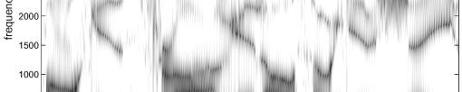
54 Linear Prediction Sectrogram L=8, R=3, N=000, 40 db dynamic range 54

55 Comarison to Other Sectrum Analysis Methods Sectra of synthetic vowel /IY/ (a) Narrowband sectrum using 40 msec window (b) Wideband sectrum using a 0 msec window (c) Cestrally smoothed sectrum (d) LPC sectrum from a 40 msec section using a =2 order LPC analysis 55

56 Comarison to Other Sectrum Analysis Methods Natural seech sectral estimates using cestral smoothing (solid line) and linear rediction analysis (dashed line). Note the fewer (surious) eaks in the LP analysis sectrum since LP used =2 which restricted the sectral match to a maximum of 6 resonance eaks. Note the narrow bandwidths of the LP resonances versus the cestrally smoothed resonances. 56

57 Selective Linear Prediction it is ossible to aly LP methods to selected arts of sectrum - 04kH 0-4 khz for voiced sounds use a redictor of order khz for unvoiced sounds use a redictor of order 2 the key id ea is to ma the frequency region { f, f } linearly to { 0,.} 5 { 2πf 2πf } { 0π} or, equivalently, the region, mas linearly to, via the transformation = ω 2 π f ω A 2πf 2πf 2πf B A ω 2 ω ( ) = j j m R m Sˆ ( ) ω n e e d 2π B we must modify the calculation for the autocorrelation to give: π π A B A B 57

58 Selective Linear Prediction 0-0 khz region modeled using =28 no discontinuity in model sectra at 5 khz 0-5 khz region modeled using =4 5-0 khz region modeled using 2 =5 discontinuity in model sectra at 5 khz 58

59 Solutions of LPC Equations Covariance Method (Cholesky Decomosition Method) 59

60 LPC Solutions-Covariance Method for the covariance method we need to solve the matrix equation αφ k φ ( ik, ) = ( i, 0), i= 2,,..., φα = ψ (in matrix notation) φ is a ositive definite, symmetric matrix with ( i, j) element φ (, i j), and α and ψ are column vectors with elements α and φ ( i, 0) the solution of the matrix equation is called the Cholesky decomosition, or square root method t φ =VDV ; V = lower triangula r matrix ti with ith' 's on the main diagonal D=diagonal matrix i 60

61 LPC Solutions-Covariance Method can readily determine elements of V and D by solving for ( i, j) elements of the matrix equation, as follows giving j ik k jk φ ˆ ( i, j) = V d V, j i n j ij j n ik k jk Vd = φ ˆ ( i, j) V dv, j i and for the diagonal elements giving g φ ˆ ( ii, ) = n i VikdV k ik i d = φ ( i, i) V d, i i with d φ ˆ (, ) = n ik 2 k 2 6

62 Cholesky Decomosition Examle consider examle with = 4, and matrix elements φ ( i, j ) = φ φ φ2 φ3 φ4 φ2 φ22 φ32 φ42 = φ3 φ32 φ33 φ 43 φ 4 φ 42 φ 34 φ d V V V V d V V V3 V d V V4 V42 V d ij 62

63 Cholesky Decomosition Examle solve matrix for d, V, V, V, d, V, V, d, V, d d = φ V d = φ ; V d = φ ; V d = φ V = φ / d ; V = φ / d ; V = φ / d d 2 2 = φ 22 V d 2 ( ) ( φ ) V d = φ V dv V = φ V dv ste ste 2 ste 3 V d = φ V dv V = V dv / d ste 4 / d iterate rocedure to solve for d, V, d

64 LPC Solutions-Covariance Method now need to solve for α using a 2-ste rocedure VDV α = ψ writing this as VY= ψ with t DV α = Y t t or V α = D Y from V (which is now known) solve for column vector Y using a simle recursion of the form i ψ i i ij j j = Y = V Y, i with initial condition Y = ψ 2 64

65 LPC Solutions-Covariance Method now can solve for α using the recursion α i i i ji j j=+ i with initial condition α = = Y / d V α, i Y / d calculation roceeds backwards from i = down to i = 65

66 Cholesky Decomosition Examle continuing the examle we solve for Y Y ψ V2 0 0 Y2 ψ 2 = V3 V32 0 Y 3 ψ 3 V4 V42 V43 Y 4 ψ 4 first solving for Y Y we get Y = ψ Y = ψ V Y Y = ψ V Y V Y Y4 = ψ 4 V4Y V42Y2 V43Y3 66

67 Cholesky Decomosition Examle next solve for α from equation V V V α / d Y Y / d V32 V42 α2 0 / d2 0 0 Y2 Y2 / d2 = = 0 0 V 43 α / d3 0 Y 3 Y3/ d α / d4 Y4 Y4 / d4 giving the results α4 = Y4 / d4 α3 = Y3/ d3 V43α4 α2 = Y2 / d2 V32α3 V42α4 α = Y/ d V2α2 V3α3 V4α4 comleting the solution 67

68 Covariance Method Minimum Error the minimum mean squared error can be written in the form E = φ ( 00, ) α φ ( 0, k) k t = φ (,) 00 α ψ t t since α = YD V can write this as E t 2 k = φ ( 00, ) Y D Y = φ (,) 00 Y / d E n ˆ k this comutation for can be used for all values of LP order from to can understand how LP order reduces mean-squared error 68

69 69

70 Solutions of LPC Equations Autocorrelation Method via Levinson-Durbin Algorithm 70

71 Levinson-Durbin Algorithm i Autocorrelation equations (at each frame ) : αk R[ i k ] = R[ i] i α R=ri is a ositive definite symmetric Toelitz matrix irthe set of otimum redictor coefficients satisfy: Ri [] αk R[ i k ] = 0, i i with minimum mean-squared rediction error of: R[0] α k R [ k ] = E ( ) 7

72 Levinson-Durbin Algorithm 2 i By combining the last two equations we get a larger matrix equation of the form: ( ) R[0] R[] R[2]... R[ ] E ( ) R[] R[0] R[]... R[ ] α 0 ( ) R[2] R[] R[0]... R[ 2] α 2 = ( ) R [ ] R [ ] R [ 2]... R[0] α 0 i exanded matrix is still Toelitz and can be solved iteratively by incororating new correlation value at each iteration and solving for next higher order redictor in terms of new correlation value and revious redictor 72

73 Levinson-Durbin Algorithm 3 th i Show how i order solution can be derived from order solution; i.e., given α, the solution to we derive solution to R α ( i ) ( i ) ( i ) ( i ) ( i ) = e () i () i () i st i The ( i ) solution can be exressed as: R[0] R[] R[2]... R[ i ] E ( i ) R[] R[0] R[]... R[ i 2] α 0 ( i ) R[2] R[] R[0]... R[ i 3] α 2 = ( i ) Ri [ ] Ri [ 2] Ri [ 3]... R[0] α i 0 R α ( i ) st = e 73

74 Levinson-Durbin Algorithm 4 i ( i ) ( i) Aending a 0 to vector α and multilying by the matrix R gives: ( i ) R[0] R[] R[2]... R[ i] E R[] R[0] R[]... R[ i ] ( i ) α 0 ( i ) R[2] R[] R[0]... R[ i 2] α 2 0 = Ri [ ] Ri [ 2] Ri [ 3]... R[] ( i ) α 0 i ( i ) Ri [ ] Ri [ ] Ri [ 2]... R[0] 0 γ i i ( i ) ( i ) α j j= where γ = Ri [] Ri [ j] and Ri [] are introduced 74

75 Levinson-Durbin Algorithm 5 i Key ste is that since Toelitz matrix has secial symmetry we can reverse the order of the equations (first equation last, last equation first), giving: g ( i ) R[0] R[] R[2]... R[ i] 0 γ ( i ) R[] R[0] R[]... R[ i ] α 0 ( i ) R[2] R[] R[0]... R[ i 2] α 2 0 = i ) ( Ri [ ] Ri [ 2] Ri [ 3]... R[] α i 0 ( i ) Ri [] Ri [ ] Ri [ 2]... R[0] E 75

76 Levinson-Durbin Algorithm 6 i To get the equation into the desired form (a single () i e ) comonent in the vector ) we combine the two sets of matrices (with a multilicative factor R i () i ( i ) ( i ) 0 E γ ( ) i α ( i ) α 0 0 ( i ) ( i ) α 2 α ki = ki.... ( i ) α ( i ) i α i 0 0 ( i ) ( i ) 0 γ E ( i ) Choose γ so that non-zero entry, i.e., k i ( i ) Ri [] [ ] ( i ) α j Ri j γ j= i = = ( i ) ( i ) E k i ) giving: vector on right has only a single E 76

77 Levinson-Durbin Algorithm 7 i The first element of the right hand side vector is now: E = E k γ = E ( k ) () i ( i ) ( i ) ( i ) 2 i i i The k arameters are called PARCOR coefficients. i i ( i ) th With this choice of γ, the vector of order coefficients i is: 0 () i ( i ) ( i ) α α α i () i ( i ) ( i ) α 2 α 2 α i 2 = ki... () i ( i ) ( i ) α i αi α () i αi 0 i yielding the udating rocedure α = α kα, j =,2,..., α () i ( i ) ( i ) j j i i j () i i = k i i redictor 77

78 Levinson-Durbin Algorithm 7 i i i i i The final solution for order is: α ( ) j = α j j with rediction error ( ) 2 2 = m = m m= m= E E[0] ( k ) R[0] ( k ) If we use normalized autocorrelation coefficients: rk [ ] = Rk [ ]/ R[0] we get norma lized errors of the form: ν E () i i i () i () i 2 = = αk rk = km R[0] m = () i 0< ν < k i < where or [ ] ( ) 78

79 Levinson-Durbin Algorithm () i ( i ) A ( z) = A ( z) kz A i ( z ) i ( i ) 79

80 Autocorrelation Examle consider a simle = 2 solution of the form R( 0) R() α R() = 0 α R() R( ) R ( 2 ) with solution 2 E ( 0 ) () = R ( 0 ) k = R()/ R( 0) α = R()/ R( 0) 2 2 R 0 R E () = ( ) ( ) R( 0) 80

81 Autocorrelation Examle ( 2) ( 0) ( ) = R R R R ( 0) R ( ) k 2 = 2 2 α α R( 2) R( 0) R ( ) ( 2) 2 = 2 2 R ( 2) = ( 0) R ( ) R() R( 0) R() R( 2) with final coefficients α α E = α ( 2 ) ( 2) 2 = α2 () i R ( 0) R ( ) = rediction error for redictor of order i 8

82 Prediction Error as a Function of V n En Rn[ k] αk R [ 0] R [ 0] = = n n Model order is usually determined by the following rule of thumb: F s /000 oles for vocal tract 2-4 oles for radiation 2 oles for glottal ulse 82

83 Autocorrelation Method Proerties mean-squared rediction error always non-zero decreases monotonically with increasing model order autocorrelation matching roerty model and data match u to order sectrum matching roerty favors eaks of short-time FT minimum-hase roerty zeros of A(z) are inside the unit circle Levinson-Durbin recursion efficient algorithm for finding rediction coefficients PARCOR coefficients and MSE are by-roducts 83