Department of Electrical and Computer Engineering Digital Speech Processing Homework No. 7 Solutions

Transcription

1 Problem 1 Department of Electrical and Computer Engineering Digital Speech Processing Homework No. 7 Solutions Linear prediction analysis is used to obtain an eleventh-order all-pole model for a segment of voiced speech that was sampled at a rate of F S = 8000 samples/second. The system function of the model is: H(z) = G A(z) = G G = α k z k (1 z i z 1 ) k=1 Table 1 shows five of the roots of the eleventh-order prediction error filter, A(z). i z i z i (rad) Table 1: Root locations of eleventh-order prediction error filter in the z-plane. (a) Determine where the other six zeros of A(z) are located in the z-plane. If you cannot precisely determine the pole locations, explain where the pole might occur in the z-plane. (b) Estimate the first three formant frequencies (in Hz) for this segment of speech. (c) Which of the first three formant resonances has the smallest bandwidth? How is this determined? (d) Plot and label the frequency response due to just the first three formants of the all-pole model for the (analog) frequency range 0 f F S /2. Solution (a) Since the five roots of Table 1 are all complex, 5 of the remaining roots occur at the complex conjugate locations. The remaining root must be real and occurs on the z-axis and is generally inside the unit circle. (b) The locations of the formants are determined by the complex roots that are closest to the unit circle, namely with magnitudes close to 1.0. If we order these roots we can estimate the formant frequencies by multiplying the root angle (in radians) by the sampling rate and then dividing by the factor 2π to convert from radians to analog frequency. Using this method we obtain the following formant estimates: i=1 1

2 1. F 1 = (z 3 ) F S /(2π) = /(2π) = 350 Hz 2. F 2 = (z 2 ) F S /(2π) = /(2π) = 1834 Hz 3. F 3 = (z 5 ) F S /(2π) = /(2π) = 3076 Hz There is a choice of the fourth or fifth root as the best estimate of the third formant. However since the fifth root is much closer to the unit circle ( z 5 = ) than the fourth root ( z 4 = ), the fifth root is a better candidate for the third formant. (c) The formant with the smallest bandwidth is the pole which is closest to the unit circle, namely the first formant which has a magnitude of (d) Figure 1 shows a plot of the log magnitude spectrum of the cascade of the first three resonances at the complex pole locations chosen for the three formants, with a transfer function: H(z) = 3 1 2r i cos(θ i ) + ri 2 1 2r i cos(θ i )z 1 + ri 2z 2 i=1 where r i and θ i are the formant magnitudes and angles (in radians) for the first three formants. Figure 1: Plot of log magnitude response of system consisting of 3 formant resonances. Problem 2 An unvoiced speech signal segment can be modeled as a segment of a stationary random process of the form: x[n] = w[n] + βw[n 1] where w[n] is a zero mean, unit variance, stationary white noise process and β < 1. (a) What are the mean and variance of x[n]? (b) What system can be used to recover w[n] from x[n]? 2

3 (c) What is the normalized autocorrelation of x[n] at a delay of 1 sample, i.e., what is r x [1] = R x[1] R x [0]? Solution (a) The mean and variance are calculated as: x[n] = w[n] + bw[n 1] = 0 (since w[n] is a zero-mean process) x 2 [n] = (w[n] + βw[n 1]) 2 = w 2 [n] + 2βw[n] w[n 1] + β 2 w 2 [n 1] = σ 2 w + β 2 σ 2 w = (1 + β 2 )σ 2 w = (1 + β 2 ) (b) The transfer function from w[n] to x[n] is: H 1 (z) = X(z) W (z) = 1 + βz 1 To recover w[n] we need to s x[n] through the inverse system, of the form: (c) The correlation of x[n] is: R x [k] = E{x[n]x[n + k]} H 2 (z) = W (z) X(z) = βz 1 = E{(w[n] + βw[n 1]) (w[n + k] + βw[n + k 1])} = E{w[n]w[n + k]} + βe{w[n 1]w[n + k] + w[n]w[n + k 1]} + β 2 E{w[n 1]w[n + k 1]} = δ[k] + βδ[k 1] + βδ[k + 1] + β 2 δ[k] = (1 + β 2 )δ[k] + βδ[k 1] + βδ[k + 1] giving the final result: r x [1] = R x[1] R x [0] = β 1 + β 2 Problem 3 A causal LTI system has system function: H(z) = 1 4z z z z 3 (a) Use the Levinson recursion to determine whether or not the system is stable. (b) Is the system minimum phase? Solution 3

4 To determine stability, we need to find out if the denominator polynomial has all of its roots inside the unit circle. Consider the denominator polynomial: A(z) = z z z 3 = 1 α (3) 1 z 1 α (3) 2 z 2 α (3) 3 z 3 to be a prediction error filter; therefore we can convert from a i to k i using the backward iteration: k i = a (i) i i = p, p 1,..., 1 α (i 1) j = [α (i) j + α (i) i α (i) i j ]/(1 k2 i ) 1 j i 1 (a) Thus we compute the values of k i using the backward iteration: k 3 = α (3) 3 = α (2) 1 = [α (3) 1 + α (3) 3 α(3) 2 ]/(1 k2 3) = (0.875)(0.75) 1 (0.875) 2 = 3.84 α (2) 2 = [α (3) 2 + α (3) 3 α(3) 1 ]/( (0.875)(0.25) k2 3) = 1 (0.875) 2 = 4.13 k 2 = α (2) 2 = 4.13 α (1) 1 = [α (2) 1 + α (2) 2 α(2) 1 ]/(1 k2 2) = k 1 = α (1) 1 = (4.13)(3.84) 1 (4.13) 2 = 1.23 Since k i > 1 for k 2 and k 1, the system is unstable. (b) The system is not minimum phase since there is a zero at z = 4, which is outside the unit circle, as well as poles outside the unit circle. Problem 4 A speech signal frame (windowed using a Hamming window) has energy: E (0) n = m s 2 n[m] = 2000 Using the autocorrelation method of analysis on this speech frame, the first 3 PARCOR coefficients are computed and their values are: k 1 = 0.5 k 2 = 0.5 k 3 = 0.2 Find the energy of the linear prediction residual, En 3 = e 2 n[m] that would be m obtained by inverse filtering s n [m] by the optimal third order predictor inverse filter, A 3 (z). 4

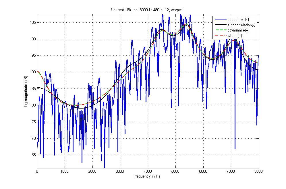
5 Solution The energy of the linear prediction residual using a third order predictor is: E n (3) = E n (0) (1 k1)(1 2 k2)(1 2 k3) 2 = (2000)(1 0.25)(1 0.25)(1 0.04) = 1080 Problem 5 Write a MATLAB program to convert from a frame of speech to a set of linear prediction coefficients, using all 3 methods discussed in class, i.e., the Autocorrelation Method, the Covariance Method, and the Lattice Filter Method. Choose a section of a steady state vowel, and a section of unvoiced speech, and plot LPC spectra from the 3 methods along with the normal spectrum from the Hamming window weighted frame. Use N = 300, p = 12, with Hamming Window weighting for the autocorrelation method. Use the same parameters for the Covariance and Lattice Methods. Use the files ah.wav to get a vowel steady state sound beginning at sample 3000, and the file test 16k.wav to get a fricative beginning at sample (Dont forget that for the covariance and lattice methods, you also need to preserve p samples before the starting sample at n = 3000 for computing correlations, and error signals). Solution The following MATLAB program reads in a file of speech and computes the original spectrum (of the signal weighted by a Hamming window), and plots on top of this the LPC spectrum from the autocorrelation, covariance, and lattice methods. There is a main program and 3 functions (durbin for the autocorrelation method, cholesky for the covariance methodalthough simple matrix inversion was used, rather than the Cholesky decomposition, and lattice for the traditional lattice method). read in speech file, choose section of speech and solve for set of lpc coefficients using the autocorrelation method, the covariance method, and the lattice method plot the resulting spectra from all three methods read in waveform for a speech file [xin,fs,mode,format]=loadwav( ah_truncated.wav );xin) filename=input( enter speech filename:, s ); [xin,fs,mode,format]=loadwav(filename); 5

6 normalize input to [-1,1] range and play out sound file xinn=xin/max(xin); sound(xinn,fs); [nrows ncol]=size(xin); m=input( starting sample for speech frame: ); N=input( frame duration: ); p=input( lpc order: ); wtype=input(window type(1=hamming, 0=Rectangular):); stitle=sprintf( file: s, ss: d N: d p: d,filename,m,n,p); print out number of samples in file, read in plotting parameters fprintf( number of samples in file: 7.0f \n, nrows); autocorrelation method--choose section of speech, window using Hamming window, compute autocorrelation for i=0,1,...,p get original spectrum xino=[(xin(m:m+n-1).*hamming(n)) zeros(1,512-n)]; h0=fft(xino,512); f=0:fs/512:fs-fs/512; plot(f(1:257),20*log10(abs(h0(1:257)))),title(stitle),ylabel( log magnitude (db) ),... xlabel( frequency in Hz ); hold on; autocorrelation method xf=xin(m:m+n-1); [R,E,k,alpha,G]=durbin(xf,N,p,wtype); alphap=alpha(1:p,p); num=[1 -alphap ]; [ha,f]=freqz(g,num,512,fs); plot(f,20*log10(abs(ha)), k- ); fvtool(g,num); covariance method--choose section of speech, compute correlation matrix and covariance vector xc=xin(m-p:m+n-1); [phim,phiv,ec,alphac,gc]=cholesky(xc,n,p); numc=[1 -alphac ]; [hc,f]=freqz(gc,numc,512,fs); plot(f,20*log10(abs(hc)), g-- ); fvtool(gc,numc); lattice method--choose section of speech, compute forward and backward errors xl=xin(m-p:m+n-1); [EL,alphal,GL,k]=lattice(xl,N,p); alphalat=alphal(:,p); numl=[1 -alphalat ]; 6

7 [hl,f]=freqz(gl,numl,512,fs); plot(f,20*log10(abs(hl)), r-. ); leg( windowed speech, autocorrelation method(-), covariance method(--), lattice me fvtool(gl,numl); function [R,E,k,alpha,G]=durbin(xf,N,p,wtype) function [R,E,k,alpha,G]=durbin(xf,N,p,wtype) compute window based on wtype; wtype=1 for Hamming window, wtype=0 for Rectangular window compute R(0:p) from windowed xf solve Durbin recursion fo E,k,alpha in 8 easy steps step 1--E(0)=R(0) step 2--k(1)=R(1)/E(0) step 3--alpha(1,1)=k(1) step 4--E(1)=(1-k(1).^2)E(0) steps 5-8--for i=2,3,...,p; step 5--k(i)=[R(i)-sum from j=1 to i-1 alpha(j,i-1).*r(i-j)]/e(i-1) step 6--alpha(i,i)=k(i) step 7--for j=1,2,...,i-1 alpha(j,i)=alpha(j,i-1)-k(i)alpha(i-j,i-1) step 8--E(i)=(1-k(i).^2)E(i-1) if wtype==1 win=hamming(n); else win=boxcar(n); window frame for autocorrelation method xf=xf.*win; compute autocorrelation for k=0:p R(k+1)=sum(xf(1:N-k).*xf(k+1:N)); solve for lpc coefficients using Durbin s method E=zeros(1,p); k=zeros(1,p); alpha=zeros(p,p); E(1)=R(1); ind=1; k(ind)=r(ind+1)/e(ind); 7

8 alpha(ind,ind)=k(ind); E(ind+1)=(1-k(ind).^2)*E(ind); for ind=2:p k(ind)=(r(ind+1)-sum(alpha(1:ind-1,ind-1).*r(ind:-1:2)))/e(ind); alpha(ind,ind)=k(ind); for jnd=1:ind-1 alpha(jnd,ind)=alpha(jnd,ind-1)-k(ind)*alpha(ind-jnd,ind-1); E(ind+1)=(1-k(ind).^2)*E(ind); G=sqrt(E(p+1)); function [phim,phiv,ec,alphac,gc]=cholesky(xc,n,p) cholesky decomposition first compute phim(1,1)...phim(p,p) next compute phiv(1,0)...phiv(p,0) for i=1:p for k=1:p phim(i,k)=sum(xc(p+1-i:p+n-i).*xc(p+1-k:p+n-k)); for i=1:p phiv(i)=sum(xc(p+1-i:p+n-i).*xc(p+1:p+n)); phiz(i)=sum(xc(p+1:p+n).*xc(p+1-i:p+n-i)); phi0=sum(xc(p+1:p+n).^2); use simple matrix inverse to solve equations--come back to Cholesky decomposition later phiv=phiv ; solve using matrix inverse, phim*alphac=phiv alphac=inv(phim)*phiv alphac=inv(phim)*phiv; EC=phi0-sum(alphac.*phiz); GC=sqrt(EC); function [EL,alphal,GL,k]=lattice(xc,N,p) lattice solution to lpc equations follow 10 step solution step 1--set e(0)(m)=b(0)(m)=s(m) step 2--compute k1=alpha(1,1) from basic lattice reflection coefficient equation 8.89 step 3--determine forward and backward errors e(1)(m) and b(1)(m) from 8

9 eqns 8.84 and 8.87 step 4--set i=2 step 5--determine ki=alpha(i,i) from eqn 8.89 step 6--determine alpha(j,i) for j-1,2,...,i-1 from eqn 8.70 step 7--determine e(i)(m) and b(i)(m) from eqns and 8.87 step 8--set i=i+1 step 9--if i<=p, go to step 5 step 10--finished e(:,1)=xc; b(:,1)=xc; k(1)=sum(e(p+1:p+n,1).*b(p:p+n-1,1))/sqrt((sum(e(p+1:p+n,1).^2)*sum(b(p:p+n-1,1).^2))); alphal(1,1)=k(1); btemp=[0 b(:,1) ] ; e(1:n+p,2)=e(1:n+p,1)-k(1)*btemp(1:n+p); b(1:n+p,2)=btemp(1:n+p)-k(1)*e(1:n+p,1); for i=2:p k(i)=sum(e(p+1:p+n,i).*b(p:p+n-1,i))/sqrt((sum(e(p+1:p+n,i).^2)*sum(b(p:p+n-1,i).^2) alphal(i,i)=k(i); for j=1:i-1 alphal(j,i)=alphal(j,i-1)-k(i)*alphal(i-j,i-1); btemp=[0 b(:,i) ] ; e(1:n+p,i+1)=e(1:n+p,i)-k(i)*btemp(1:n+p); b(1:n+p,i+1)=btemp(1:n+p)-k(i)*e(1:n+p,i); EL=sum(xc(p+1:p+N).^2); for i=1:p EL=EL*(1-k(i).^2); GL=sqrt(EL); The following plots are for a vowel from the file ah.wav, and a fricative from the file test 16k.wav. 9

10 10