5. Atomic radiation processes
|
|
|
- Alexandrina Laura Pierce
- 5 years ago
- Views:
Transcription
1 5. Atomic radiation processes Einstein coefficients for absorption and emission oscillator strength line profiles: damping profile, collisional broadening, Doppler broadening continuous absorption and scattering 1
2 Atomic transitions absorption hν + E l E u emission spontaneous (isotropic) E u E l + hν stimulated (direction of incoming photon) hν + E u E l +2hν 2
3 A. Line transitions Einstein coefficients probability that a photon in frequency interval (ν, ν+dν) in the solid angle range (ω,ω+dω) is absorbed by an atom in the energy level E l with a resulting transition E l E u per second: dw abs (ν, ω,l,u)=b lu I ν (ω) ϕ(ν)dν dω 4π atomic property no. of incident photons probability ν є (ν,ν+dν) probability ω є (ω,ω+dω) absorption profile probability for transition l u B lu : Einstein coefficient for absorption 3
4 Einstein coefficients similarly for stimulated emission dw st (ν,ω,l,u)=b ul I ν (ω) ϕ(ν)dν dω 4π B ul : Einstein coefficient for stimulated emission and for spontaneous emission dw sp (ν, ω,l,u)=a ul ϕ(ν)dν dω 4π A ul : Einstein coefficient for spontaneous emission 4
: stimulated emission")
5 dw st (ν,ω,l,u)=b ul I ν (ω) ϕ(ν)dν dω 4π dw abs (ν, ω,l,u)=b lu I ν (ω) ϕ(ν)dν dω 4π Einstein coefficients, absorption and emission coefficients I df dv = df ds Number of absorptions & stimulated emissions in dv per second: ds n l dw abs dv, n u dw st dv absorbed energy in dv per second: de abs ν = n l hν dw abs dv n u hν dw st dv and also (using definition of intensity): stimulated emission counted as negative absorption de abs ν = κ L ν I ν ds dω dν df κ L ν = hν 4π ϕ(ν) [n lb lu n u B ul ] for the spontaneously emitted energy: Absorption and emission coefficients are a function of Einstein coefficients, occupation numbers and line broadening ² L ν = hν 4π n u A ul ϕ(ν) 5
6 Relations between Einstein coefficients Einstein coefficients are atomic properties do not depend on thermodynamic state of matter We can assume TE: S ν = ²L ν κ L = B ν (T) ν B ν (T) = n u A ul n l B lu n u B ul = n u n l A ul B lu n u n l B ul From the Boltzmann formula: n u n l = g u e hν kt g l for h/kt << 1: n u n l = g u g l µ 1 hν, B kt ν (T) = 2ν2 c 2 kt 2ν 2 c 2 kt = g u g l µ 1 hν kt B lu g u g l A ul 1 hν kt Bul for T 1 0 g l B lu = g u B ul 6
7 2ν 2 c 2 kt = g µ u 1 hν g l kt B lu g u gl A ul 1 hν kt Bul g l B lu = g u B ul Relations between Einstein coefficients 2ν 2 c 2 kt = g µ u 1 hν Aul kt g l kt B lu hν 2 hν 3 c 2 = A ul B lu g u g l µ 1 hν kt for T 1 A ul = 2 h ν 3 A ul = c 2 2h ν3 c 2 κ L ν = hν 4π ϕ(ν) B lu ² L ν = hν 4π ϕ(ν) n u g l g u B lu B ul n l g l n g u u g l 2hν 3 g u c 2 B lu Note: Einstein coefficients atomic quantities. That means any relationship that holds in a special thermodynamic situation (such as T very large) must be generally valid. only one Einstein coefficient needed 7
8 Oscillator strength Quantum mechanics The Einstein coefficients can be calculated by quantum mechanics + classical electrodynamics calculation. Eigenvalue problem using using wave function: H atom ψ l >= E l ψ l > H atom = p2 2m + V nucleus + V shell Consider a time-dependent perturbation such as an external electromagnetic field (light wave) E(t) = E 0 e it. The potential of the time dependent perturbation on the atom is: NX V (t)=e E r i = E d i=1 [H atom + V (t)] ψ l >= E l ψ l > d: dipol operator with transition probability < ψ l d ψ u > 2 8
9 Oscillator strength The result is hν 4π B lu = πe2 m e c f lu f lu : oscillator strength (dimensionless) classical result from electrodynamics = cm 2 /s Classical electrodynamics electron quasi-elastically bound to nucleus and oscillates within outer electric field as E. Equation of motion (damped harmonic oscillator): ẍ + γẋ + ω 2 0x = e m e E ma = damping force + restoring force + EM force damping constant γ = 2 ω2 0e 2 3 m e c = 8π 2 e 2 ν m e c 3 resonant (natural) frequency ω 0 =2πν 0 the electron oscillates preferentially at resonance (incoming radiation ν = ν 0 ) The damping is caused, because the de- and accelerated electron radiates 9
10 Classical cross section and oscillator strength Calculating the power absorbed by the oscillator, the integrated classical absorption coefficient and cross section, and the absorption line profile are found: Z integrated over the line profile κ L,cl ν dν = n l πe 2 m e c = n l σ cl tot n l : number density of absorbers σ tot cl : classical cross section (cm 2 /s) ϕ(ν)dν = 1 π γ/4π (ν ν 0 ) 2 +(γ/4π) 2 [Lorentz (damping) line profile] oscillator strength f lu is quantum mechanical correction to classical result (effective number of classical oscillators, 1 for strong resonance lines) From κ L ν = hν 4π ϕ(ν) n lb lu (neglecting stimulated emission) 10
11 Oscillator strength hν 4π ϕ(ν) B lu = πe2 m e c ϕ(ν) f lu = σ lu (ν) absorption cross section; dimension is cm 2 /s f lu = 1 4π m e c πe 2 hν B lu Oscillator strength (f-value) is different for each atomic transition Values are determined empirically in the laboratory or by elaborate numerical atomic physics calculations Semi-analytical calculations possible in simplest cases, e.g. hydrogen f lu = 25 g /2 π l 5 u 3 l 2 u 2 g: Gaunt factor Hα: f= Hβ: f= Hγ: f=
12 Line profiles line profiles contain information on physical conditions of the gas and chemical abundances analysis of line profiles requires knowledge of distribution of opacity with frequency several mechanisms lead to line broadening (no infinitely sharp lines) - natural damping: finite lifetime of atomic levels - collisional (pressure) broadening: impact vs quasi-static approximation - Doppler broadening: convolution of velocity distribution with atomic profiles 12
13 1. Natural damping profile finite lifetime of atomic levels line width NATURAL LINE BROADENING OR RADIATION DAMPING τ = 1 / A ul Δ E τ h/2π ( 10-8 s in H atom 2 1): finite lifetime with respect to spontaneous emission uncertainty principle ϕ(ν) = 1 π line broadening Γ/4π (ν ν 0 ) 2 +(Γ/4π) 2 Δν 1/2 = Γ / 2π Δλ 1/2 = λ 2 Γ / 2πc e.g. Ly α: Δλ 1/2 = A Hα: Δλ 1/2 = A Lorentzian profile 13
14 Natural damping profile resonance line Γ u = i<u A ui Γ = A u1 Γ l = i<l A li Γ = Γ u + Γ l natural line broadening is important for strong lines (resonance lines) at low densities (no additional broadening mechanisms) e.g. Ly α in interstellar medium but also in stellar atmospheres 14
15 2. Collisional broadening radiating atoms are perturbed by the electromagnetic field of neighbour atoms, ions, electrons, molecules energy levels are temporarily modified through the Stark - effect: perturbation is a function of separation absorber-perturber energy levels affected line shifts, asymmetries & broadening ΔE(t) = h Δν = C/r n (t) r: distance to perturbing atom a) impact approximation: radiating atoms are perturbed by passing particles at distance r(t). Duration of collision << lifetime in level lifetime shortened line broader in all cases a Lorentzian profile is obtained (but with larger total Γ than only natural damping) b) quasi-static approximation: applied when duration of collisions >> life time in level consider stationary distribution of perturbers 15
16 Collisional broadening n = 2 linear Stark effect ΔE» F for levels with degenerate angular momentum (e.g. HI, HeII) field strength F» 1/r 2 ΔE» 1/r 2 important for H I lines, in particular in hot stars (high number density of free electrons and ions). However, for ion collisional broadening the quasi-static broadening is also important for strong lines (see below) n = 3 resonance broadening atom A perturbed by atom A of same species important in cool stars, e.g. Balmer lines in the Sun ΔE» 1/r 3 16
17 Collisional broadening n = 4 quadratic Stark effect ΔE F 2 field strength F 1/r 2 ΔE 1/r 4 (no dipole moment) important for metal ions broadened by e - in hot stars Lorentz profile with γ e ~ n e n = 6 van der Waals broadening atom A perturbed by atom B important in cool stars, e.g. Na perturbed by H in the Sun 17
18 Quasi-static approximation t perturbation >> τ = 1/A ul perturbation practically constant during emission or absorption atom radiates in a statistically fluctuating field produced by quasi-static perturbers, e.g. slow-moving ions given a distribution of perturbers field at location of absorbing or emitting atom statistical frequency of particle distribution probability of fields of different strength (each producing an energy shift ΔE = h Δν) field strength distribution function line broadening Linear Stark effect of H lines can be approximated to 0 st order in this way 18
19 Quasi-static approximation for hydrogen line broadening Line broadening profile function determined by probability function for electric field caused by all other particles as seen by the radiating atom. W(F) df: probability that field seen by radiating atom is F ϕ( ν) dν = W (F ) df dν dν For calculating W(F)dF we use as a first step the nearest-neighbor approximation: main effect from nearest particle 19
20 Quasi-static approximation nearest neighbor approximation assumption: main effect from nearest particle (F ~ 1/r 2 ) we need to calculate the probability that nearest neighbor is in the distance range (r,r+dr) = probability that none is at distance < r and one is in (r,r+dr) W(r) dr =[1 Z r 0 W (x) dx] (4πr 2 N) dr Integral equation for W(r) we find solution by differentiating differential equation probability for no particle in (0,r) relative probability for particle in shell (r,r+dr) N: total uniform particle density d dr W(r) 4πr 2 = W (r) = 4πr 2 N N W (r) 4πr 2 N Differential equation W (r)=4πr 2 Ne 4 3 πr3 N Normalized solution 20
21 Quasi-static approximation mean interparticle distance: normal field strength: r 0 = F 0 = e r 2 0 µ 4 1/3 3 π N (linear Stark) W (r)dr = e r 3 r 3 r 0 d{ } r 0 define: β = F F 0 = { r 0 r }2 note: at high particle density large F 0 stronger broadening from W(r) dr W(β) dβ: W (β)dβ = 3 2 β 5/2 e β 3/2 dβ W (β ) β 5/2 for β ν β ϕ( ν) ν 5/2 Stark broadened line profile in the wings, not Δλ -2 as for natural or impact broadening 21
22 Quasi-static approximation advanced theory complete treatment of an ensemble of particles: Holtsmark theory + interaction among perturbers (Debye shielding of the potential at distances > Debye length) Holtsmark (1919), Chandrasekhar (1943, Phys. Rev. 15, 1) W (β) = 2β π Z 0 e y3/2 ysin(βy)dy number of particles inside Debye sphere Ecker (1957, Zeitschrift f. Physik, 148, 593 & 149,245) Z W (β) = 2βδ4/3 π 0 e δg(y) ysin(δ 2/3 βy)dy g(y) = 2 Z 3 y3/2 (1 z 1 sinz)z 5/2 dz y D =4.8 T n e 1/2cm Debye length, field of ion vanishes beyond D Mihalas, 78 δ = 4π 3 D3 N number of particles inside Debye sphere 22
23 3. Doppler broadening radiating atoms have thermal velocity Maxwellian distribution: P (v x,v y,v z ) dv x dv y dv z = ³ m 3/2 e m 2kT (v2 x +v2 y +v2 z ) dv x dv y dv z 2πkT Doppler effect: atom with velocity v emitting at frequency ν 0, observed at frequency ν: ν 0 = ν ν v cos θ c 23
24 Doppler broadening Define the velocity component along the line of sight: ξ The Maxwellian distribution for this component is: P (ξ) dξ = 1 π 1/2 ξ 0 e ξ ξ0 2 dξ ξ 0 =(2kT /m) 1/2 thermal velocity ν 0 = ν ν ξ c if we observe at ν, an atom with velocity component ξ absorbs at ν 0 in its frame if v/c <<1 (ν 0 -ν)/ν <<1: line center ν = ν 0 ν = ν ξ c = [(ν ν 0)+ν 0 ] ξ c ν 0 ξ c 24
25 Doppler broadening line profile for v = 0 profile for v 0 ν ν 0 ϕ R (ν ν 0 ) = ϕ R (ν 0 ν 0 )=ϕ(ν ν 0 ν 0 ξ c ) New line profile: convolution ϕ new (ν ν 0 )= Z ξ ϕ(ν ν 0 ν 0 ) P (ξ) dξ c profile function in rest frame velocity distribution function 25
26 Doppler broadening: sharp line approximation ϕ new (ν ν 0 )= 1 π 1/2 Z ϕ(ν ν 0 ν 0 ξ 0 c ξ ) e ξ 2 ξ 0 ξ 0 dξ ξ 0 Δν D : Doppler width of the line Δν D = ν (T/μ) 1/2 Δλ D = λ (T/μ) 1/2 ξ 0 =(2kT/m) 1/2 thermal velocity Approximation 1: assume a sharp line half width of profile function << Δν D ϕ(ν ν 0 ) δ(ν ν 0 ) delta function 26
27 Doppler broadening: sharp line approximation ϕ new (ν ν 0 )= 1 π 1/2 Z δ(ν ν 0 ν D ξ ) e ξ 2 ξ 0 ξ 0 dξ ξ 0 δ(a x)= 1 a δ(x) ϕ new (ν ν 0 )= 1 π 1/2 Z µ ν ν0 δ ξ ν D ξ 0 e ξ ξ0 2 dξ ν D ξ 0 ϕ new (ν ν 0 )= 1 π 1/ 2 ν D e ν ν0 νd 2 Gaussian profile valid in the line core 27
28 Doppler broadening: Voigt function Approximation 2: assume a Lorentzian profile half width of profile function > Δν D ϕ(ν) = 1 π Γ/4π (ν ν 0 ) 2 +(Γ/4π) 2 ϕ new (ν ν 0 )= 1 π 1/2 ν D a π Z e y 2 ³ 2 ν ν D y + a 2 dy a = Γ 4π ν D ϕ new (ν ν 0 )= 1 π 1/2 ν D H µ a, ν ν 0 ν D Voigt function (Lorentzian * Gaussian): calculated numerically 28
29 Doppler broadening: Voigt function H Approximate representation of Voigt function: ³ a, ν ν 0 ν D e ν ν0 νd 2 line core: Doppler broadening a π 1/2 ν ν0 νd 2 line wings: damping profile only visible for strong lines General case: for any intrinsic profile function (Lorentz, or Holtsmark, etc.) the observed profile is obtained from numerical convolution with the different broadening functions and finally with Doppler broadening 29
30 Voigt function normalization: Z H(a, v) dv = π usually α <<1 max at v=0: H(α,v=0) 1-α ~ Gaussian ~ Lorentzian Unsoeld, 68 30
31 B. Continuous transitions 1. Bound-free and free-free processes absorption hν + E l E u photoionization - recombination hν lk emission spontaneous (isotropic) stimulated (non-isotropic) E u E l + hν hν + E u E l +2hν bound-bound: spectral lines bound-free κ cont free-free ν consider photon hν hν lk (energy > threshold): extra-energy to free electron e.g. Hydrogen 1 2 mv2 = hν hc R n 2 R = Rydberg constant = cm -1 31
32 b-f and f-f processes Hydrogen Transition l u Wavelength (A) Edge Lyman Balmer Paschen Brackett Pfund 32
33 b-f and f-f processes - for a single transition κ b f ν = n l σ lk (ν) - for all transitions: κ b f ν = X X n l σ lk (ν) elements, ions l Gaunt factor 1 for hydrogenic ions for H: σ 0 = n σ lk (ν) =σ 0 (n) ³ νl 3 gbf (ν) ν Kramers 1923 Gray, 92 ν l = / n 2 extinction per particle 33
34 b-f and f-f processes Gray, 92 late A σ b-f n (ν) = Z 4 n 5 ν 3 g bf (ν) peaks increase with n: hν n = E E n =13.6/n 2 ev = ν 3 n 6 late B for non-h-like atoms no ν -3 dependence peaks at resonant frequencies free-free absorption much smaller 34
35 b-f and f-f processes Hydrogen dominant continuous absorber in B, A & F stars (later stars H - ) Energy distribution strongly modulated at the edges: Balmer Paschen Vega Brackett 35
36 b-f and f-f processes : Einstein-Milne relations Generalize Einstein relations to bound-free processes relating photoionizations and radiative recombinations line transitions σ lu (ν) = hν 4π ϕ(ν) B lu g l B lu = g u B ul A ul = 2h ν3 c 2 B ul b-f transitions κ b f ν = X elements, ions " X σ ik (ν) n i n e n Ion 1 i g i 2g 1 stimulated b-f emission µ h 2 2πmkT n i 3/2 e Ei Ion /kt e hν /kt # LTE occupation number 36
37 2. Scattering In scattering events photons are not destroyed, but redirected and perhaps shifted in frequency. In free-free process photon interacts with electron in the presence of ion s potential. For scattering there is no influence of ion s presence. in general: κ sc = n e σ e Calculation of cross sections for scattering by free electrons: - very high energy (several MeV s): Klein-Nishina formula (Q.E.D.) - high energy photons (electrons): Compton (inverse Compton) scattering - low energy (< 12.4 kev ' 1 Angstrom): Thomson scattering 37
38 Thomson scattering THOMSON SCATTERING: important source of opacity in hot OB stars σ e = 8π 3 r2 0 = 8π 3 e 4 m 2 e c4 = cm 2 independent of frequency, isotropic Approximations: - angle averaging done, in reality: σ e σ e (1+cos 2 φ) for single scattering - neglected velocity distribution and Doppler shift (frequency-dependency) 38
39 Rayleigh scattering RAYLEIGH SCATTERING: line absorption/emission of atoms and molecules far from resonance frequency: ν << ν 0 from classical expression of cross section for oscillators: σ(ω) =f ij σ kl (ω)=f ij σ e ω 4 (ω 2 ω 2 ij )2 + ω 2 γ 2 ω 4 for ω << ω ij σ(ω) f ij σ e ω 4 ij + ω2 γ 2 ω 4 for γ << ω ij σ(ω) f ij σ e σ(ω) ω 4 λ 4 ω 4 ij important in cool G-K stars for strong lines (e.g. Lyman series when H is neutral) the λ -4 decrease in the far wings can be important in the optical 39
40 What are the dominant elements for the continuum opacity? - hot stars (B,A,F) : H, He I, He II - cool stars (G,K): the bound state of the H - ion (1 proton + 2 electrons) The H - ion only way to explain solar continuum (Wildt 1939) ionization potential = ev λ ion = Angstroms H - b-f peaks around 8500 A H - f-f ~ λ 3 (IR important) He - b-f negligible, He - f-f can be important in cool stars in IR requires metals to provide source of electrons dominant source of b-f opacity in the Sun Gray, 92 40
41 Additional continuous absorbers Hydrogen H 2 molecules more numerous than atomic H in M stars H 2+ absorption in UV H 2- f-f absorption in IR Helium He - f-f absorption for cool stars Metals C, Si, Al, Mg, Fe: b-f absorption in UV 41
42 Examples of continuous absorption coefficients Unsoeld, 68 T eff = 5040 K B0: T eff = 28,000 K 42
43 Summary Total opacity κ ν = NX i=1 NX j=i+1 σ line ij µ (ν) n i g i n j g j line absorption + NX i=1 σ ik (ν) ³n i n ie hν/kt +n e n p σ kk (ν,t) +n e σ e hν /kt ³1 e bound-free free-free Thomson scattering 43
44 Summary Total emissivity ² ν = 2hν 3 c 2 + 2hν 3 c 2 NX NX i=1 j=i+1 σij line (ν) g i n j g j NX n iσ ik (ν)e hν/kt i=1 line emission bound-free + 2hν3 c 2 +n e σ e J ν n e n p σ kk (ν,t)e hν/kt free-free Thomson scattering 44
45 Summary Modern model atmosphere codes include: millions of spectral lines all bf- and ff-transitions of hydrogen helium and metals contributions of all important negative ions molecular opacities 45
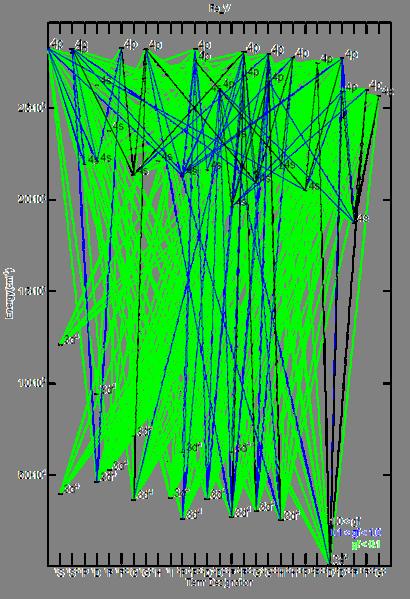
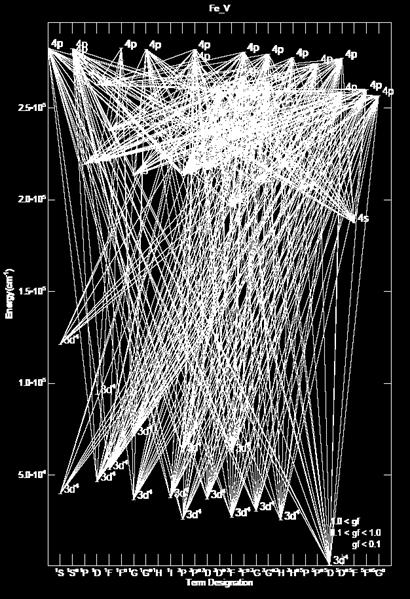

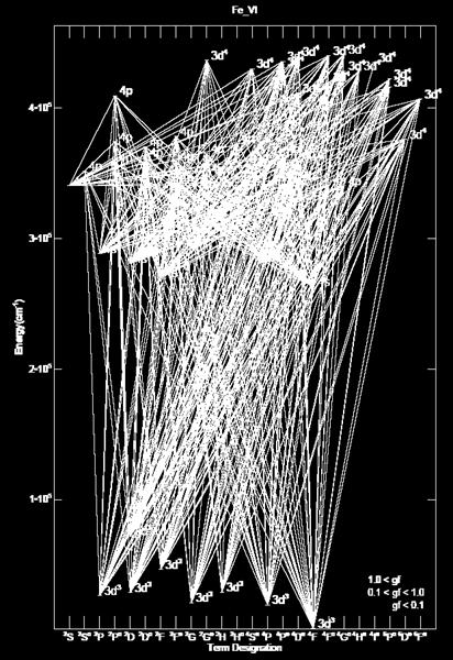
46 Concepcion 2007 complex atomic models for O-stars (Pauldrach et al., 2001) 46
 20,000diel. rec.")
47 NLTE Atomic Models in modern model atmosphere codes lines, collisions, ionization, recombination Essential for occupation numbers, line blocking, line force Accurate atomic models have been included 26 elements 149 ionization stages 5,000 levels ( + 100,000 ) 20,000diel. rec. transitions b-b line transitions Auger-ionization recently improved models are based on Superstructure Eisner et al., 1974, CPC 8,270 AWAP 05/19/05 47
48 Concepcion
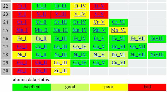
49 Recent Improvements on Atomic Data requires solution of Schrödinger equation for N-electron system efficient technique: R-matrix method in CC approximation Opacity Project Seaton et al. 1994, MNRAS, 266, 805 IRON Project Hummer et al. 1993, A&A, 279, 298 accurate radiative/collisional data to 10% on the mean 49


50 Confrontation with Reality Photoionization Electron Collision Nahar 2003, ASP Conf. Proc.Ser. 288, in press Williams 1999, Rep. Prog. Phys., 62, 1431 high-precision atomic data 50


51 Improved Modelling for Astrophysics e.g. photoionization cross-sections for carbon model atom 51 Przybilla, Butler & Kudritzki 2001b, A&A, 379, 936
5. Atomic radiation processes
 5. Atomic radiation processes Einstein coefficients for absorption and emission oscillator strength line profiles: damping profile, collisional broadening, Doppler broadening continuous absorption and
5. Atomic radiation processes
 5. Atomic radiation processes Einstein coefficients for absorption and emission oscillator strength line profiles: damping profile, collisional broadening, Doppler broadening continuous absorption and
7. Non-LTE basic concepts
 7. Non-LTE basic concepts LTE vs NLTE occupation numbers rate equation transition probabilities: collisional and radiative examples: hot stars, A supergiants 1 Equilibrium: LTE vs NLTE LTE each volume
3. Stellar Atmospheres: Opacities
 3. Stellar Atmospheres: Opacities 3.1. Continuum opacity The removal of energy from a beam of photons as it passes through matter is governed by o line absorption (bound-bound) o photoelectric absorption
The Stellar Opacity. F ν = D U = 1 3 vl n = 1 3. and that, when integrated over all energies,
 The Stellar Opacity The mean absorption coefficient, κ, is not a constant; it is dependent on frequency, and is therefore frequently written as κ ν. Inside a star, several different sources of opacity
7. Non-LTE basic concepts
 7. Non-LTE basic concepts LTE vs NLTE occupation numbers rate equation transition probabilities: collisional and radiative examples: hot stars, A supergiants 10/13/2003 Spring 2016 LTE LTE vs NLTE each
Spontaneous Emission, Stimulated Emission, and Absorption
 Chapter Six Spontaneous Emission, Stimulated Emission, and Absorption In this chapter, we review the general principles governing absorption and emission of radiation by absorbers with quantized energy
6. Stellar spectra. excitation and ionization, Saha s equation stellar spectral classification Balmer jump, H -
 6. Stellar spectra excitation and ionization, Saha s equation stellar spectral classification Balmer jump, H - 1 Occupation numbers: LTE case Absorption coefficient: = n i calculation of occupation numbers
Lecture 2 Line Radiative Transfer for the ISM
 Lecture 2 Line Radiative Transfer for the ISM Absorption lines in the optical & UV Equation of transfer Absorption & emission coefficients Line broadening Equivalent width and curve of growth Observations
6. Stellar spectra. excitation and ionization, Saha s equation stellar spectral classification Balmer jump, H -
 6. Stellar spectra excitation and ionization, Saha s equation stellar spectral classification Balmer jump, H - 1 Occupation numbers: LTE case Absorption coefficient: = n i calculation of occupation numbers
Lecture 10. Lidar Effective Cross-Section vs. Convolution
 Lecture 10. Lidar Effective Cross-Section vs. Convolution q Introduction q Convolution in Lineshape Determination -- Voigt Lineshape (Lorentzian Gaussian) q Effective Cross Section for Single Isotope --
Quantum Electronics/Laser Physics Chapter 4 Line Shapes and Line Widths
 Quantum Electronics/Laser Physics Chapter 4 Line Shapes and Line Widths 4.1 The Natural Line Shape 4.2 Collisional Broadening 4.3 Doppler Broadening 4.4 Einstein Treatment of Stimulated Processes Width
Lecture 6: Continuum Opacity and Stellar Atmospheres
 Lecture 6: Continuum Opacity and Stellar Atmospheres To make progress in modeling and understanding stellar atmospheres beyond the gray atmosphere, it is necessary to consider the real interactions between
3: Interstellar Absorption Lines: Radiative Transfer in the Interstellar Medium. James R. Graham University of California, Berkeley
 3: Interstellar Absorption Lines: Radiative Transfer in the Interstellar Medium James R. Graham University of California, Berkeley Interstellar Absorption Lines Example of atomic absorption lines Structure
Lecture Notes on Radiation Transport for Spectroscopy
 Lecture Notes on Radiation Transport for Spectroscopy ICTP-IAEA School on Atomic Processes in Plasmas 27 February 3 March 217 Trieste, Italy LLNL-PRES-668311 This work was performed under the auspices
Lecture 2 Interstellar Absorption Lines: Line Radiative Transfer
 Lecture 2 Interstellar Absorption Lines: Line Radiative Transfer 1. Atomic absorption lines 2. Application of radiative transfer to absorption & emission 3. Line broadening & curve of growth 4. Optical/UV
Electromagnetic Spectra. AST443, Lecture 13 Stanimir Metchev
 Electromagnetic Spectra AST443, Lecture 13 Stanimir Metchev Administrative Homework 2: problem 5.4 extension: until Mon, Nov 2 Reading: Bradt, chapter 11 Howell, chapter 6 Tenagra data: see bottom of Assignments
The Formation of Spectral Lines. I. Line Absorption Coefficient II. Line Transfer Equation
 The Formation of Spectral Lines I. Line Absorption Coefficient II. Line Transfer Equation Line Absorption Coefficient Main processes 1. Natural Atomic Absorption 2. Pressure Broadening 3. Thermal Doppler
Thermal Equilibrium in Nebulae 1. For an ionized nebula under steady conditions, heating and cooling processes that in
 Thermal Equilibrium in Nebulae 1 For an ionized nebula under steady conditions, heating and cooling processes that in isolation would change the thermal energy content of the gas are in balance, such that
PHYS 231 Lecture Notes Week 3
 PHYS 231 Lecture Notes Week 3 Reading from Maoz (2 nd edition): Chapter 2, Sec. 3.1, 3.2 A lot of the material presented in class this week is well covered in Maoz, and we simply reference the book, with
Interaction of Molecules with Radiation
 3 Interaction of Molecules with Radiation Atoms and molecules can exist in many states that are different with respect to the electron configuration, angular momentum, parity, and energy. Transitions between
X-ray Radiation, Absorption, and Scattering
 X-ray Radiation, Absorption, and Scattering What we can learn from data depend on our understanding of various X-ray emission, scattering, and absorption processes. We will discuss some basic processes:
6. Stellar spectra. excitation and ionization, Saha s equation stellar spectral classification Balmer jump, H -
 6. Stellar spectra excitation and ionization, Saha s equation stellar spectral classification Balmer jump, H - 1 Occupation numbers: LTE case Absorption coefficient: κ ν = n i σ ν$ à calculation of occupation
Astronomy 421. Lecture 14: Stellar Atmospheres III
 Astronomy 421 Lecture 14: Stellar Atmospheres III 1 Lecture 14 - Key concepts: Spectral line widths and shapes Curve of growth 2 There exists a stronger jump, the Lyman limit, occurring at the wavelength
Stellar atmospheres: an overview
 Stellar atmospheres: an overview Core M = 2x10 33 g R = 7x10 10 cm 50 M o 20 R o L = 4x10 33 erg/s 10 6 L o 10 4 (PN) 10 6 (HII) 10 12 (QSO) L o Photosphere Envelope Chromosphere/Corona R = 200 km ~ 3x10
Diffuse Interstellar Medium
 Diffuse Interstellar Medium Basics, velocity widths H I 21-cm radiation (emission) Interstellar absorption lines Radiative transfer Resolved Lines, column densities Unresolved lines, curve of growth Abundances,
Spectroscopy Applied to Selected Examples
 Spectroscopy Applied to Selected Examples Radial Velocities Exoplanets λ obs λ rest λ rest = Δλ λ rest v c for z
(c) Sketch the ratio of electron to gas pressure for main sequence stars versus effective temperature. [1.5]
![(c) Sketch the ratio of electron to gas pressure for main sequence stars versus effective temperature. [1.5]](/thumbs/77/76458229.jpg "(c) Sketch the ratio of electron to gas pressure for main sequence stars versus effective temperature. [1.5]") 1. (a) The Saha equation may be written in the form N + n e N = C u+ u T 3/2 exp ( ) χ kt where C = 4.83 1 21 m 3. Discuss its importance in the study of stellar atmospheres. Carefully explain the meaning
1. (a) The Saha equation may be written in the form N + n e N = C u+ u T 3/2 exp ( ) χ kt where C = 4.83 1 21 m 3. Discuss its importance in the study of stellar atmospheres. Carefully explain the meaning
(c) (a) 3kT/2. Cascade
 (a) 3kT/2. Cascade") 1 AY30-HIITemp IV. Temperature of HII Regions A. Motivations B. History In star-forming galaxies, most of the heating + cooling occurs within HII regions Heating occurs via the UV photons from O and B
1 AY30-HIITemp IV. Temperature of HII Regions A. Motivations B. History In star-forming galaxies, most of the heating + cooling occurs within HII regions Heating occurs via the UV photons from O and B
Spectroscopy Lecture 2
 Spectroscopy Lecture 2 I. Atomic excitation and ionization II. Radiation Terms III. Absorption and emission coefficients IV. Einstein coefficients V. Black Body radiation I. Atomic excitation and ionization
Theory of optically thin emission line spectroscopy
 Theory of optically thin emission line spectroscopy 1 Important definitions In general the spectrum of a source consists of a continuum and several line components. Processes which give raise to the continuous
Plasma Spectroscopy Inferences from Line Emission
 Plasma Spectroscopy Inferences from Line Emission Ø From line λ, can determine element, ionization state, and energy levels involved Ø From line shape, can determine bulk and thermal velocity and often
Photoionized Gas Ionization Equilibrium
 Photoionized Gas Ionization Equilibrium Ionization Recombination H nebulae - case A and B Strömgren spheres H + He nebulae Heavy elements, dielectronic recombination Ionization structure 1 Ionization Equilibrium
Atomic Structure and Processes
 Chapter 5 Atomic Structure and Processes 5.1 Elementary atomic structure Bohr Orbits correspond to principal quantum number n. Hydrogen atom energy levels where the Rydberg energy is R y = m e ( e E n
M.Phys., M.Math.Phys., M.Sc. MTP Radiative Processes in Astrophysics and High-Energy Astrophysics
 M.Phys., M.Math.Phys., M.Sc. MTP Radiative Processes in Astrophysics and High-Energy Astrophysics Professor Garret Cotter garret.cotter@physics.ox.ac.uk Office 756 in the DWB & Exeter College Radiative
Electrodynamics of Radiation Processes
 Electrodynamics of Radiation Processes 7. Emission from relativistic particles (contd) & Bremsstrahlung http://www.astro.rug.nl/~etolstoy/radproc/ Chapter 4: Rybicki&Lightman Sections 4.8, 4.9 Chapter
Overview of Astronomical Concepts III. Stellar Atmospheres; Spectroscopy. PHY 688, Lecture 5 Stanimir Metchev
 Overview of Astronomical Concepts III. Stellar Atmospheres; Spectroscopy PHY 688, Lecture 5 Stanimir Metchev Outline Review of previous lecture Stellar atmospheres spectral lines line profiles; broadening
Opacity and Optical Depth
 Opacity and Optical Depth Absorption dominated intensity change can be written as di λ = κ λ ρ I λ ds with κ λ the absorption coefficient, or opacity The initial intensity I λ 0 of a light beam will be
Interstellar Astrophysics Summary notes: Part 2
 Interstellar Astrophysics Summary notes: Part 2 Dr. Paul M. Woods The main reference source for this section of the course is Chapter 5 in the Dyson and Williams (The Physics of the Interstellar Medium)
Atomic Spectral Lines
 Han Uitenbroek National Solar Observatory/Sacramento Peak Sunspot, USA Hale COLLAGE, Boulder, Feb 18, 216 Today s Lecture How do we get absorption and emission lines in the spectrum? Atomic line- and continuum
Atomic Physics 3 ASTR 2110 Sarazin
 Atomic Physics 3 ASTR 2110 Sarazin Homework #5 Due Wednesday, October 4 due to fall break Test #1 Monday, October 9, 11-11:50 am Ruffner G006 (classroom) You may not consult the text, your notes, or any
CHAPTER 22. Astrophysical Gases
 CHAPTER 22 Astrophysical Gases Most of the baryonic matter in the Universe is in a gaseous state, made up of 75% Hydrogen (H), 25% Helium (He) and only small amounts of other elements (called metals ).
Ay Fall 2004 Lecture 6 (given by Tony Travouillon)
") Ay 122 - Fall 2004 Lecture 6 (given by Tony Travouillon) Stellar atmospheres, classification of stellar spectra (Many slides c/o Phil Armitage) Formation of spectral lines: 1.excitation Two key questions:
Ay 122 - Fall 2004 Lecture 6 (given by Tony Travouillon) Stellar atmospheres, classification of stellar spectra (Many slides c/o Phil Armitage) Formation of spectral lines: 1.excitation Two key questions:
Emitted Spectrum Summary of emission processes Emissivities for emission lines: - Collisionally excited lines - Recombination cascades Emissivities
 Emitted Spectrum Summary of emission processes Emissivities for emission lines: - Collisionally excited lines - Recombination cascades Emissivities for continuum processes - recombination - brehmsstrahlung
Stellar Astrophysics: The Interaction of Light and Matter
 Stellar Astrophysics: The Interaction of Light and Matter The Photoelectric Effect Methods of electron emission Thermionic emission: Application of heat allows electrons to gain enough energy to escape
Absorption Line Physics
 Topics: 1. Absorption line shapes 2. Absorption line strength 3. Line-by-line models Absorption Line Physics Week 4: September 17-21 Reading: Liou 1.3, 4.2.3; Thomas 3.3,4.4,4.5 Absorption Line Shapes
Substellar Atmospheres II. Dust, Clouds, Meteorology. PHY 688, Lecture 19 Mar 11, 2009
 Substellar Atmospheres II. Dust, Clouds, Meteorology PHY 688, Lecture 19 Mar 11, 2009 Outline Review of previous lecture substellar atmospheres: opacity, LTE, chemical species, metallicity Dust, Clouds,
The Curve of Growth of the Equivalent Width
 9 The Curve of Growth of the Equivalent Width Spectral lines are broadened from the transition frequency for a number of reasons. Thermal motions and turbulence introduce Doppler shifts between atoms and
Opacity. requirement (aim): radiative equilibrium: near surface: Opacity
: radiative equilibrium: near surface: Opacity") (Gray) Diffusion approximation to radiative transport: (assumes isotropy valid only in the deep stellar interior) - opacity is a function of frequency (wave length ). - aim: to reduce the (rather complex)
(Gray) Diffusion approximation to radiative transport: (assumes isotropy valid only in the deep stellar interior) - opacity is a function of frequency (wave length ). - aim: to reduce the (rather complex)
Spectral Line Shapes. Line Contributions
 Spectral Line Shapes Line Contributions The spectral line is termed optically thin because there is no wavelength at which the radiant flux has been completely blocked. The opacity of the stellar material
Stars AS4023: Stellar Atmospheres (13) Stellar Structure & Interiors (11)
 Stellar Structure & Interiors (11)") Stars AS4023: Stellar Atmospheres (13) Stellar Structure & Interiors (11) Kenneth Wood, Room 316 kw25@st-andrews.ac.uk http://www-star.st-and.ac.uk/~kw25 What is a Stellar Atmosphere? Transition from dense
Stars AS4023: Stellar Atmospheres (13) Stellar Structure & Interiors (11) Kenneth Wood, Room 316 kw25@st-andrews.ac.uk http://www-star.st-and.ac.uk/~kw25 What is a Stellar Atmosphere? Transition from dense
Astrophysics Assignment; Kramers Opacity Law
 Astrophysics Assignment; Kramers Opacity Law Alenka Bajec August 26, 2005 CONTENTS Contents Transport of Energy 2. Radiative Transport of Energy................................. 2.. Basic Estimates......................................
Spectral Line Intensities - Boltzmann, Saha Eqs.
 Spectral Line Intensities - Boltzmann, Saha Eqs. Absorption in a line depends on: - number of absorbers along the line-of-sight, and -their cross section(s). Absorp. n a σl, where n a is the number of
The Photoelectric Effect
 Stellar Astrophysics: The Interaction of Light and Matter The Photoelectric Effect Methods of electron emission Thermionic emission: Application of heat allows electrons to gain enough energy to escape
arxiv: v1 [astro-ph.sr] 14 May 2010
![arxiv: v1 [astro-ph.sr] 14 May 2010](/thumbs/93/112408174.jpg "arxiv: v1 [astro-ph.sr] 14 May 2010") Non-LTE Line Formation for Trace Elements in Stellar Atmospheres Editors : will be set by the publisher EAS Publications Series, Vol.?, 2010 arxiv:1005.2458v1 [astro-ph.sr] 14 May 2010 STATISTICAL EQUILIBRIUM
Non-LTE Line Formation for Trace Elements in Stellar Atmospheres Editors : will be set by the publisher EAS Publications Series, Vol.?, 2010 arxiv:1005.2458v1 [astro-ph.sr] 14 May 2010 STATISTICAL EQUILIBRIUM
2.1- CLASSICAL CONCEPTS; Dr. A. DAYALAN, Former Prof & Head 1
 2.1- CLASSICAL CONCEPTS; Dr. A. DAYALAN, Former Prof & Head 1 QC-2 QUANTUM CHEMISTRY (Classical Concept) Dr. A. DAYALAN,Former Professor & Head, Dept. of Chemistry, LOYOLA COLLEGE (Autonomous), Chennai
2. NOTES ON RADIATIVE TRANSFER The specific intensity I ν
 1 2. NOTES ON RADIATIVE TRANSFER 2.1. The specific intensity I ν Let f(x, p) be the photon distribution function in phase space, summed over the two polarization states. Then fdxdp is the number of photons
Lec. 4 Thermal Properties & Line Diagnostics for HII Regions
 Lec. 4 Thermal Properties & Line Diagnostics for HII Regions 1. General Introduction* 2. Temperature of Photoionized Gas: Heating & Cooling of HII Regions 3. Thermal Balance 4. Line Emission 5. Diagnostics
Joint ICTP-IAEA Workshop on Fusion Plasma Modelling using Atomic and Molecular Data January 2012
 2327-4 Joint ICTP- Workshop on Fusion Plasma Modelling using Atomic and Molecular Data 23-27 January 2012 Atomic Processes Modeling in Plasmas Modeling Spectroscopic Observables from Plasmas Hyun-Kyung
Interstellar Medium Physics
 Physics of gas in galaxies. Two main parts: atomic processes & hydrodynamic processes. Atomic processes deal mainly with radiation Hydrodynamics is large scale dynamics of gas. Start small Radiative transfer
CHAPTER 27. Continuum Emission Mechanisms
 CHAPTER 27 Continuum Emission Mechanisms Continuum radiation is any radiation that forms a continuous spectrum and is not restricted to a narrow frequency range. In what follows we briefly describe five
THREE MAIN LIGHT MATTER INTERRACTION
 Chapters: 3and 4 THREE MAIN LIGHT MATTER INTERRACTION Absorption: converts radiative energy into internal energy Emission: converts internal energy into radiative energy Scattering; Radiative energy is
Molecular spectroscopy
 Molecular spectroscopy Origin of spectral lines = absorption, emission and scattering of a photon when the energy of a molecule changes: rad( ) M M * rad( ' ) ' v' 0 0 absorption( ) emission ( ) scattering
Fundamentals of Spectroscopy for Optical Remote Sensing. Course Outline 2009
 Fundamentals of Spectroscopy for Optical Remote Sensing Course Outline 2009 Part I. Fundamentals of Quantum Mechanics Chapter 1. Concepts of Quantum and Experimental Facts 1.1. Blackbody Radiation and
Lecture 2: Formation of a Stellar Spectrum
 Abundances and Kinematics from High- Resolution Spectroscopic Surveys Lecture 2: Formation of a Stellar Spectrum Eline Tolstoy Kapteyn Astronomical Institute, University of Groningen I have a spectrum:
II. HII Regions (Ionization State)
") 1 AY230-HIIReg II. HII Regions (Ionization State) A. Motivations Theoretical: HII regions are intamitely linked with past, current and future starforming regions in galaxies. To build theories of star-formation
1 AY230-HIIReg II. HII Regions (Ionization State) A. Motivations Theoretical: HII regions are intamitely linked with past, current and future starforming regions in galaxies. To build theories of star-formation
5.111 Lecture Summary #5 Friday, September 12, 2014
 5.111 Lecture Summary #5 Friday, September 12, 2014 Readings for today: Section 1.3 Atomic Spectra, Section 1.7 up to equation 9b Wavefunctions and Energy Levels, Section 1.8 The Principle Quantum Number.
ASTRONOMY QUALIFYING EXAM August Possibly Useful Quantities
 L = 3.9 x 10 33 erg s 1 M = 2 x 10 33 g M bol = 4.74 R = 7 x 10 10 cm 1 A.U. = 1.5 x 10 13 cm 1 pc = 3.26 l.y. = 3.1 x 10 18 cm a = 7.56 x 10 15 erg cm 3 K 4 c= 3.0 x 10 10 cm s 1 σ = ac/4 = 5.7 x 10 5
Atomic Physics ASTR 2110 Sarazin
 Atomic Physics ASTR 2110 Sarazin Homework #5 Due Wednesday, October 4 due to fall break Test #1 Monday, October 9, 11-11:50 am Ruffner G006 (classroom) You may not consult the text, your notes, or any
a few more introductory subjects : equilib. vs non-equil. ISM sources and sinks : matter replenishment, and exhaustion Galactic Energetics
 Today : a few more introductory subjects : equilib. vs non-equil. ISM sources and sinks : matter replenishment, and exhaustion Galactic Energetics photo-ionization of HII assoc. w/ OB stars ionization
Radiation processes and mechanisms in astrophysics I. R Subrahmanyan Notes on ATA lectures at UWA, Perth 18 May 2009
 Radiation processes and mechanisms in astrophysics I R Subrahmanyan Notes on ATA lectures at UWA, Perth 18 May 009 Light of the night sky We learn of the universe around us from EM radiation, neutrinos,
SISD Training Lectures in Spectroscopy
 SISD Training Lectures in Spectroscopy Anatomy of a Spectrum Visual Spectrum of the Sun Blue Spectrum of the Sun Morphological Features in Spectra λ 2 Line Flux = Fλ dλ λ1 (Units: erg s -1 cm -2 ) Continuum
AGN Physics of the Ionized Gas Physical conditions in the NLR Physical conditions in the BLR LINERs Emission-Line Diagnostics High-Energy Effects
 AGN Physics of the Ionized Gas Physical conditions in the NLR Physical conditions in the BLR LINERs Emission-Line Diagnostics High-Energy Effects 1 Evidence for Photoionization - continuum and Hβ luminosity
Some HI is in reasonably well defined clouds. Motions inside the cloud, and motion of the cloud will broaden and shift the observed lines!
 Some HI is in reasonably well defined clouds. Motions inside the cloud, and motion of the cloud will broaden and shift the observed lines Idealized 21cm spectra Example observed 21cm spectra HI densities
Bethe-Block. Stopping power of positive muons in copper vs βγ = p/mc. The slight dependence on M at highest energies through T max
 Bethe-Block Stopping power of positive muons in copper vs βγ = p/mc. The slight dependence on M at highest energies through T max can be used for PID but typically de/dx depend only on β (given a particle
Lecture 2 Solutions to the Transport Equation
 Lecture 2 Solutions to the Transport Equation Equation along a ray I In general we can solve the static transfer equation along a ray in some particular direction. Since photons move in straight lines
Atomic Structure and Atomic Spectra
 Atomic Structure and Atomic Spectra Atomic Structure: Hydrogenic Atom Reading: Atkins, Ch. 10 (7 판 Ch. 13) The principles of quantum mechanics internal structure of atoms 1. Hydrogenic atom: one electron
Lec 3. Radiative Processes and HII Regions
 Lec 3. Radiative Processes and HII Regions 1. Photoionization 2. Recombination 3. Photoionization-Recombination Equilibrium 4. Heating & Cooling of HII Regions 5. Strömgren Theory (for Hydrogen) 6. The
Rb, which had been compressed to a density of 1013
 Modern Physics Study Questions for the Spring 2018 Departmental Exam December 3, 2017 1. An electron is initially at rest in a uniform electric field E in the negative y direction and a uniform magnetic
X-ray Radiation, Absorption, and Scattering
 X-ray Radiation, Absorption, and Scattering What we can learn from data depend on our understanding of various X-ray emission, scattering, and absorption processes. We will discuss some basic processes:
Environment of the Radiation Field ...
 Copyright (2003) Geroge W. Collins, II 11 Environment of the Radiation Field... Thus far, we have said little or nothing about the gas through which the radiation is flowing. This constitutes the second
THE OBSERVATION AND ANALYSIS OF STELLAR PHOTOSPHERES
 THE OBSERVATION AND ANALYSIS OF STELLAR PHOTOSPHERES DAVID F. GRAY University of Western Ontario, London, Ontario, Canada CAMBRIDGE UNIVERSITY PRESS Contents Preface to the first edition Preface to the
The early periodic table based on atomic weight. (Section 5.1) Lets review: What is a hydrogen atom? 1 electron * nucleus H 1 proton
 Lets review: What is a hydrogen atom? 1 electron * nucleus H 1 proton") PERIODICITY AND ATOMIC STRUCTURE CHAPTER 5 How can we relate the structure of the atom to the way that it behaves chemically? The process of understanding began with a realization that many of the properties
PERIODICITY AND ATOMIC STRUCTURE CHAPTER 5 How can we relate the structure of the atom to the way that it behaves chemically? The process of understanding began with a realization that many of the properties
1. Why photons? 2. Photons in a vacuum
 Photons and Other Messengers 1. Why photons? Ask class: most of our information about the universe comes from photons. What are the reasons for this? Let s compare them with other possible messengers,
1 Radiative transfer etc
 Radiative transfer etc Last time we derived the transfer equation dτ ν = S ν I v where I ν is the intensity, S ν = j ν /α ν is the source function and τ ν = R α ν dl is the optical depth. The formal solution
Lecture 6 - spectroscopy
 Lecture 6 - spectroscopy 1 Light Electromagnetic radiation can be thought of as either a wave or as a particle (particle/wave duality). For scattering of light by particles, air, and surfaces, wave theory
Energy transport: convection
 Outline Introduction: Modern astronomy and the power of quantitative spectroscopy Basic assumptions for classic stellar atmospheres: geometry, hydrostatic equilibrium, conservation of momentum-mass-energy,
Stellar Atmospheres: Basic Processes and Equations
 Stellar Atmospheres: Basic Processes and Equations Giovanni Catanzaro Abstract The content of this chapter is a very quick summary of key concepts that concern the interaction between photons created in
Non-stationary States and Electric Dipole Transitions
 Pre-Lab Lecture II Non-stationary States and Electric Dipole Transitions You will recall that the wavefunction for any system is calculated in general from the time-dependent Schrödinger equation ĤΨ(x,t)=i
Fundamental Stellar Parameters
 Fundamental Stellar Parameters Radiative Transfer Specific Intensity, Radiative Flux and Stellar Luminosity Observed Flux, Emission and Absorption of Radiation Radiative Transfer Equation, Solution and
Lecture 3: Emission and absorption
 Lecture 3: Emission and absorption Senior Astrophysics 2017-03-10 Senior Astrophysics Lecture 3: Emission and absorption 2017-03-10 1 / 35 Outline 1 Optical depth 2 Sources of radiation 3 Blackbody radiation
QUANTUM MECHANICS Chapter 12
 QUANTUM MECHANICS Chapter 12 Colours which appear through the Prism are to be derived from the Light of the white one Sir Issac Newton, 1704 Electromagnetic Radiation (prelude) FIG Electromagnetic Radiation
Chapter 2 Bremsstrahlung and Black Body
 Chapter 2 Bremsstrahlung and Black Body 2.1 Bremsstrahlung We will follow an approximate derivation. For a more complete treatment see [2] and [1]. We will consider an electron proton plasma. Definitions:
Radiative transfer equation in spherically symmetric NLTE model stellar atmospheres
 Radiative transfer equation in spherically symmetric NLTE model stellar atmospheres Jiří Kubát Astronomický ústav AV ČR Ondřejov Zářivě (magneto)hydrodynamický seminář Ondřejov 20.03.2008 p. Outline 1.
EQUATION OF STATE. e (E µ)/kt ± 1, 1 f =
/kt ± 1, 1 f =") EQUATION OF STATE An elementary cell in phase space has a volume x y z p x p y p z. (1) According to quantum mechanics an elementary unit of phase space is, where h = 6.63 1 27 erg s is Planck s constant.
EQUATION OF STATE An elementary cell in phase space has a volume x y z p x p y p z. (1) According to quantum mechanics an elementary unit of phase space is, where h = 6.63 1 27 erg s is Planck s constant.
where n = (an integer) =
 =") 5.111 Lecture Summary #5 Readings for today: Section 1.3 (1.6 in 3 rd ed) Atomic Spectra, Section 1.7 up to equation 9b (1.5 up to eq. 8b in 3 rd ed) Wavefunctions and Energy Levels, Section 1.8 (1.7 in
5.111 Lecture Summary #5 Readings for today: Section 1.3 (1.6 in 3 rd ed) Atomic Spectra, Section 1.7 up to equation 9b (1.5 up to eq. 8b in 3 rd ed) Wavefunctions and Energy Levels, Section 1.8 (1.7 in
Addition of Opacities and Absorption
 Addition of Opacities and Absorption If the only way photons could interact was via simple scattering, there would be no blackbodies. We ll go into that in much more detail in the next lecture, but the
Thomson scattering: It is the scattering of electromagnetic radiation by a free non-relativistic charged particle.
 Thomson scattering: It is the scattering of electromagnetic radiation by a free non-relativistic charged particle. The electric and magnetic components of the incident wave accelerate the particle. As
Bremsstrahlung. Rybicki & Lightman Chapter 5. Free-free Emission Braking Radiation
 Bremsstrahlung Rybicki & Lightman Chapter 5 Bremsstrahlung Free-free Emission Braking Radiation Radiation due to acceleration of charged particle by the Coulomb field of another charge. Relevant for (i)
PHYS 3313 Section 001 Lecture #14
 PHYS 3313 Section 001 Lecture #14 Monday, March 6, 2017 The Classic Atomic Model Bohr Radius Bohr s Hydrogen Model and Its Limitations Characteristic X-ray Spectra 1 Announcements Midterm Exam In class