Modeling Pile Behavior in Large Pile Groups under Lateral Loading

Transcription

1 ISSN X Modeling Pile Behavior in Large Pile Groups under Lateral Loading by Andrew M. Dodds and Geoffrey R. Martin Technical Report MCEER April 16, 2007 This research was conducted at the University of Southern California and Earth Mechanics, Inc. and was supported by the Federal Highway Administration under contract number DTFH61-98-C

2 NOTICE This report was prepared by the University of Southern California and Earth Mechanics, Inc. as a result of research sponsored by MCEER through a contract from the Federal Highway Administration. Neither MCEER, associates of MCEER, its sponsors, the University of Southern California, Earth Mechanics, Inc., nor any person acting on their behalf: a. makes any warranty, express or implied, with respect to the use of any information, apparatus, method, or process disclosed in this report or that such use may not infringe upon privately owned rights; or b. assumes any liabilities of whatsoever kind with respect to the use of, or the damage resulting from the use of, any information, apparatus, method, or process disclosed in this report. Any opinions, findings, and conclusions or recommendations expressed in this publication are those of the author(s) and do not necessarily reflect the views of MCEER or the Federal Highway Administration.

3 Modeling Pile Behavior in Large Pile Groups Under Lateral Loading by Andrew M. Dodds 1 and Geoffrey R. Martin 2 Publication Date: April 16, 2007 Submittal Date: March 31, 2007 Technical Report MCEER Task Number 094-C-2.3 FHWA Contract Number DTFH61-98-C Senior Project Engineer, Golder Associates, Inc.; Formerly Project Engineer, Earth Mechanics, Inc. 2 Professor, Department of Civil Engineering, University of Southern California MCEER University at Buffalo, The State University of New York Red Jacket Quadrangle, Buffalo, NY Phone: (716) ; Fax (716) mceer@buffalo.edu; WWW Site:

4 DISCLAIMER! This document has been reproduced from the best copy furnished by the sponsoring agency.

5 Preface The Multidisciplinary Center for Earthquake Engineering Research (MCEER) is a national center of excellence in advanced technology applications that is dedicated to the reduction of earthquake losses nationwide. Headquartered at the University at Buffalo, State University of New York, the Center was originally established by the National Science Foundation in 1986, as the National Center for Earthquake Engineering Research (NCEER). Comprising a consortium of researchers from numerous disciplines and institutions throughout the United States, the Center s mission is to reduce earthquake losses through research and the application of advanced technologies that improve engineering, pre-earthquake planning and post-earthquake recovery strategies. Toward this end, the Center coordinates a nationwide program of multidisciplinary team research, education and outreach activities. MCEER s research is conducted under the sponsorship of two major federal agencies, the National Science Foundation (NSF) and the Federal Highway Administration (FHWA), and the State of New York. Significant support is also derived from the Federal Emergency Management Agency (FEMA), other state governments, academic institutions, foreign governments and private industry. The Center s Highway Project develops improved seismic design, evaluation, and retrofit methodologies and strategies for new and existing bridges and other highway structures, and for assessing the seismic performance of highway systems. The FHWA has sponsored three major contracts with MCEER under the Highway Project, two of which were initiated in 1992 and the third in Of the two 1992 studies, one performed a series of tasks intended to improve seismic design practices for new highway bridges, tunnels, and retaining structures (MCEER Project 112). The other study focused on methodologies and approaches for assessing and improving the seismic performance of existing typical highway bridges and other highway system components including tunnels, retaining structures, slopes, culverts, and pavements (MCEER Project 106). These studies were conducted to: assess the seismic vulnerability of highway systems, structures, and components; develop concepts for retrofitting vulnerable highway structures and components; develop improved design and analysis methodologies for bridges, tunnels, and retaining structures, which include consideration of soil-structure interaction mechanisms and their influence on structural response; and develop, update, and recommend improved seismic design and performance criteria for new highway systems and structures. iii

6 The 1998 study, Seismic Vulnerability of the Highway System (FHWA Contract DTFH61-98-C-00094; known as MCEER Project 094), was initiated with the objective of performing studies to improve the seismic performance of bridge types not covered under Projects 106 or 112, and to provide extensions to system performance assessments for highway systems. Specific subjects covered under Project 094 include: development of formal loss estimation technologies and methodologies for highway systems; analysis, design, detailing, and retrofitting technologies for special bridges, including those with flexible superstructures (e.g., trusses), those supported by steel tower substructures, and cable-supported bridges (e.g., suspension and cable-stayed bridges); seismic response modification device technologies (e.g., hysteretic dampers, isolation bearings); and soil behavior, foundation behavior, and ground motion studies for large bridges. In addition, Project 094 includes a series of special studies, addressing topics that range from non-destructive assessment of retrofitted bridge components to supporting studies intended to assist in educating the bridge engineering profession on the implementation of new seismic design and retrofitting strategies. Large pile groups were examined using a three-dimensional finite-difference based numerical modeling approach. The specific case of a large pile group subject to only translational loading at the groundline was considered. Research efforts focused on local pile-soil interaction using p- y curves as the primary assessment tool and p-multipliers to characterize group effects. Rationalization of a large pile group into a two-pile in-line configuration and a single pile with periodic boundaries was undertaken, representing typical leading and immediately trailing piles, and internal piles, respectively. Factors considered were: (a) soil type; (b) pile type; (c) initial soil stress states; (d) pile head restraint; and (e) pile spacing. Isolated pile models provided a benchmark for both the in-line and periodic models. A total of 30 analyses were completed. Overall, the large pile group study indicated that initial stress state, pile type and pile head restraint resulted in some differences, but these were relatively weak compared with the influence of soil behavior and movement. Marked decreases in lateral resistance for interior piles were attributed to the different stiffness and strength characteristics of the soil models, and effects resulting from the boundary conditions employed. Much lower p-multipliers compared with current small pile group recommendations are therefore recommended for large pile groups, implying a comparatively softer translational stiffness for design. Various related issues such as installation effects, pile, pile head and soil conditions require further research. iv

7 ABSTRACT Large pile groups, defined as pile groups containing a large number of closely spaced vertical piles, were examined using a three-dimensional finite-difference based numerical modeling approach. The specific case of a large pile group subject to only translational loading at the groundline was considered, assuming that a rigid pile cap, whose base is located at the groundline, was present to enforce equal horizontal displacements of all pile heads. Research efforts focused on local pile-soil interaction using p-y curves as the primary assessment tool and p-multipliers to characterize group effects. Analysis efforts were preceded by an extensive review on lateral pile-soil interaction to provide an assessment of the existing state of knowledge, and a critical review of the three-dimensional modeling approach in terms of its formulation and application to simulating laterally loaded piles and pile groups. Rationalization of a large pile group into a two-pile in-line configuration and a single pile with periodic boundaries was undertaken for the purpose of the research, representing typical leading and immediately trailing piles, and internal piles, respectively. Factors considered were: (a) soil type; (b) pile type; (c) initial soil stress states; (d) pile head restraint; and (e) pile spacing. Isolated pile models provided a benchmark for both the in-line and periodic models. A total of 30 analyses were completed. Overall, the large pile group study indicated that initial stress state, pile type and pile head restraint resulted in some differences, but these were relatively weak compared with the influence of soil behavior and movement. Marked decreases in lateral resistance for interior piles were attributed to the different stiffness and strength characteristics of the soil models, and effects resulting from the boundary conditions employed. Much lower p-multipliers compared with current small pile group recommendations are therefore recommended for large pile groups, implying a comparatively softer translational stiffness for design. While the study enabled greater insight into the mechanics of large pile group lateral stiffness, various issues such as installation effects, pile, pile head and soil conditions remain, ensuring that the task of assessing lateral group stiffness remains a challenging endeavor. v

8

9 TABLE OF CONTENTS SECTION TITLE PAGE 1 INTRODUCTION Background Scope and Objectives Organization of Report SINGLE PILE BEHAVIOR Introduction Linear Subgrade Reaction Theory Broms Design Method Continuum Approaches Boundary Element Single Pile Models Finite Element Single Pile Models Discrete Load-Transfer Approach Conventional Formulations Initial Stiffness Curve Shape Ultimate Resistance Alternative p-y Approaches Field-Based Methods Strain Wedge Method p-y Issues Diameter Effect Installation Effects Pile Head Restraint Pile Nonlinearity Circumferential Behavior Closing Comments LATERAL GROUP EFFECTS Introduction Elastic-Based Interaction Observation-Based Interaction Three-Dimensional Finite Element Group Models Group p-y Issues Installation Effects Mechanical Effects Concluding Comments Design Approaches THREE-DIMENSIONAL NUMERICAL MODELING TECHNIQUE Introduction FLAC 3D Overview Central Finite Difference Dynamic Relaxation...97 vii

10 TABLE OF CONTENTS (cont d) SECTION TITLE PAGE Formulation Framework Tetrahedral and Gridpoint Actions Gridpoint Formulation Solution Vehicle Formulation Aspects Numerical Stability Damping Scheme Zone Performance Interface Behavior Application to Research VERIFICATION, VALIDATION AND CALIBRATION Introduction Linear Elastic Analyses Pile Discretization Pile-Soil Discretization Interface Performance Elastic-Plastic Analyses Single Pile Behavior Mustang Island Test Simulation Japanese Test Simulation In-Line Two-Pile Group Behavior Limitations LARGE PILE GROUP STUDY Introduction Research Methodology General Strategy Model Details Study Factors Lateral Loading Analysis Procedure Data Integrity Data Interpretation Research Results Base Soil Model Analyses Sand Clay Pile Head Ratio Results Advanced Soil Models DISCUSSION, CONCLUSIONS AND RECOMMENDATIONS Discussion General Performance Numerical Comparisons Empirical Comparisons Observed Trends viii

11 TABLE OF CONTENTS (cont d) SECTION TITLE PAGE Comments Conclusions Recommendations Further Studies REFERENCES APPENDIX A PILE GROUP OBSERVATIONS APPENDIX B CONSTITUTIVE MODELS ix

12

13 LIST OF ILLUSTRATIONS FIGURE TITLE PAGE 1-1 Example of a large pile group Beam-on-elastic-foundation problem (after Terzaghi, 1955) Critical length for a laterally loaded pile (after Reese and Van Impe, 2001) Idealized soil type and size effects (after Terzaghi, 1955) Failure modes proposed for short and long piles (after Broms, 1964a, 1964b) General behavior for ultimate conditions (after Broms, 1964a, 1964b) Broms (1964a, 1964b) lateral deflection design charts Mindlin (1936) solution Typical trends for rigid and flexible piles (after Poulos and Davis, 1980) Apparent effective slenderness ratios for flexible pile behavior Generic p-y curve for static loading conditions Equivalent E py-max for various soil, pile and loading conditions (after Baguelin and Frank, 1980) Typical k py values for sands Typical k py values for clays Field and laboratory correlation for saturated clays (after Skempton, 1951) Soft clay by Matlock (1970) Sand by Reese et al. (1974) Stiff clay in the presence of free water (Reese et al., 1975) Stiff clay with no free water (Reese and Welch, 1975) Unified clay by Sullivan et al. (1980) Integrated clay method by Gazioglu and O'Neill (1984) Submerged stiff clay by Dunnavant and O'Neill (1989) Hyperbolic and hyperbolic tangent functions Bilinear and power functions Nonlinear p-y function proposed by Pender (1993) Ultimate resistance (p u ) distributions according to Broms (1964a, b) Ultimate resistance behavior and models (after Reese and Van Impe, 2001) Surficial wedge model for cohesive soil conditions At-depth ultimate resistance model for case of cohesionless soil (after Reese et al., 1974; Reese and Van Impe, 2001) Illustrative comparison of sand and clay ultimate resistance with depth Illustrative comparison of clay p-y curves at various depths Illustrative comparison of sand p-y curves at various depths Laterally loaded pile and pressuremeter analogy (after Briaud et al., 1984; Robertson et al., 1984) Critical depth and relative rigidity concepts (after Briaud et al., 1984, 1985) Strain wedge model concepts (after Norris, 1986) Strain-stress relationships for the SW model (after Ashour et al., 1998) p-y and soil characteristics for SW model (after Ashour and Norris, 2000) Comparative CIDH vibration response predictions (after Ashford and Juirnarongrit, 2003) Forms of soil resistance during lateral pile loading (after Lam and Cheang, 1995) Effect of pile head restraint on SW p-y trends in sand and clay (after Ashour and Norris, 2000)...60 xi

14 LIST OF ILLUSTRATIONS (cont d) FIGURE TITLE PAGE 2-40 Two-dimensional pile-soil model (from Baguelin et al., 1977) Distribution of the reaction around the pile without pile-soil separation (after Baguelin et al., 1977) Pile group nomenclature according to plan configurations (after Mokwa, 1999) Essence of elastic-based pile-soil-pile interaction Lateral interaction factors for groups with flexible piles (after O'Neill, 1983; Randolph and Poulos, 1982) Illustration of p-y multipliers used for assessing group effects Overlapping shear zones associated with surficial resistance mechanisms for pile groups (after Brown et al., 1988) Empirical p-multipliers as a function of pile spacing for leading row and first trailing row (after Mokwa, 1999) Empirical p-multipliers as a function of pile spacing for the second and third trailing rows (after Mokwa, 1999) Suggested p-multiplier design values from Zhang and McVay (1999) and Mokwa and Duncan (2001) Plan views of in-line analysis models used by Tamura et al. (1982) Group test modeled by Wakai et al. (1999) Periodic boundary analysis approach for large pile groups (after Law and Lam, 2001) Schematic of pile group resistance Observed variation of p-multipliers with depth (from Brown et al., 1988) General load-displacement relationship illustrating nonlinearity (after Lam et al., 1998) Finite difference solution scheme for pile-soil interaction problem utilizing the discrete load-transfer approach Internal tetrahedron sets used in FLAC 3D formulation General analysis concept in FLAC 3D Basic calculation cycle in FLAC 3D (Itasca, 1997) Central finite difference approximation Demonstrative example for dynamic relaxation technique (after Otter et al., 1966) Behavior at free-end of 1-D bar during dynamic relaxation solution process (applied axial stress m = 0.7 MPa, K = 0.4) Tetrahedron nomenclature Local co-ordinate system and shape function to describe virtual velocity variation within tetrahedron Mass-spring systems used for numerical stability analysis purposes (after Itasca, 1997) Comparison of FLAC 3D and dynamic relaxation velocity behavior at free-end of 1-D bar analyzed in section Comparison of FLAC 3D and dynamic relaxation displacement behavior at free-end of 1-D bar analyzed in section Oscillating 1-DOF mass-spring system xii

15 LIST OF ILLUSTRATIONS (cont d) FIGURE TITLE PAGE 4-14 Temporal force and velocity relationship for oscillating 1-DOF mass-spring system Free vibration behavior of local non-viscous damping mechanism for various α values Comparison of free vibration behavior using local non-viscous damping and viscous damping mechanisms Experiments undertaken to compare FLAC 3D and finite element elastic response D interface elements used in FLAC 3D (after Itasca, 1997) Essence of interface action in FLAC 3D Typical FLAC 3D pile-soil model Analytical solutions for simply supported structural member with triangular loading Comparison of bending moment distribution for Mustang Island (Reese et al., 1974) case history, lateral load = kn Comparison of bending moment distribution for Sabine River (Matlock, 1970) case history, lateral load = 71.2 kn Pile discretization variables Configurations of case histories selected for validation and calibration purposes (piles drawn to same scale) Discretization assessment results for Mustang Island Test simply-supported, triangular-loaded pile configuration (s = 12, t = 3) Discretization assessment results for Japanese Test simply-supported, triangular-loaded pile configuration (s = 12, t = 2) Discretization assessment results for German Test simply-supported, triangular-loaded pile configuration (s = 12, t = 3) Example of spreadsheet solution for subgrade reaction models Pile discretization for Mustang Island Test and Japanese Test pile-soil models Differences in lateral resistance for field and model experiments Mustang Island Test pile-soil model geometry Japanese Test pile-soil model geometry Front elevation discretization for Mustang Island Test pile-soil model Side elevation discretization for Mustang Island Test pile-soil model Plan discretization for Mustang Island Test pile-soil model Comparative FLAC 3D and subgrade reaction linear elastic results for Mustang Island Test using fixed-head/velocity control analysis conditions Comparative FLAC 3D and subgrade reaction linear elastic results for Japanese Test using fixed-head/velocity control analysis conditions Models used to assess interface behavior Field and modeling details for Mustang Island Test Example of dynamic "noise" generated in static FLAC 3D analyses and corresponding smoothed curve Comparison of pile load-deflection behavior for Mustang Island Test simulation analyses xiii

16 LIST OF ILLUSTRATIONS (cont d) FIGURE TITLE PAGE 5-23 Assessment of applied velocity on pile load-deflection behavior for Mustang Island Test Assessment of discretization on pile load-deflection behavior for Mustang Island Test Assessment of soil strength on pile load-deflection behavior for Mustang Island Test Assessment of interface stiffness on pile load-deflection behavior for Mustang Island Test Comparison of Run 1 simulation analysis and LPILE bending moment, shear force and deflection behavior for Mustang Island Test Comparison of Run 1 simulation analysis and Reese et al. p-y curves for the Mustang Island Test Field and modeling details for Japanese Test Comparison of FLAC 3D, LPILE and observed pile-head load-deflection behavior for Japanese Test Comparison of FLAC 3D and LPILE bending moment behavior with increasing pile-head deflection (d) for Japanese Test Comparison of FLAC 3D, LPILE and observed pile-head load versus maximum bending moment behavior for Japanese Test Field and modeling details for German Test Loading configuration and terminology for German Test Pile discretization for German Test pile-soil model German Test pile-soil model geometry Front elevation discretization for German Test pile-soil model Side elevation discretization for German Test pile-soil model Plan discretization for German Test pile-soil model Comparison of FLAC 3D simulation (K h = 0.5) and observed behavior for German Test Comparison of FLAC 3D simulation (K h = 0.96) and observed behavior for German Test Estimated soil stiffness characteristics and pile flexural stiffness values for Sabine River and Mustang Island test pile-soil systems Discretization assessment results for Sabine Rive Test simply-supported, triangular-loaded pile configuration (s = 12, t = 3) Example of sensitivity due to high stiffness of system Pile modulus versus outside pile diameter for standard pipe pile sections and various field case-histories Large pile group rationalization using in-line and periodic pile-soil models General research process Soil and pile configurations adopted for research purposes Periodic pile-soil model geometry Isolated pile-soil model geometry In-line pile-soil model geometry Pile discretization for research pile-soil models Typical front elevation discretization for periodic pile-soil model Typical plan discretization for periodic pile-soil model xiv

17 LIST OF ILLUSTRATIONS (cont d) FIGURE TITLE PAGE 6-10 Typical front elevation discretization for in-line pile-soil model Typical plan discretization for in-line pile-soil model Typical front elevation discretization for isolated pile-soil model Typical plan discretization for isolated pile-soil model Research analysis factors Locations of calculation points for recording structural actions and p-y curves Illustration of data integrity checks Definition of terms used for interpreting circumferential behavior Typical comparison between empirical and research sand p-y curves Typical comparison between LPILE and research pile behavior for laterally loaded isolated pile in sand Typical comparison between LPILE and research pile head behavior for laterally loaded isolated pile in sand Typical comparison of empirical and research sand p-y curves at a depth equal to two pile diameters Typical variation of f m for trailing piles in sand, s = 3d Typical variation of f m for leading piles in sand, s = 3d Typical variation of f m for periodic piles in sand, s = 3d Typical variation of f m for periodic piles in sand, s = 6d Typical pile behavior for isolated and group piles laterally loaded in sand Typical pile head behavior for group piles laterally loaded in sand Typical plastic failure patterns exhibited in the sand research models Typical distribution of p around the pile for sand research cases Typical comparison between empirical and research clay p-y curves Typical comparison between LPILE and research pile behavior for laterally loaded isolated pile in clay Typical comparison between LPILE and research pile head behavior for laterally loaded isolated pile in clay Typical comparison of empirical and research clay p-y curves at a depth equal to two pile diameters Typical variation of f m m for trailing piles in clay, s = 3d Typical variation of f m for leading piles in clay, s = 3d Typical variation of f m for periodic piles in clay, s = 3d Typical variation of f m for periodic piles in clay, s = 6d Typical pile behavior for isolated and group piles laterally loaded in clay Typical pile head behavior for group piles laterally loaded in clay Typical plastic failure patterns exhibited in the clay research models Typical distribution of p around the pile for clay research cases Recommended p-multiplier design values for the translational mode of lateral resistance of large pile groups xv

18

19 LIST OF TABLES SECTION TITLE PAGE 2-1 Rigid and flexible pile criteria from Broms (1964a, 1964b) Elastic pile head solutions for flexible piles Trochanis et al. (1988) single pile parameters Beam theory relations (after Ting, 1987) Definitions of y 50 for clays Recommended values of ε 50 for clays Recommended values of Es for the integrated clay method (from Gazioglu and O'Neill, 1984) Surficial N p expressions for cohesive soil conditions Deflection parameters addressing apparent diameter effects for clay p-y curves Brown and Shie (1990b, 1991a) model parameters for clay case Brown and Shie (1990b, 1991a) model parameters for sand case Values of p-y multipliers suggested by Law and Lam (2001) for large pile groups in soft clay soil conditions Experimental p-multiplier data from full-scale and centrifuge tests Prevalent design approaches for lateral pile groups Stress results from FLAC 3D and COSMOS/M comparison Modeling properties for linear single pile-soil models Recommended k py values for submerged sand (from Reese and Van Impe, 2001) Nonlinear analyses undertaken for Mustang Island Test Elastic properties for German Test pile-soil model Elastic modeling properties for research analyses Schedule of research analyses performed Lateral loading parameters Summary of pile head ratio results Record of large pile group recommendations xvii

20

21 SECTION 1 INTRODUCTION 1.1 Background Piled foundations are most often designed in a group configuration, and piled foundations that support long span bridges are no exception. Such a foundation configuration typically contains a large number of closely spaced piles cast into a substantial pile cap, referred to here as a large pile group. In the case of a large pile group, the individual responses of piles within the group are certainly influenced by the presence and actions of neighboring piles, and thus pile group effects become an important design consideration. For lateral load design of long span bridges, such as is required for seismic loading, it is a question of how to adequately characterize this group interaction and the effect it has on the lateral stiffness of the foundation group as a whole. An example of a large pile group is given in Figure 1-1, used as a foundation component for the support of the Vincent Thomas Bridge located in Los Angeles, California. The forest of piles apparent is a distinct feature of large pile groups, and while a reasonable understanding of the basic mechanisms and issues involved with single pile and small pile group (up to 16 piles) lateral load behavior is emerging (e.g., Reese and Van Impe, 2001), very limited knowledge on the behavior of large pile groups exists. Field data is lacking given that full-scale load testing is obviously not feasible, and instrumentation of constructed large pile groups rare. Model tests in the laboratory or centrifuge has offered some insight, but these are few in number, group configurations are still limited in size, and interpretation of results marred by scaling issues and lack of case histories validating the observed behavior. Given there are no specific design procedures for large pile groups (Law and Lam, 2001), current practice is therefore forced to rely mainly on numerical predictions to assess large pile group behavior, with the knowledge gained from testing and analysis of single piles and small pile groups providing some guidance in terms of behavioral trends. Performing numerical predictions of lateral pile-soil behavior has seen the use of the discrete load-transfer method, employing p-y curves to simulate soil response and representing a pile as a discretized line element, emerge as a practicable means of analysis. This approach is popular in design practice, offering the effectiveness of p-y curves in simulating the non-linear behavior of soil, and versatility given the relative ease in which adjustment factors such as p-multipliers and y-multipliers can be incorporated to assess group effects. In the case of small pile groups, the growing pool of instrumented field and centrifuge tests are consolidating the state of p-y multiplier knowledge (e.g., Zhang and McVay, 1999; Mokwa and Duncan, 2001). However, in the case of large pile groups, the current lack of empirical knowledge requires that recourse to numerical models is the only feasible means of developing appropriate p-y multipliers for use in design. In terms of research, the fundamental nature of the laterally loaded pile problem is three-dimensional, demanding the use of three-dimensional numerical models in order to properly assess behavior. Previous numerical studies of this nature indicate that such a numerical approach is capable of providing a realistic assessment of pile-soil behavior, thus allowing a rational means for assessing the mechanics at play. Furthermore, the utility of three-dimensional models to perform instrumented lateral load tests similar to those undertaken in the field has been demonstrated, enabling an assessment of p-y characteristics that can be applied to their empirical counterparts. Assessment of pile groups in this way is restricted from a computational standpoint, but employment of modeling economies can relieve the computational burden. Law and Lam (2001) applied such a technique for the specific case of large pile groups, and this preliminary work initiated the current research. 1

22 43 m m c/c spacing Figure 1-1: Example of a large pile group The current research was performed as part of the highway research project Seismic Vulnerability of the Highway System, a Federal Highway Administration sponsored project administered through the Multidisciplinary Center for Earthquake Engineering Research (MCEER). Research efforts were conducted as doctoral studies undertaken by Andrew Dodds under the supervision of Dr. Geoffrey R. Martin at the University of Southern California, Los Angeles, California. The doctoral dissertation produced from these research efforts (Dodds, 2005) provided the basis for the information provided in the immediate report. 2

23 1.2 Scope and Objectives The lack of design guidance and quantitative information on large pile groups prompted the numerical approach undertaken here. Idealized numerical pile-soil models depicting the behavior of piles within a group are used to rationalize large pile group behavior. FLAC 3D, a three-dimensional computer program with nonlinear geometric and material capabilities (Itasca, 1997), provides the analysis means for such purposes. Analysis efforts are preceded by extensive reviews on lateral pile-soil interaction to provide an assessment of the existing state of knowledge, and a critical review of FLAC 3D in terms of its formulation and application to simulating laterally loaded piles and pile groups. Given the relative success and prevalence of p-y curves, emphasis on determination of appropriate p-y multipliers for a given pile spacing is considered as the most appropriate means to characterize group behavior. Research efforts therefore focus on local pile-soil interaction using p-y curves as the primary assessment tool and p-multipliers to characterize group effects. The group models represent square or rectangular pile groups of vertical piles equally spaced in each orthogonal direction, and a respective isolated pile model is also considered in order to establish p-multipliers. Factors considered include pile spacing, pile-head conditions, initial stress states of the soil, pile type, and soil type. Comparison with empirical p-multipliers is also made in order to assess the numerical findings in the context of design practice. The research will help address the current lack of design guidance and quantitative information on large pile groups, and help clarify issues surrounding large pile group behavior. The ultimate objective is to improve the characterization of large pile group foundation systems based on an understanding of the mechanics of interaction. In doing so, the research will serve the need of designers involved with the design of vast piled foundations, such as used with long span bridges. 1.3 Organization of Report The report comprises seven sections that form the body of the report, and two appendices that tabulate pile group observations for ease of reference (Appendix A), and information on constitutive models used to model soil behavior (Appendix B). The body of the report is organized in a progressive fashion such that information in each section generally serves as background information for subsequent sections. Sections 2 and 3 present a comprehensive review of pile-soil interaction from both theoretical and empirical perspectives. Single pile response to lateral loading is considered in Section 2, beginning with an essentially historical account of numerical developments from linear subgrade reaction approaches through to the more sophisticated continuum approaches in the form of boundary element and finite element pile-soil models. Insights afforded by each approach are discussed throughout. This is followed by a review of the more empirical-based discrete load-transfer approach utilizing p-y curves, documenting the development of the approach and the various p-y curve formulations in existence. Discussion of various issues affecting p-y curve formulations completes the review of single pile response. Section 3 discusses pile group effects under lateral loading, beginning with elastic-based interaction and the insights afforded by this approach. Attention is then turned to observation-based interaction that encompasses the p-y analysis framework using p-y multipliers to assess group effects. Insights gleaned from field and centrifuge testing are discussed and supplemented by detailed summaries of key field and centrifuge tests as tabulated in Appendix A. Latest p-multiplier design recommendations are then presented. A review of past three-dimensional modeling work follows, discussing the insights gained and merits of using such an approach. Identification and discussion of various group-related p-y issues completes the section, including a final brief commentary on design approaches. 3

24 Section 4 introduces the three-dimensional numerical modeling technique chosen to undertake the research analyses, namely FLAC 3D (Itasca, 1997). Given the unique formulation of FLAC 3D and its relative infancy compared with finite elements, a detailed explanation of the formulation is provided. Important concepts and formulation aspects of FLAC 3D are discussed using physical analogies and comparisons to aid in the understanding of its modus operandi. Specific details on the component providing separation and sliding capabilities at the interface of the pile and soil are also included. Important information regarding the application of FLAC 3D to the research completes the section. Section 5 documents a most essential component of the research, namely the verification, validation and calibration of FLAC 3D for the purpose of the research undertaken. Procedures developed to justify the pile-soil model configurations used in the research models are described and results reported. Findings are deliberated in relation to the research intentions of assessing large pile group effects, identifying restrictions and particular analysis procedures required when undertaking lateral pile analyses with FLAC 3D. Limitations of FLAC 3D are also addressed. Section 6 describes the research approach and presents research results. The research methodology is first explained followed by details on pile-soil parameters, configurations and analysis factors adopted (soil model details are provided in Appendix B). Procedures developed for data integrity and data interpretation purposes are then described. Typical results are then presented to illustrate the behavioral trends identified from the research models, and indicate the magnitude of group effects relative to isolated pile behavior. Section 7 provides a critical discussion of the research results and the conclusions that can be drawn from them. Recommendations for large pile group p-multipliers to be used in design are then presented, followed by recommendations for future studies and research. 4

25 SECTION 2 SINGLE PILE BEHAVIOR 2.1 Introduction When a pile is subjected to lateral loading, the interaction that ensues between the pile and the surrounding soil is a topic replete with issues. The nature of soil is an obvious source of complexity, but so too are the pile and the dependence of its behavior on the nature of the soil present. Introduction of other piles nearby, or in other words consideration of pile groups, provides further complexity through pile-soil-pile interaction and the physical repercussions of the group configuration. Further modification is possible due to construction-related issues such as the installation process, and this is to say nothing of other factors that can affect lateral response, such as the pile head fixity. In answer to these various issues a basic framework of mathematical models supplemented with empirical rules has emerged. Playing a key role has been the understanding of single pile behavior, serving to identify both general pile-soil interaction issues as well as providing a benchmark from which group behavior can be assessed. Single pile behavior will therefore be reviewed in the current section, followed by a review of lateral group effects in the next section. 2.2 Linear Subgrade Reaction Theory The response of an isolated, single pile to lateral loading is a typical soil-structure interaction problem whereby appreciation of both components and their dependence on each other is required in order to properly assess behavior. This basic need to consider the properties of both the soil and pile combined is epitomized by the classical beam-on-elastic-foundation problem as illustrated in Figure 2-1. Figure 2-1: Beam-on-elastic-foundation problem (after Terzaghi, 1955) 5

26 Idealizing the soil foundation as a Winkler foundation, consisting of a bed of infinitely closely spaced, independent springs each possessing a linear vertical pressure q per unit area versus vertical deflection w relationship as follows, q w where k0 = subgrade modulus ( FL b = width of beam, qb = k0 or = k (2.1) w 3 dimensions), k = subgrade modulus for beam ( FL the general deflection solution for such a case is 2 dimensions), where C λ = 4 1 k 4EI through C ( L 1 λx λx ( C λx + C sin λx) e + ( C cosλx + C λx) e w = 1 cos sin (2.2) 4 = constants, and dimensions). The parameter λ is dependent on the properties of both the soil and beam, and its reciprocal represents a characteristic length of the soil-beam system. In this way λ defines the interaction of the soil and beam: If the beam is very stiff compared with the soil then the characteristic length is large and a load applied to the beam will cause vertical deflections of the soil for a considerable distance from the point of load application; conversely, a beam that is very soft compared with the soil (i.e., a very stiff soil) will result in a small characteristic length and only cause vertical deflections in the immediate vicinity of the point load (Scott, 1981). Although use of subgrade reaction theory to depict soil is far removed from real soil behavior, identification of λ as an interactive measure dependent on the relative stiffness of the soil and structure, and in turn the dependency of behavior on such a measure, is a fundamental aspect of soilstructure interaction. In the context of laterally loaded piles, the dependence of behavior on relative stiffness has resulted in the need to distinguish between short (rigid) and long (flexible) piles. These definitions acknowledge a somewhat intuitive sense of pile behavior whereby a very short and relatively stiff pile (e.g., a fence strainer-post) would be expected to deflect in a rigid manner when laterally loaded, whereas a very long pile in the same situation would be expected to exhibit a different type of behavior due to the increased embedment and accompanying fixity that this implies. Reese (1986) discussed this dependence of lateral behavior on pile length, noting that short piles can deflect a large amount at the groundline given movement of the pile tip, but with increasing depth of penetration the soil resistance at the pile tip increases until a point is reached at which groundline deflection reaches a limiting value. This type of behavior is depicted in Figure 2-2 for the case of both lateral load (P t ) and moment (M t ) applied at the groundline, assuming an elastic (E p I p ) pile model and constant horizontal subgrade modulus (k h ) soil model. As shown, a so called critical length l c exists, beyond which any additional pile length has no further influence on the pile head response. 6

27 M t P t L Critical length = l c Pile Pile Diameter, d l c Pile length Figure 2-2: Critical length for a laterally loaded pile (after Reese and Van Impe, 2001) Thus a flexible pile is defined as a pile whose length equals or exceeds its critical length. In subgrade reaction terms such critical lengths have been established for the case of a horizontal subgrade modulus ( k h ) that is constant with depth (as in Figure 2-2), in which case where λ = k E I h p p 4 k 4E 4 l c = (2.3) λ h p I p, = subgrade modulus for pile ( FL 2 = Young's modulus for pile, = Second moment of area for pile, dimensions), and for the case of a horizontal subgrade modulus increasing linearly with depth, in which case where T = n k h h 5 = constant of = n h E p n l c = 4T (2.4) I h p, z ( FL 2 horizontal subgrade reaction ( FL dimensions), where z = depth. 3 dimensions), given While these critical length values are subject to the limitations inherent in idealizing the pile-soil system in such a simplistic way, the concept of a critical length is nevertheless of general validity and acknowledges the dependence of lateral behavior on a certain mobilized depth of soil that may or may not extend the entire length of the pile. As a comment aside, this physical attribute of lateral behavior is also suggestive of some form of normalization, an early example of which was the non-dimensional linear solutions derived by Matlock and Reese (1960) using principles of dimensional analysis. 7

28 The initial preference towards subgrade reaction theory to assess lateral pile-soil interaction was understandable given that readily obtainable solutions were possible, but the selection of an appropriate subgrade modulus presented a real problem. Terzaghi (1955) expressed such concern in the now classic paper that serves as a reminder of both the basic limitations involved with subgrade reaction theory, and the difficulty of obtaining an appropriate value for the subgrade modulus. Besides his all-important remark that the theory was only approximately valid for pile-soil contact pressures less than about onehalf the ultimate bearing capacity of the soil under lateral load, Terzaghi also emphasized the importance of soil type and the dimensions of the pile. These issues were considered as shown in Figure 2-3, where stiff (overconsolidated) clay and sand subgrade characteristics were idealized by constant and linearly increasing subgrade reaction models respectively, and pile dimensions were addressed utilizing the notion of differing horizontal pressure bulbs mobilized by different pile widths. These simple ideas underlined the need to appreciate both the different deformation characteristics of soils, and possible size effects due to differing volumes of the surrounding soil mass being affected by different loaded areas. The issue of flexural rigidity of a structure, such as a pile, and its effect on the subgrade modulus was only briefly mentioned by Terzaghi (1955), and only then in the context of theoretical work. Rowe (1956), on the other hand, specifically pursued the response of a laterally loaded single pile in real sand and noted significant differences in the back-calculated values of subgrade modulus depending on whether the pile was considered to be rigid or flexible. Though weakened somewhat by use of some data from scaled-down 1g laboratory pile-soil models and thus subject to scaling errors, this work by Rowe was of particular value given that it utilized subgrade reaction theory in conjunction with experimentally observed data. In doing so it served to demonstrate the highly variable nature of the subgrade modulus during lateral loading as a result of the actual nonlinear interplay between pile and soil. This resulted in a rather convoluted analysis procedure, relying on various assumptions and approximations in order to adapt the underlying subgrade reaction theory to agree with observed behavior. That subgrade reaction theory is limited from both a physical and theoretical point of view is a fact that has long been recognized: Terzaghi himself expressed reservations in publishing his 1955 paper and only did so after numerous requests (Reese, 1986). Jamiolkowski and Garassino (1977) acknowledged this limitation in their review of soil moduli for laterally loaded piles, noting the important observation made earlier by McClelland and Focht (1958a) that the subgrade modulus is not a property exclusively of the soil, but simply a convenient mathematical parameter that expresses the ratio of soil reaction to pile deflection. In doing so, such a parameter depends on the characteristics of the pile (i.e., pile geometry, flexural rigidity, boundary conditions at the top and bottom of the pile, etc.), the soil, and the manner in which the pile and soil characteristics change with the level of lateral loading applied. In response to this complex state of affairs, two general categories of design approaches for single piles have emerged: a) Those that retain the basic qualities of subgrade reaction theory in the form of discrete, nonlinear load-transfer mechanisms along the pile length depicting the soil reaction to pile deflection relationship; and b) those that represent the soil as a continuum. These approaches will be referred to here as the Discrete Load-Transfer and Continuum approaches, respectively. Prior to discussing these approaches, however, mention must also be made of limit equilibrium approaches, exemplified by the work of Broms (1964a, 1964b, 1965). This type of approach, representing a limit analysis, is confined to ultimate (failure) conditions where reasonable assumptions of lateral soil pressures can be made and solutions readily found by use of the equations of statics. While largely redundant now given the versatility and capabilities of the continuum and discrete load-transfer approaches, a brief account of the work of Broms will be given as it provides an instructive account of lateral soil-pile interaction and is an appropriate precursor to the more advanced continuum and discrete load-transfer approaches. 8

29 a) Soil type: y y = lateral deflection Deflected pile y Idealized distribution of soil resistance Stiff (Overconsolidated) Clay Sand b) Size effect: d H nh Horizontal pressure bulbs mobilized nd 2.3 Broms Design Method Figure 2-3: Idealized soil type and size effects (after Terzaghi, 1955) Restricting his work to driven piles, Broms (1964a, 1964b) presented methods for the design of laterally loaded piles in uniform soil profiles consisting of cohesive ( clay ) and cohesionless ( sand ) material, and for unrestrained (free-head) and restrained (fixed-head) pile-head conditions. In doing so, failure modes involving either the pile (formation of plastic hinges) or the soil (mobilization of ultimate lateral resistance) were proposed for short and long piles as shown in Figure 2-4. These failure modes recognized the relative importance of either pile or soil strength in governing the ultimate capacity of long or short piles, respectively. In considering the ultimate lateral soil pressures acting against a laterally loaded pile, Broms (1964a, 1964b) considered the general behavior at ultimate conditions to be as shown in Figure 2-5. This depicts different deformation patterns of the soil in front of the laterally loaded pile depending on depth: Soil 9

30 towards the surface exhibits upwards movement, while soil at depth only moves horizontally around the pile. Also, separation of the soil from the back of the deflected pile is shown for the cohesive soil case, while downwards movement of soil to fill the gap created at the back of the deflected pile is depicted for the cohesionless case. Such kinematic behavior indicates the need to distinguish between surficial and atdepth soil resistance because of the relative freedom of soil near the surface to move upwards when loaded horizontally. Consequently, the surficial soil offers lesser resistance compared with the resistance at-depth which is derived from only horizontal movement as a result of overburden weight suppressing any upward movement. Both resistances are three-dimensional in nature, as is the soil behavior at the back of the pile, reminding one that lateral pile behavior is a consequence of soil resistance mechanisms that vary around, as well as along, the pile. Figure 2-4: Failure modes proposed for short and long piles (after Broms, 1964a, 1964b) 10

31 Lateral Load, P Movement of soil a) Ultimate behavior for cohesionless (sand) conditions Lateral Load, P Movement of soil b) Ultimate behavior for cohesive (clay) conditions Figure 2-5: General behavior for ultimate conditions (after Broms, 1964a, 1964b) In addition to ultimate behavior, Broms (1964a, 1964b) considered design at working loads and made some other noteworthy observations. As deflection was considered to govern working load design, linear subgrade reaction theory was utilized to produce dimensionless groundline lateral deflection versus dimensionless length plots for restrained and unrestrained pile-head conditions. These are shown in Figure 2-6 for a lateral load P applied at the groundline only, for both cohesive (constant subgrade modulus = k h ) and cohesionless (linearly increasing subgrade modulus = n h z ) soil conditions. Immediately apparent is the significant reduction in lateral deflection as a result of restraining the pilehead. 11

32 Dimensionl ess Lateral 3 5 ( E I ) ( n ) y p p h PL Deflection, 2 5 Dimensionless Length, L T Dimensionl, ess Lateral Deflection yk h L P Dimensionless Length, λl Figure 2-6: Broms (1964a, 1964b) lateral deflection design charts Based on deflection behavior, rigid and flexible piles were as defined in Table 2-1. Table 2-1: Rigid and flexible pile criteria from Broms (1964a, 1964b) Soil Condition Rigid Pile Criteria Flexible Pile Criteria Free-Head Fixed-Head Free-Head Fixed-Head Cohesive λl < 1.5 λl < 0.5 λl > 2.5 λl > 1.5 Cohesionless L/T < 2.0 L/T >

33 In connection with this deflection behavior, reference was made to a critical depth for the cohesive soil condition case, in that the subgrade reaction within this depth was considered to control the groundline deflection of the pile. Such critical depths equal to dimensionless depths ( λ L ) of 2.0 and 1.0 were given for fixed-head and free-head piles respectively, based on the observation from Figure 2-6(b) that groundline deflections at these lengths are approximately the same as those assuming the pile is long (within 10%). This indicates that the way lateral soil resistance is mobilized is a function of the deflected shape of a pile, and the reduced deflection of a fixed-head pile compared with a similarly loaded freehead pile is due in part to the greater depth of soil mobilized by the deflected shape. The work of Broms (1964a, 1964b) and subsequent design summary (Broms, 1965) provided greater insight into lateral pile-soil interaction with the use of suitable models and reasonable assumptions. Practicably, its use in the design of rigid piles was widespread (Allen, 1985) and capable application to the design of drilled shafts demonstrated (Kulhawy and Chen, 1995). Nevertheless, the approach required the assignment of problems into particular categories that necessarily approximate behavior, and with the advent of computer technology analytical improvements were possible (Matlock and Grubbs, 1965). One such improvement was to model the soil using elasticity and plasticity theory in order to depict the continuous nature of soil in a more realistic way. 2.4 Continuum Approaches A weakness of the subgrade reaction approach is the independence of each soil spring, whereby the response of any one spring is assumed to have no influence on the response of others. Real soil is inherently a particulate material and thus derives its resistance through innumerable load paths that can generally be considered in a continuous, interactive sense. As a result, mathematical elastic and plastic continuums have been applied extensively in modeling soil behavior with much success. Applied to laterally-loaded piles, the replacement of soil with a continuous elastic or elastic-plastic model therefore stands to reason, providing a more fundamental approach to modeling the actual interaction between the pile and soil entities. While of value from a fundamental point of view, the success of such an approach relies on the ability to model the soil, pile and the pile-soil interface behavior appropriately. This aspect is still a subject in need of further research, but the work undertaken to date has served to strengthen the general understanding of lateral pile-soil interaction, and more importantly provide an appropriate basis for consideration of pile-soil-pile interaction effects that characterize lateral pile-group behavior. Continuum approaches, as defined here, comprise an assortment of solution techniques utilizing either the theory of elasticity alone or both the theory of elasticity and plasticity. These include fully threedimensional analyses and simplifications using two-dimensional analyses (plane strain or plane stress). Three-dimensional analyses offer the most realistic approach to assessing pile-soil interaction, and are divided into integral equation (or boundary element) method and differential method analysis categories. Boundary element analysis work will be discussed first given that this approach is considered to have been most useful in providing a framework in which to synthesize single pile lateral behavior from a general standpoint Boundary Element Single Pile Models An advantage of the boundary element method over other methods is its use of surface discretization that provides for the greatest numerical efficiency when dealing with three-dimensional problems possessing low surface area to volume ratios, as is the case with pile foundation problems (Banerjee, 1976; Banerjee and Driscoll, 1976). This enables a three-dimensional solution with the least computational effort, and is certainly a redeeming feature of the method. Boundary element methods use the Mindlin (1936) solution for lateral displacement induced by a horizontal point load (refer Figure 2-7) as the mechanism 13

34 responsible for interdependency. Through numerical integration of this solution over a discretized pile surface, equating lateral displacements from the elastic soil (Mindlin s solution) and elastic pile (Bernoulli-Euler beam theory), and imposing equilibrium conditions, a simultaneous equation solution ensues to solve for unknown forces that then allows determination of pile actions. Introducing this type of approach to assess lateral response of piles, Spillers and Stoll (1964) noted that the purely elastic solution generated very high lateral pressures against the pile near the surface that would result in yielding of real soil. Nonlinear behavior of the soil model was therefore introduced by specifying maximum permissible pressures mobilized against the pile based on plastic yield criteria, considered a first modifying effect (p. 5) towards reconciling results with observed behavior. This reiterated the need for attention to surficial soils when assessing lateral load behavior, and the need of non-linearity in the pile- soil system. Subsequent work developed the boundary element principle put forward by Spillers and Stoll to produce useful design information for various pile-soil configurations, albeit from a mostly linear-elastic perspective. Notable was the work of Poulos (1971a), Banerjee and Davies (1978), Davies and Budhu (1986), and Budhu and Davies (1987, 1988). u R ( ν )( 1 2ν ) P 3 4ν bc = πG( 1 ν ) b c b + c c 3 ( ) b + Figure 2-7: Mindlin (1936) solution Poulos (1971a) chose a somewhat crude approach, starting with the depiction of a pile as a thin rectangular strip of width equal to the pile diameter (d), and possessing a length (L) and flexibility (E p I p ) corresponding to that of the pile. A linear-elastic continuum with Young s modulus (E s ) constant with depth was used to represent the surrounding soil, and no separation between the pile and soil allowed. Any shear stresses at the pile edges were neglected, pile-soil interaction derived solely from uniform distribution of normal stress assumed across each pile-segment width, where pile lengths were discretized into standard 21 equal-length segments. Although a very crude approximation of actual behavior, the approach provided a consistent framework in which to assess the behavior of both rigid and flexible piles. 14

35 Such behavior was presented using the concept of pile head influence factors of the form given by (2.5), where rotational influence factors were similarly defined to obtain rotation at the pile head. whereδ I I h δp P M δ h = IδP + IδM (2.5) E L 2 E L = lateral deflection at pile head, M = moment (applied at pile head). s = displacement influence factor for horizontal load only, P = horizontal load (applied at pile head), δm = displacement influence factor for moment only, and s Typical trends observed are shown in Figure 2-8, where the parameter K R represents a relative pile-soil stiffness measure, and the length-to-diameter (or slenderness) ratio, L/d, an appropriate parameter for distinguishing between rigid and flexible piles. In effect, K R accounts for non-rigidity of the pile foundation and L/d accounts for embedment (Kuhlemeyer, 1979). Poulos (1972) noted that displacement and rotation at the pile head are virtually unaffected by the boundary condition at the pile tip when K R values are less than about Kuhlemeyer (1979) noted that this translates to an effective slenderness ratio at which flexbile pile behavior can be assumed to apply, and such effective slenderness ratio values are plotted in Figure 2-9 against the ratio of the pile to soil modulus, E p E s. Shown are slenderness ratios corresponding to K R values of 0.01 and Kuhlemeyer considered that K R = was appropriate for displacement behavior at the pile head, but K R = more appropriate for rotation behavior. The work of Banerjee and Davies (1978) mainly served to provide a more rigorous boundary element technique whereby both normal and shear stresses around a cylindrical pile-soil interface were incorporated into the solution scheme using an a priori numerical procedure. Results for the soil modulus linearly increasing at the ground surface from both zero and half the pile tip modulus (i.e., triangular and trapezoidal distributions respectively) were also obtained, although these required an approximate solution scheme given that the Mindlin (1936) solution is strictly only valid for a constant modulus distribution with depth. These non-homogenous modulus cases exhibited a relative increase in the values of influence factors and transfer of pile actions to greater depths compared with the homogeneous modulus case. Relatively higher bending moments in the pile were also noted in the non-homogeneous cases. Davies and Budhu (1986) and Budhu and Davies (1987, 1988) advanced on Banerjee and Davies (1978) by acknowledging different soil resistance patterns around a pile. Assuming a solid cylindrical elastic beam for the pile (as used by Banerjee and Davies), limiting soil stresses were assigned at the front, sides and back of the pile. These were based on conventional bearing capacity values for the normal stresses acting against the front face of the pile, empirical adhesion values for shear stresses acting along the sides of the pile, and limiting the decrease in normal stresses at the back of the pile to be no greater than in situ horizontal stresses derived from assumed lateral earth pressure coefficients. The latter served to prevent tensile stresses and thus convey a pile-soil separation effect. While only an approximate account of soil non-linearity, this approach emphasized the significant increase in pile displacements, rotations and bending moments as a result of soil yielding. This effect was shown to increase as the level of loading increased, and was most apparent with flexible piles. 15

36 (logscale) Influence Factor, I δ P L d L d Poisson's Ratio ( ν s ) = 0.5 E = constant s K R = E E I p p 4 sl (log scale) I δ P I δp z L 10 K R L d = 100 = ν s = 0.5 Free - head pile 10 5 K R = 10 L = 25 d ν s = 0.5 Free - head pile Figure 2-8: Typical trends for rigid and flexible piles (after Poulos and Davis, 1980) 16

37 Effective Slenderness Ratio, (L/d)eff. 100 K R = K R = 0.05 Note: Constant soil modulus (E s ) applies E p /E s Figure 2-9: Apparent effective slenderness ratios for flexible pile behavior Besides emphasizing the importance of nonlinear soil effects, the work of Davies and Budhu (1986) and Budhu and Davies (1987, 1988) also improved on prior elastic boundary element solutions by providing algebraic expressions to directly calculate pile head behavior for flexible piles. This approach was initiated by Kuhlemeyer (1979), who showed that, given flexible pile and elastic conditions, the independence of pile head displacement and rotation to pile length leads to behavior that is only a function of the pile-soil stiffness ratio. The algebraic expressions together with appropriate critical pile lengths for constant and linearly increasing distributions of Young s modulus with depth, as determined by Davies and Budhu and Budhu and Davies, are indicated in Table 2-2. Also given are expressions for a parabolic distribution of Young s modulus with depth, as determined by Pender (1993) using the work reported by Gazetas (1991). Such information can be used as a means of back-calculating equivalent elastic soil moduli at small deflections using real load-deflection behavior. This is an important consideration when modeling pile load tests because the initial stiffness assigned to a soil model, particularly an elastic-plastic soil model, is one of the key parameters that control the nonlinear response of a modeled pile. Although useful from a general design standpoint, the boundary element technique suffers in that its underlying elastic nature limits its applicability and allows for soil non-linearity in only an approximate manner (i.e., introduction of limiting pressures that are strictly out of place in an elastic system). Idealization of the pile as a line element, necessary to avoid otherwise prohibitively expensive numerical computations, is also restrictive. This is because the governing integral equations can be satisfied only at the centerline of the pile, which in turn enforces limitations on the nature of surface tractions (i.e., normal and shear stresses) acting around the mathematical pile circumference (Banerjee and Driscoll, 1976). To this end recourse to differential methods in the form of finite elements, and use of elastic-plastic soil models, affording a more rational representation of soil non-linearity, has provided a powerful alternative for modeling pile-soil interaction. 17

38 Table 2-2: Elastic pile head solutions for flexible piles Horiz. displ. at pile head, u = fup P + fum M Rotation at pile head, θ = f P + f M fup f θp θm um = fθp f θ M E s = constant l c = 0.5dK E K = E p s K E d 2 11 s 2.2K E d s K E d s E s = mz l c = 1.3dK E p K = md K K K md md md E sd E s = E sd z d E K = E p sd 2.14K E d sd K E sd 0.53 d K E sd 0.77 d Finite Element Single Pile Models The finite element method is a well-established numerical framework that has been utilized in various three-dimensional studies of laterally loaded piles. Unlike the boundary element approach, the finite element framework is theoretically qualified to model both linear and nonlinear behavior, thus providing a more correct numerical environment in which to study the nonlinear interaction between the pile and soil. Finite elements also offer the ability to model the pile and soil in detail, and to account for possible separation and slippage between the pile and soil using interface elements. A greater degree of realism is therefore possible with a three-dimensional finite element approach, and the studies that have been undertaken have enabled a greater appreciation of some of the more complex issues that exist. Two of the most critical of such issues are separation between the pile and the soil, and soil nonlinearity. Trochanis, Bielak and Christiano (1988, 1991a, 1991b) examined these factors for the flexible pile model configuration given in Table 2-3, investigating the case of a free-head pile subject to a maximum lateral load of 216 kn applied at the pile head. 18

39 A series of three axisymmetric analyses were undertaken: The first adopted an elastic soil bonded to the pile, the second an elastic soil but allowing pile-soil separation when tensile normal stresses developed at the pile-soil interface, and the third allowing such separation as well as modeling soil nonlinearity using an elastic-plastic (i.e., Drucker Prager) soil model employing the friction angle and cohesion plasticity parameters indicated in Table 2-3. Separation was modeled using two-dimensional interface elements possessing zero tensile capacity, but allowing for controlled slippage using stiffness and shear strength properties characterized by the linear-elastic and Coulomb friction parameters, respectively, given in Table 2-3. Comparison of the analysis runs indicated a 60 percent increase in pile head deflection due to separation alone, and a 30 percent increase at peak load due solely to nonlinear (i.e., plastic) soil behavior. This highlighted the significance of both geometric and material nonlinearities when modeling lateral load behavior. Furthermore, in both the second and third analysis runs, the depth to which separation occurred was observed to be about three meters, or six pile widths. This extent of separation is noteworthy in light of the fact that the theoretical critical length for such a pile model, obtained using the constant modulus expression given in Table 2-2. (which applies to the case of elastic soil bonded to the pile), is also about six pile widths. Thus separation readjusts the pile-soil system in that the critical length is increased, causing a greater depth of soil resistance, or interaction, to be mobilized. Table 2-3: Trochanis et al. (1988) single pile parameters Pile Parameters Soil Parameters Type: Concrete Description: Typical Mexico City subsoil Cross-Sectional Shape: Square Submerged Unit Weight (γ '): 11.8 kn/m 3 Length (L): 10 m Young's Modulus (E s ) (1) : kpa Diameter/Width (d): 0.5 m Poisson's Ratio (ν s ): 0.45 Young s Modulus (E p ): 20 GPa Undrained Shear Strength (s u ): 34 kpa Poisson's Ratio (ν p ): 0.3 Friction Angle (φ '): 16.7º Interface Parameters Elastic Stiffness: 6800 kn/m 2 /m Coulomb Friction Coefficient (μ) (2) : 0.7 Pile - Soil Parameters L/d = 20 E s /s u = 588 K R = 5x10-4 E p /E s = 1000 Notes: 1. Modulus constant with depth. 2. Maximum shear stress = μ x normal stress. 19

40 In addition to the increased pile displacements with separation, Trochanis et al. (1988, 1991a, 1991b) also observed a more concentrated pattern of horizontal displacements of the soil surface closer to the pile, compared with a more evenly spread distribution around the pile without separation (both assuming elastic soil behavior). Furthermore, when separation was allowed the rate of decay of the displacement with distance away from the pile was greater in the direction normal to loading compared with the direction in line with loading. An additional increase in the rate of decay was noted with the incorporation of the inelastic Drucker Prager soil model, although this additional increase was not as significant as that due to separation alone. Such displacement trends reflect the transferal of lateral load resistance to the soil region around the front of the pile once separation occurs. The corresponding surface deformation patterns indicate concentrated soil movement near the pile face, brought on by geometrical effects and exacerbated by soil nonlinearity. The differing rates of displacement decay also suggest that the region of soil affected by lateral loading is greater in the direction of loading, implying more pronounced interaction in this direction for pile groups. Other three-dimensional studies substantiate and augment these findings. Bhowmik and Long (1991), modeling a lateral load test on a steel pipe pile in overconsolidated clay (Dunnavant and O'Neill, 1989), found good agreement with pile-head load-deflection and bending moment behavior only by allowing for separation. Brown, Shie and Kumar (1989) and Brown and Shie (1990a, 1991b), in a series of papers advocating three-dimensional modeling as a useful parametric tool, also emphasized the need to include for separation and slippage. Furthermore, Brown and Shie (1990a) showed that significant soil deformation, represented as plastic strain, is not just confined to a surficial area in front of the pile, but also extends with depth in a diminishing fashion. This zone of plastic strain propagated laterally and to greater depths with increasing pile displacement, and differed in extent depending on whether a constant failure strength ( clay ) or pressure-dependent failure strength ( sand ) was used as a plastic failure criterion. Given the complexity of nonlinear pile-soil interaction, it would appear that modeling lateral behavior in any way other than with three-dimensional models using nonlinear soil models and interface elements must constitute a compromise. However, consideration of the ratio of pile to soil stiffness, commonly in the region of several orders of magnitude, suggests benefit in viewing pile-soil interaction more from the standpoint of pile behavior. Trochanis et al. (1988, 1991a, 1991b), for example, noted that inclusion of their inelastic soil model increased pile deflections but did not change the deflected shape of the pile when plotted relative to the pile length and maximum displacement. The so called normalized deflected shape was considered to depend only on the elastic properties of the pile and soil, and for the case of equal soil properties was controlled solely by the slenderness ratio of the pile. Well-behaved pile behavior was thus exhibited regardless of the soil behavior. Yang and Jeremić (2002), using a three-dimensional finite element model with separation and slippage capabilities, noted similar behavior when modeling lateral response in layered elastic-plastic soils. Two layered-soil cases were considered: One depicting a medium dense sand layer within a soft clay deposit, the other depicting a soft clay layer within a medium dense sand deposit. In both cases the top of the distinct layer was located at a depth of four pile diameters, and was four pile diameters in thickness. The top of the pile was unrestrained and loaded horizontally, but located above the ground surface so that both moment and horizontal loading applied at the groundline. Under lateral loading the two cases developed significantly different distributions of soil pressures along the pile length, but the pile displacement profiles and pile-head displacements were almost the same. Consideration of pile curvature is also instructive. Disregarding pile failure and the associated excessive local rotations, the radius of curvature of a pile is large with respect to its diameter. Even in the extreme case of a magnitude 8 earthquake, Margason and Holloway (1977) estimated the radius of curvature to be of the order of 60 m (200 feet). Given that pile diameters are in the order of one meter (3 feet), the large 20

41 ratio of radius of curvature to diameter demands highly continuous horizontal displacements along the length of a pile. Therefore, in terms of behavior along the pile at and in the vicinity of a given depth, practically constant behavior is implied and suggests the possibility of assessing pile-soil interaction in a more local form. Combining the qualities of greater emphasis on pile behavior and employment of local pile-soil interaction mechanisms is indeed the essence of the Discrete Load-Transfer approach. This approach is an empirical approach to pile-soil interaction, but it recognizes some of the more decisive elements of pile-soil interaction. It also draws on theoretical means, in conjunction with empirical data, to formulate pile-soil interaction mechanisms. Thus it represents an interconnection of sorts, utilizing both theoretical and empirical observations to resolve lateral load behavior. Consequently, much of the three-dimensional continuum work already discussed also serves the discrete load-transfer approach. In terms of twodimensional (plane strain and plane stress) continuum work that has been undertaken, this is certainly the case given the local form of pile-soil interaction demanded by such an analysis. Discussion of this work is therefore left for the following sections. 2.5 Discrete Load-Transfer Approach The Discrete Load-Transfer (DLT) approach maintains the subgrade reaction idea of replacing the soil with discrete soil reaction mechanisms, but enables a far more realistic depiction of lateral pile-soil interaction through specification of soil reaction behavior of a form that mimics the reaction behavior that has been observed in full-scale field tests. A basis for obtaining soil reaction behavior in the field is evident from the beam theory relations given in Table 2-4. Table 2-4: Beam theory relations (after Ting, 1987) Displacement Slope Moment Shear Loading (2 nd Integral) (1 st Integral) (1 st Derivative) (2 nd Derivative) y dy d y d y d y E I dz p p E I 2 p p E 3 p I p 4 dz dz dz In terms of the lateral soil loads mobilized against a laterally loaded pile, this translates to the relation given by (2.6), whereby soil loads are established from bending moments induced in the pile. 2 2 M p 2 = d 4 d y p = E p I p 4 (2.6) dz dz d y where M p = E p I p = moment in pile at depth z, 2 dz y = lateral deflection of the pile at depth z, E I = flexural rigidity of pile, and p p p = soil reaction at depth z expressed as a force per unit depth ( FL 1 units). McClelland and Focht (1958a) formalized the procedure for obtaining p and y by twice differentiating and twice integrating, respectively, moment diagrams determined using strain-gauge measurements on a fullscale test pile. By determining moment diagrams at successive stages of their lateral load test, and obtaining corresponding p and y values at various depths, McClelland and Focht derived p versus y 21

42 relationships appropriate to their pile-soil system. In doing so, they introduced the so called p-y curves that have become a well-established means of representing soil resistance behavior for the purpose of establishing laterally loaded pile behavior. Since the initial work of McClelland and Focht (1958a), numerous studies have been undertaken to develop appropriate formulations for p-y curves taking into consideration the various factors affecting them. This quest has drawn on instrumented full-scale field tests, soil testing, and numerical and analytical studies. Featuring prominently are what may be termed conventional p-y curve formulations that have essentially developed the McClelland and Focht idea to a stage fit for practice. In the process various mechanistic models and principles have been developed that form a basis for p-y curve construction, and serve as a general framework that has helped to rationalize and improve the understanding of lateral pile-soil interaction Conventional Formulations In the same way that the response behavior of a laterally loaded pile depends on the stiffness and strength qualities of the surrounding soil, establishing p-y curves requires the assignment of appropriate stiffness and strength qualities that are a function of the pile-soil system. A generic p-y curve is shown in Figure 2-10, indicating soil resistance versus pile deflection behavior typically exhibited for monotonic static loading. A secant stiffness measure (E py ) is used to denote the obvious variation of stiffness with deflection. While nonlinear behavior is apparent as a whole, rationalization of the curve identifies an initial tangent stiffness (E py-max ), representing an upper limit of p-y stiffness, an ultimate soil resistance (p u ), representing an upper limit of p-y resistance, and a transitional section in between giving the curve a shape. Figure 2-10: Generic p-y curve for static loading conditions Initial Stiffness The initial stiffness of a p-y curve is a matter of small strain where behavior is essentially linear. Thus E py-max can be considered as a horizontal subgrade modulus (k h ), as used in linear subgrade reaction theory, and both terms are used interchangeably hereafter. The behavior of soil itself at small strains is reasonably approximated by a linear elastic continuum, characterized by elastic parameters in the form of Young s Modulus (E s ) and Poisson s Ratio (ν s ), in this case both E s and ν s denoting values appropriate for 22

43 soil at small strain. Consideration of lateral pile-soil behavior using a k h and E s,ν s representation of soil reveals a strong kinship between k h (E py-max ) and E s, but an elusive definitive relation due to the nature of the laterally loaded pile problem. Biot (1937) offered a means of obtaining a basis for such a relation by solving the problem of an infinite elastic beam resting on a linearly elastic (E s,ν s ) continuum and acted upon by a point load. Matching the maximum bending moment in the beam with that obtained using a subgrade reaction model, Biot determined that an equivalent subgrade modulus was given by k 1.23Es = 2 2 ( 1 ν ) ( 1 ν )( E I ) s E s s b b b 0.11 (2.7) where k E b I b = subgrade modulus for an infinite beam ( FL b = width of the beam = flexural rigidity of the beam 2 dimensions) Vesić (1961) improved on Biot s work by also considering an infinite elastic beam acted upon by a couple, and evaluating an appropriate subgrade modulus for both loading cases in more general terms by comparing differences in maximum bending moment, deflection and subgrade pressure. In this way Vesić determined that average differences between elastic continuum and subgrade reaction solution values of less than 10 percent were obtained by using s 12 2 s E Esb k = (2.8) 1 ν E I b b Given typical values of ν s (0.1 to 0.3 for sands and 0.5 for a saturated clay behaving undrained), and noting that the twelfth root of any reasonable number inside the radical sign (as would be the case for typical beam and soil values) is close to unity (Scott, 1981), the relation given by (2.8) indicates that k E s. Applied to laterally loaded piles, a seemingly simple relationship between E py-max and E s could be construed from (2.8), but there are various issues that confound such a proposition. The finite, rather than infinite length of a structural element, be it a pile or beam, is a first consideration. Vesić (1961) addressed this issue by computing the difference in maximum bending moments in beams of different bending stiffness using both subgrade reaction and elastic continuum soil approaches, and showed that negligible difference resulted provided the beam was sufficiently long. Vesić defined sufficiently long as when λl > 2.25 (λ being defined as in Equation 2.2), and in terms of a pile translates to the requirement of a flexible pile. Given that most piles in practice fall into this category (e.g., Randolph, 1981; Reese and Van Impe, 2001), the effect of an infinite length basis is likely to be of minor importance. It is with regards to the fact that pile-soil interaction varies with depth that application of (2.8) requires significant qualification. As is already apparent, the orientation of a pile compared with a beam resting on the ground surface demands more complex soil reaction mechanisms in response to structurallyimposed deflections. This is especially the case when a linearly elastic continuum depicts the soil surrounding a pile, because the ensuing elastic displacements in the soil continuum pose a far more pervasive picture of interaction. The consequence of such pervasiveness has been noted in the case of a 23

44 soil continuum with E s constant with depth, where it was found that the stiffness of the corresponding elastic p-y curves (i.e., an E py-max value) was not constant, but in fact decreased with depth (Baguelin, Frank and Saїd, 1977; Baguelin and Frank, 1980; Bransby, 1999). At play are significant far-field continuum displacements that are a result of elastic interaction, or coupling, causing p-y response at any one depth to be significantly affected by load-deflection behavior elsewhere along the pile (Bransby, 1999). In fact, Baguelin et al. (1977) noted that the condition of E s and an E py-max value both constant with depth can only occur for the case of a fixed-head rigid pile translated horizontally through the soil continuum. Otherwise a constant E py-max value does not exist but must vary with depth depending on the relative soilpile stiffness, pile-head loading and fixity conditions. A unique E py-max value can only exist in the sense of an equivalent value that results in the same pile action, just as Biot (1937) and Vesić (1961) determined for the specific case of a beam of infinite length acted upon by either a point load or moment. Baguelin and Frank (1980) reported such equivalent E py-max values for laterally loaded piles based on compatibility of pile-head displacements using constant horizontal subgrade modulus (k h = Equivalent E py-max ) and finite element continuum (E s ) soil representations. These are shown in Figure 2-11, where it is apparent that even a unique equivalent E py-max value is dependent on pile, loading and soil characteristics. Equivalent max E s E py L d = 25 L d = 10 Note : L = 0 4 4E I E p p s L L 0 Figure 2-11: Equivalent Epy-max for various soil, pile and loading conditions (after Baguelin and Frank, 1980) Baguelin and Frank (1980) used the term reaction modulus in their work, denoted as E si 24

45 The variation of E py-max with depth is also important for determining structural actions. Lam and Cheang (1995), evaluating p-y criteria using field data on a laterally loaded 610 mm diameter steel pile (L/d = 16) in submerged sand, assessed free-head and fixed-head p-y solutions assuming an initial p-y stiffness either increasing linearly with depth or with the square root of depth (i.e., a parabolic increase). While both p-y formulations indicated reasonable agreement with measured maximum moments, only the parabolic formulation showed reasonable agreement with the observed distribution of moment below a depth of five diameters (5d). Moreover, the parabolic formulation indicated soil reactions below this depth approximately half those derived from the linear formulation, resulting in greater pile rotation and increased displacement at the ground line. Thus cognizance of initial p-y stiffness over the entire pile length was required to fully appreciate the structural actions observed. The complexity in relating E py-max and E s, and the need to be cognizant of initial stiffness variation with depth, obviously adds to the difficulty of establishing accurate p-y curves for lateral loading. However, the need of a precise value of initial p-y stiffness is tempered by the fact that lateral single pile behavior is generally least sensitive to this parameter and more affected by the nonlinear characteristics of p-y curves (e.g., Meyer, 1979; Murchison and O Neill, 1984; Gazioglu and O Neill, 1984). Reese and Van Impe (2001) also appointed minor relevance to the initial stiffness of p-y curves, suggesting that it may only be important in special cases such as vibratory loading (i.e., small strain applications), and considered it unlikely that initial stiffness would play an important role even for working load conditions. Furthermore, Gazioglu and O Neill considered that the use of p-y curves could not be assumed to apply in the case of extremely low-displacement pile response (p. 203), implying little confidence in the E py-max aspect of p-y curve formulations. In terms of appointing an initial stiffness to p-y curves in practice, it has been common to simply adopt an E py-max value that increases linearly with depth and with the gradient a function of density and shear strength for sands and clays, respectively. The usual form of the equation is given by (2.9), and typical values for k are indicated in Figure 2-12 for sands and Figure 2-13 for clays. py E k py z (2.9) py max = where k py = gradient of initial p-y z = depth below ground surface stiffness with depth ( FL 3 dimensions) Curve Shape A certain observation is that in terms of behavioral characteristics there is clearly much in common between the E py-max and E s stiffness measures. This sentiment is certainly apparent beyond small strains, Reese and Van Impe (2001) having noted that the relationship between E py and E s (where E s now denotes a secant modulus value for soil) is undoubtedly close (p. 50), and that their decay with deflection is certainly due to the same phenomenon, a decrease in stiffness of an element of soil with increased strain (p. 51). This similarity in response traits was first exploited by Skempton (1951) to relate the loadsettlement response of rigid footings resting on saturated clay and the undrained triaxial compression test response of the same saturated clay. The essence of the approach is illustrated in Figure 2-14, comprising the theoretical solution for settlement of a rigid circular footing resting on an elastic foundation, that is combined with clever mathematical manipulations to relate the footing settlement (w) and triaxial strain (ε) via an assumed equivalency of applied to ultimate stress ratio experienced in each case. A general correlation between laboratory and field response is then implied in the form of multiplicative coefficients 25

46 combined with the footing width to convert the triaxial stress and strain variables into comparable field variables Friction Angle, φ ' 28 o 29 o 30 o 36 o 41 o 45 o Very Loose Loose Medium Dense Very Dense Above the water table Reese, 1974 Gradient of Initial p -y Stiffness, k py (kn/m 3 ) Below the water table Gradient of Initial p -y Stiffness, k py (lb/in 3 ) Relative Density, D r (%) 0 Figure 2-12: Typical k py values for sands 26

47 Gradient of Initial p -y Stiffness, kpy (MN/m 3 ) Sullivan et. al. (1980) Reese et. al. (1975) Undrained Shear Strength, s u (kpa) Figure 2-13: Typical k py values for clays The case of a vertically loaded footing suffers in the same way that a beam on elastic foundation fails to portray depth-dependent lateral pile-soil interaction, but the relationship derived by Skempton (1951) nevertheless provided a mechanistic basis for developing p-y curves from the laboratory stress-strain response of soil, at least for saturated clays under undrained conditions. Empirical evidence in support of this theoretical deduction was demonstrated in the pioneering work of McClelland and Focht (1958a), where the following field and laboratory (i.e., consolidated-undrained triaxial) relationships were established for a 610mm diameter steel pipe pile (L/d = 37) driven into soft clay and laterally loaded with a free-head condition to a maximum static load of 500 kn (corresponding to lateral deflections up to 4% of the pile diameter): ( σ ) p = 5.5d σ and (2.10a) 1 3 y = 0. 5dε (2.10b) These relationships were not conclusive given the limitations of the experimental techniques used to obtain them, and nor were they general given the specific pile-soil system used to establish them (Peck, Davisson and Hansen, 1958; Lundgren, 1958; Matlock, 1958; McClelland and Focht, 1958b). However, they introduced p-y curves that were at least of the correct order of magnitude (Allen, 1985), and promoted a practical means of characterizing the shape of p-y curves for engineering purposes. 27

48 In fact the combined approach of field instrumentation to measure pile behavior and laboratory measurement of soil behavior has dominated the development of empirical p-y curves since the initial work by McClelland and Focht (1958a). Well known work of this nature were the series of instrumented field tests undertaken on single piles in the 1970 s, developing recommendations to construct p-y curves for soft, plastic clays in the presence of free water (Matlock, 1970), stiff, brittle clays in the presence of free water (Reese, Cox and Koop, 1975), stiff clay with no free water (Reese and Welch, 1975), and medium dense to dense sands (Reese, Cox and Koop, 1974). The curve shapes produced by these formulations are illustrated in Figure 2-15 through Figure 2-18 for static loading conditions. Each shape reflects the influence of the pile-soil-loading system(s) used to establish the p-y behavior, and highlight the importance that soil type has in characterizing p-y curves. Laboratory Field Diam., b σ1 σ 3 E s 1 ( σ σ ) 1 = 2c 3 f u (triaxial strain) σ 1 σ 3 2c ε = s 1 u ( σ σ ) E 3 f σ 1 σ 3 εes ( σ1 σ 3 ) 2cu f = Loading, q Soil (E Circular, s, s, c u ) rigid footing Settlement, w 2 π 1 ν s w = qb 4 Es and qult. = 6.8cu, ν s = 0.5 (undrained) c w = π qb 4 Es qult. q q wes = c b ult. 4 u u If σ σ 1 3 = q ( σ1 σ 3 ). f q ult then 2b = w Implies the following correlation: Triaxial Test Response Load-Settlement Response ( σ1 σ 3 ) q = Mb( σ1 σ 3 ) M & N =conversion factors w = Nb Figure 2-14: Field and laboratory correlation for saturated clays (after Skempton, 1951) 28

49 p p u = 0.5 p = 0.5pu y y Figure 2-15: Soft clay by Matlock (1970) p = B m s p s m = p y u u p y m m p = Cy 1 n p n = my m m and C = p y m 1 n m p = A u s p s k py z = E py max A s and B s = empirical factors y m = d 60 3d y u = 80 Figure 2-16: Sand by Reese et al. (1974) 29

50 y As y Offset = 0.055pc As y p = 0.5pc y y Slope = y 50 p c A s = empirical factor k py z = E py max Figure 2-17: Stiff clay in the presence of free water (Reese et al., 1975) p = 0.5pu y y k py z = E py max Figure 2-18: Stiff clay with no free water (Reese and Welch, 1975) 30

51 Apparent with each of the p-y formulations shown in Figure 2-15 through Figure 2-18 is the use of specific pile deflection values to anchor the various straight and parabolic portions forming each p-y curve. The anchor points are shown as solid circles with corresponding deflection values that are given in terms of the deflection at one-half the ultimate soil resistance (denoted as y 50 ) in the clay cases, or as a specific ratio of the pile diameter for the sand case. Definitions of y 50 for the clay curves are given in Table 2-5, requiring associated values of triaxial strain at one-half the maximum principal stress difference (denoted as ε 50 ). Table 2-5: Definitions of y 50 for clays Soil Type y 50 Reference Soft Clay in the presence of free water Stiff Clay in the presence of free water (Stiff Clay A) Stiff Clay with no free water (Stiff Clay B) 2.5ε d Matlock (1970) 50 50d ε Reese et. al. (1975) 2.5ε d Reese and Welch (1975) Suggested values of ε 50 are given in Table 2-6 in the absence of direct triaxial measurement. 50 Table 2-6: Recommended values of ε 50 for clays Undrained Shear Strength, kpa ε 50 (decimal) Soft Clay in the presence of free water (Matlock, 1970) < Stiff Clay A (Reese et. al., 1975) Stiff Clay B (Reese and Welch, 1975) Obtain ε 50 from laboratory stress-strain curve, otherwise use or Refer Reese and Van Impe (2001), p. 82. The use of characteristic deflection values dependent on ε 50 and/or d recognized a laboratory and field relationship in the spirit of Skempton (1951), but did not go so far as establishing a direct relationship between the p-y curve and the shape of the laboratory stress-strain curve, as did (2.10). Other p-y curve shapes based on the combined field and laboratory approach have been proposed since the 1970 s with various intentions in mind. An attempt to amalgamate the soft and stiff clay recommendations by Matlock (1970) and Reese et al. (1975), respectively, was made by Sullivan, Reese and Fenske (1980) with the Unified Method. The curve shape for the Unified Method is shown in Figure and, as noted by Gazioglu and O Neill (1984), was essentially a restatement of the prior clay recommendations once the choice of conversion parameters A and F were made. 31

52 p = pu for z 12d k p = 0.5pu py z y y = E py max y50 = Aε50d ( 1 F ) p = pu F + for z < 12d z 12d Figure 2-19: Unified clay by Sullivan et al. (1980) Reese and Van Impe (2001) noted that these parameters have no rational basis and further work would be required in that respect. A more advanced method for clays was put forward by Gazioglu and O Neill, termed the Integrated Clay Method as illustrated in Figure p = p for z u z cr y p = 0.5p u y c p = pu Fs + for z < z ( 1 F ) cr s z z cr Figure 2-20: Integrated clay method by Gazioglu and O'Neill (1984) While the Integrated Clay Method curve shape still resembled the curve shapes of the previous clay recommendations, the method addressed a possible effect of the pile, as well as the soil, on the characteristic deflection parameter and hence the curve shape. The characteristic deflection value was denoted by y c as shown in Figure 2-20, and given by E p I p y = 0.8 c ε 50 d (2.11) Es 32

53 where recommended values of E s were as given in Table 2-7. Gazioglu and O Neill (1984) noted that although relative pile-soil stiffness was implicitly accounted for in the previous empirical p-y formulations, there was no assurance that a pile-soil system different to those used to establish the previous p-y formulations would produce the same p-y curve response. Hence the relative pile-soil stiffness measure incorporated in (2.11) recognized possible differences in p-y curve response for pile-soil systems with different pile to soil stiffness ratios. The use of the square root of the pile diameter in (2.11) is discussed in Section Table 2-7: Recommended values of E s for the integrated clay method (from Gazioglu and O'Neill, 1984) Undrained Shear Strength (kpa) Soil Modulus, E s (kpa) < , ,000-3, ,000-10, ,000-35,000 > 400 > 35,000 Dunnavant and O Neill (1989) also incorporated a relative pile-soil stiffness measure in their p-y recommendation for submerged, stiff clays. This work drew on free-head lateral load tests on a 273 mm diameter driven steel pipe pile (L/d = 43), a 1.22 m diameter driven steel pipe pile (L/d = 9.3), and a 1.83 m diameter bored reinforced concrete pile (L/d = 6.2). Testing was undertaken in an overconsolidated (stiff) clay soil site located at the University of Houston Foundation Test Facility, providing a soil that was different in geological character to that used by Reese et al. (1975). This was an intended change to address suspicions that the Reese et al. (1975) stiff clay had exhibited unusual strength degradation in connection with its well-developed joint structure. While not proven conclusively, the joint structure was suspected of producing a peculiar softening effect by imbibing free water (Gazioglu and O Neill, 1984). The p-y curve shape deduced by Dunnavant and O Neill (1989) for static loading is illustrated in Figure The characteristic deflection value (y 50 ) was given by where ( K ) y50 = ε 50d R (2.12) K E p I = Es L and E s values were as recommended in Table. R p 4 The parameter K R (as introduced in Section 2.4.1) represented a more refined relative pile-soil stiffness measure compared with (2.11), and implied that y 50 was not linearly dependent on d as also recognized in (2.11) and as discussed further in Section Also apparent in Figure 2-21 was the use of a hyperbolic tangent function to describe the majority of the curve shape, providing the necessary qualities of high initial stiffness, a resistance at large deflections approaching a limiting value, and intervening continuous nonlinear behavior. 33

54 p = pu for y 8y 50 Soil Resistance, p (F/L units) p = 1.02p u tanh y y Figure 2-21: Submerged stiff clay by Dunnavant and O'Neill (1989) Indeed the hyperbolic tangent function has also been recommended for sands in the form as indicated in Figure 2-22 (Murchison and O Neill, 1984; API, 1993). kpyz p = Apu tanh y Apu p = y 1 y + k z py p u z A = sup 3 0.8,0. 9 d Figure 2-22: Hyperbolic and hyperbolic tangent functions 34

55 This formulation provided greater economy in that it described the entire curve with just one analytical function, and achieved an initial stiffness value that retained a k py z depth-wise characterization (using k py values as per Figure 2-12), given that, in general, d ( tanh By) dy y= 0 = B where B = a constant (2.13) so that for the particular hyperbolic tangent p-y formulation shown in Figure 2-22, dp dy y= 0 = Ap u k py z d tanh y Ap u dy y= 0 = k py z (2.14) Also shown in Figure 2-22 is a hyperbolic version of the same curve (i.e., a curve shape described by the hyperbolic function that is indicated in Figure 2-22, using the same values of initial stiffness and ultimate resistance as used in the hyperbolic tangent function), illustrating the similar utility of this function in describing the shape. Examples of the use of hyperbolic functions to describe the shape of sand and clay p-y curves are given by Vesić (1977), Allen (1985), Lam and Martin, (1986), Fedorovsky, Kurillo, Levachev and Kolesnikov (1986), Wu, Broms and Choa (1988), and Rajashree and Sitharan (2001). In the case of sands, Murchison and O Neill (1984) also interpreted a bilinear curve shape from centrifuge pile research undertaken by Scott (1980). Pyke and Beikae (1984) noted that although Scott checked the Reese et al. (1974) sand p-y formulation against his centrifuge results and found reasonable agreement, he concluded that the formulation was unduly complicated and suggested that a simple bilinear formulation would serve the purpose just as well. The bilinear formulation interpreted by Murchison and O Neill is shown in Figure 2-23, where the initial stiffness value (E py-max ) was as determined from (2.9). Given this value the beginning of the second straight line segment was established using the following empirical expression for p k : where σ ' h ' h σ d pk = (2.15) π 2 sin 3 4 φ ν = effective lateral stress in the soil d = pile diameter φ = interal angle of friction for sand ν = Poisson' s Ratio for sand 35

56 b p = ay Epy max E py max 4 Figure 2-23: Bilinear and power functions Similar behavior in the centrifuge was noted by Dyson and Randolph (2001) for the case of calcareous sands, where a power law relationship (the basic form of which is shown in Figure 2-23 for comparison) was found to fit experimental results with good agreement. In addition to centrifuge research, Kishida and Nikai (1977) utilized an elastic-perfectly plastic bilinear p-y relationship (i.e., a curve shape possessing a horizontal second straight-line segment) for both sand and clay to predict field behavior, and Bransby (1999) advocated the use of a power law relationship to describe p-y curves for undrained serviceability conditions. Pender (1993) considered that some of the existing forms of p-y curves were becoming rather complex and in the interest of simplicity offered the following nonlinear relationship instead: y = E p py max pu pu p where n = parameter to control the extent of n nonlinearity (2.16) Resultant p-y curve shapes for values of n equal to 0.1 and 1.0 are shown in Figure 2-24, and it is apparent that n was essentially a shape factor. Pender implemented such curves into a finite element pile model and back-analyzed full scale field tests in order to obtain appropriate n values. In this way Pender reported that an n value equal to 1.0 was appropriate for sands, while values in the range 0.2 to 0.3 appeared appropriate for clays. It is noted that the curve shapes in Figure 2-24 are similar to those given by the hyperbolic and hyperbolic tangent shapes shown in Figure 2-22, as all assume a curve shape in the form of a hyperbola. 36

57 The various p-y curve shapes that have been presented are justified in their own right, but the variety of forms that are apparent are suggestive of some leeway in specifying the manner in which soil resistance is developed with increasing pile deflection. In terms of pile behavior this is suggestive of some tolerance of structural actions to the shape of the curve. However, as indicated in most of the p-y formulations that have been presented, the curve shape is of no use without the specification of an appropriate ultimate resistance value that serves to bound the curve in conjunction with its lower (initial stiffness) limit. Given that Reese and Van Impe (2001) considered that stress will control in most designs, this is perhaps the most important component of p-y curves Ultimate Resistance A complete p-y specification requires the determination of appropriate ultimate values of soil resistance mobilized against a pile with depth. In this respect, and as was the case when determining initial p-y stiffness values, the influence of soil type and the presence of a stress-free ground surface play a significant role. Broms (1964a, b), as discussed in Section 2.3, exemplified such dependence in establishing different design criteria for determining the ultimate lateral resistance of driven piles in cohesive ( clay ) and cohesionless ( sand ) soils. Implicit in these criteria was acknowledgement of the differing deformation characteristics of clay and sand in response to pile loading (Figure 2-5), as reflected in the ultimate resistance distributions that were adopted, as shown in figure n = 0.1 n = 1 Curve Function: y = E p py max pu pu p n p u E py max 1 Pile Deflection, y (L units) Figure 2-24: Nonlinear p-y function proposed by Pender (1993) 37

58 Figure 2-25: Ultimate resistance (p u ) distributions according to Broms (1964a, b) Broms (1964a, b) reasoned ultimate resistance values based on theoretical models, load test data and judgment. A similar state of affairs applies to the p-y framework, where demarcation between cohesive and cohesionless soil conditions, together with surficial and at-depth distinctions, forms a basis for the various p-y formulations that have been presented. Reese (1958) was instrumental in this effort, proposing idealized mechanistic models to rationalize ultimate soil resistance exerted against a pile at shallow and deep depths. In order to characterize shallow resistance, Reese envisaged a mobilized wedge of soil being moved up and out of the ground in response to a laterally deflected pile. At sufficiently deep depths, a transformation to only horizontal movement was surmised, where overburden was assumed to be sufficient to confine the region of resistance to a mobilized horizontal slice of soil acting to flow around the pile. These ideas are illustrated in Figure The forces acting on the free body surficial wedge shown in Figure 2-26(b) consist of the following: W is the body force; F φ is the reaction force mobilized on the sloping underside of the wedge; F s is the shear force mobilized along the sides of the wedge; F n is the normal force acting on the sides of the wedge; and F pile is the force imposed by the pile over the contact height h. The angles α and β completely define the wedge geometry. It is instructive to consider the case when φ = 0 and α = 0 as depicted in Figure 2-27(a), where this case has been used to represent cohesive (clay) soil conditions with the assumptions that the soil is saturated and a total stress (undrained) approach applies (Reese and Van Impe, 2001). 38

59 Idealized transition depth, z tr F s α F n F φ F n F pile β F s F pile F n φ β φ F φ F s Figure 2-26: Ultimate resistance behavior and models (after Reese and Van Impe, 2001) 39

60 F pile β pu s d a γh s a tan β cot β κc cot β 2h sec β d Figure 2-27: Surficial wedge model for cohesive soil conditions Following Reese (1958) and Thompson (1977), consideration of both vertical and horizontal static equilibrium of the wedge shown in Figure 2-27(a) leads to the following: F 1 2 pile + 2 ( 1 + κ ) s d cot β + s dh tan β s h sec β = γdh + c a a a (2.17) 2 Differentiating this expression with respect to h (assuming β to be fixed) defines the ultimate resistance (p u ), that can then be normalized by dividing by the average undrained shear strength and pile diameter to give s p a u d γh 2h = + ( 1 + κ c ) cot β + tan β + sec β (2.18) s d a 40

61 The expansion of (2.18) is given in Figure 2-27(b), with the resistance component that is associated with each term shown pictorially. In this way the right hand side of (2.18) is clearly synonymous with a bearing capacity factor for cohesion such that where N p = lateral pu = N p (2.19) s d a ultimate resistance factor If an appropriate angle is assigned to β and the depth term h is replaced with the variable z, a generalized form of N p for surficial resistance is evident from (2.18) as follows N where A, B = constants ' ' ' σ z p = A + + su z B d σ z = γ z = vertical effective stress su = undrained shear strength value for wedge z = depth d = pile diameter (2.20) Utilization of this form of equation is evident in Table 2-8 that lists the various surficial N p expressions that have been recommended for the clay p-y curve formulations presented. These indicate differences in detail reflecting the different pile-soil systems used to derive the relationships, and the differing empiricism employed to fit the results to agree with observed behavior. The latter is also reflected in the use of some additional empirical adjustment factors that are indicated with the curve shape information given in Figure 2-15 through Figure These adjustment factors were necessary given that the theoretical wedge model is only considered to be an appropriate indicator of the form, rather than the magnitude, of ultimate resistance that is actually developed (Reese and Van Impe, 2001). Once a sufficient depth is reached in a cohesive soil, a limiting value of N p is considered to exist in conjunction with the at-depth resistance mechanism illustrated in Figure 2-26(c). This case has been the subject of various investigations with varying degrees of sophistication (Reese, 1958; Hansen, 1961; Broms, 1964a; Yegian and Wright, 1973; Thompson, 1977; Stevens and Audibert, 1979; Randolph and Houlsby, 1984). The notion of soil flowing around the pile in horizontal planes is well suited to plasticity theory, so that most of the work cited is seated in two-dimensional plasticity solutions using either classical (slip-line) or numerical (finite element) analysis means. These encompass variations due to considering whether or not separation of the soil from the pile occurs, the extent of the undrained shear strength of the soil that is mobilized in shear around the pile perimeter, and differences in pile shape. Reese employed the most simplistic approach by considering the stress states of discrete soil blocks representing the soil around a pile (refer Figure 2-28a for concept), whereas Stevens and Audibert backcalculated N p values from field test data. In any case the magnitude of at-depth N p values lie in the range 8 to 12, with Kulhawy and Chen (1995) having noted that a unique value of N p = 9 for driven piles would be a fair simplification, whereas for drilled shafts with much rougher surfaces a value of N p = 12 may be more appropriate. 41

62 Table 2-8: Surficial N p expressions for cohesive soil conditions N p Notes Reference 3 + σ z + s u J z d J = 0.25 or 0.5 s u = value at depth z Matlock (1970) 3 ' z z 2 + σ s u = average value over depth z s u d ' ( z ) ave. z + σ ' ( z ) ave. s u d σ and s u = average values over depth z Reese et al. (1975) Reese and Welch (1975) ' ( ) 2 + σ z ave. s u or z d z d As per immediately above for first expression. Second expression uses s u value at depth z to calculate p u. Lesser p u derived from both expressions used in design. Sullivan et al. (1980) z z cr z cr = L c 4 E p I L = 3 c d Esd where p = critical length measure Gazioglu and O Neill (1984) ' z z 2 + σ s u = average value over depth z s u d Dunnavant and O Neill (1989) The surficial wedge and horizontal at-depth mechanisms depicted in Figure 2-26 also apply for the case of sands, as was utilized by Reese et al. (1974). This work employed the wedge configuration shown in Figure 2-26(b) to determine surficial resistance, and the block flow model depicted in Figure 2-28 for atdepth resistance. 42

63 σ 5 σ 2 σ 4 σ 4 σ 3 σ 3 σ 5 σ 2 σ 6 σ 6 σ1 σ1 σ 5 σ 2 φ σ 1 σ 2 σ 3 σ 4 σ 5 σ 6 Figure 2-28: At-depth ultimate resistance model for case of cohesionless soil (after Reese et al., 1974; Reese and Van Impe, 2001) Establishing and differentiating the pile force acting on the free body wedge shown in Figure 2-26(b) in the same fashion as was done for the cohesive soil case, and deriving mobilized soil stresses for the block flow model in Figure 2-28(a) based on physical arguments and the Mohr-Coulomb failure states depicted in Figure 2-28(b), expressions for surficial and at-depth ultimate resistances were derived as given by (2.21) and (2.22), respectively. 43

64 K z tanφ sin β tan β 0 ( p ) ( ) ( ) ( ) u surf. = γz + d + z tan β tanα tan β φ cosα tan β φ + γz[ K z tan β ( tanφ sin β tanα ) K d] 0 a (2.21) 8 4 ( p ) K dγz( tan β 1) K dγz tanφ tan β = (2.22) u at-depth a + where K0 = coefficient of earth pressure at rest = minimum coefficient of active earth pressure K a 0 These expressions are far more complex compared with the cohesive soil case, a result of the frictional nature of the cohesionless (sand) soil and the assumed drained conditions (i.e., effective stress analysis) that demand more complex failure geometry and associated forces in the surficial case, and more complex failure stresses in the at-depth case. Once again (2.21) and (2.22) are only considered to be appropriate indicators of the form of ultimate resistance, as Reese et al. (1974) found it necessary to apply depth-dependent empirical adjustment factors A s and B s (as indicated on the curve shape shown in Figure 2-16) in order to agree with observed behavior. A similar approach applied to the hyperbolic tangent p-y formulation for sands shown in Figure 2-22, where the determination of p u was as per (2.21) and (2.22), and the parameter A represented a depth-dependent empirical adjustment factor similar to the factor A s used in the Reese et al. procedure. In addition to the ultimate resistance work of Broms (1964b) and Reese et al. (1974), the limit analysis work of Hansen (1961) is also applicable to sands given that it catered for soils with both cohesion and friction (i.e., a c-φ soil). This work invoked mechanistic models similar to those used by Reese et al. to develop expressions for ultimate resistance as a function of φ and depth, but given that only rigid piles applied its use has been limited. However, Hansen s expressions have been implemented within a p-y framework to assess drilled shaft response in partially saturated silts and clays with good results (Mokwa, Duncan and Helmers, 2001). Comparison of Hansen s ultimate resistance with the Broms and Reese et al. criteria (Evans and Duncan, 1982; Kulhawy and Chen, 1995) indicates they are all comparable at shallower depths, but deviate with increasing depth in that Hansen s values are generally lower compared to Reese et. al., and higher compared to Broms. There are various p-y curve formulations apparent from the above discussion, but in terms of practice the use of the 1970 s p-y formulations for sand and clay have tended to be the industry standards, at least in the United States. This has been encouraged by commercial programs such as LPILE (Ensoft, 1999), where these p-y curve formulations have been implemented as standard clay and sand options for assessing laterally loaded behavior. To provide a more physical appreciation of such formulations, Figure 2-29 shows an illustrative comparison of the ultimate resistance with depth for a 600 mm diameter pile embedded in either clay or sand, calculated using the formulations according to Matlock (1970) and Reese et al. (1974), respectively. Illustrative comparisons of the various p-y curve formulations for clay and sand at various depths are then provided in Figure 2-30 and Figure In all cases a groundwater table at the ground surface applied. 44

65 Depth z tr 10d z tr 15d Figure 2-29: Illustrative comparison of sand and clay ultimate resistance with depth Alternative p-y Approaches Although the p-y approaches based on full-scale, instrumented pile testing coupled with laboratory soil testing can be considered as somewhat of the mainstream in U.S. practice, a case for alternative approaches is emerging. In this alternative category are field-based methods utilizing the pressuremeter, flat dilatometer or cone penetrometer testing devices, and a theory-based method utilizing the so-called Strain Wedge model Field-Based Methods An in situ test is particularly worthy if it can be compared, to some extent, with the design element for which it is providing information. In the case of the pressuremeter and flat dilatometer tests, this is apparent in terms of laterally loaded pile design. The pressuremeter test presents a strong analogy to the problem of a laterally loaded pile as illustrated in Figure As shown, the all-round pressure (p') developed against the radially expanded pressuremeter resembles the soil resistance (p) developed against the front of a laterally loaded pile. Furthermore, the ability of the pressuremeter to measure both the resistance and deformation of the soil (the latter recorded in terms of radial strain), enables a direct comparison to be made between the pressuremeter response curve and the p-y curve for a pile. 45

66 100 Depth = d p (kn/m) 50 Notes: d = 0.5 m s u = 50 kpa γ = 6 kn/m 3 L = 10 m E p I p = 92,000 kn-m 2 E s = 1000 kpa Key: Unified Clay : Sullivan et al. (1980) Stiff Clay A : Reese et al. (1975) Soft Clay : Matlock (1970) Stiff Clay B : Reese and Welch (1975) Integrated Clay : Gazioglu and O Neill (1984) Stiff Clay C : Dunnavant and O Neill (1989) p (kn/m) p (kn/m) y (mm) Depth = 3d y (mm) Depth = 6d Unified Clay Stiff Clay A Soft Clay Stiff Clay B Integrated Clay Stiff Clay C y (mm) 200 Depth = 9d p (kn/m) y (mm) Figure 2-30: Illustrative comparison of clay p-y curves at various depths 46

67 p (kn/m) Depth = d Reese et. al.(1974) Hyperbolic Sand Bi-linear Sand Notes: y (mm) d = 0.5 m φ = 35 degrees γ = 9 kn/m 3 K 0 = Depth = 3d Key: Hyperbolic Sand : API (1993) p (kn/m) Bilinear Sand : Murchison and O Neill (1984) y (mm) p (kn/m) Depth = 6d y (mm) p (kn/m) Depth = 9d y (mm) Figure 2-31: Illustrative comparison of sand p-y curves at various depths 47

68 Figure 2-32: Laterally loaded pile and pressuremeter analogy (after Briaud et al., 1984; Robertson et al., 1984) Pressuremeter methods to derive p-y curves have been presented for the case of prebored pressuremeter tests (Briaud, Smith and Meyer, 1984; Briaud, Smith and Tucker, 1985) and pushed-in (driven) pressuremeter tests (Robertson, Hughes, Campanella and Sy, 1984). Briaud et al. (1984) also noted four other methods for prebored tests and two methods for self-bored tests. The method by Briaud et al. also served to provide additional insight into the laterally loaded problem with identification of what was termed the critical depth. The concept is illustrated in Figure 2-33, where Figure 2-33(a) first depicts the distribution of soil resistance that would be expected to be mobilized against a laterally loaded pile at a given deflection. Briaud et al. defined the instantaneous critical depth (z c ) as the distance below the ground surface at which the maximum soil resistance was developed at a given pile deflection, and noted that it defined the zone of reduced lateral soil resistance due to the presence of the ground surface. 48

69 P Deflected shape Locus of maximum soil resistance z c D c (ave.) z c (max) = D c Maximum soil resistance, p max Distribution of soil resistance (p) Distribution of soil resistance with increasing load a) Instantaneous critical depth (z c ) b) Ultimate critical depth (D c ) ( D ) c ave. d Notes: pl d E p I p D c = pressuremeter net limit pressure = pile diameter = Young s modulus for pile = Second moment of area for pile = critical depth Design line Legend: Clay site Sand site Silt site EpIp Relative Rigidity ( RR) = 4 d p c) Critical depth versus pile-soil stiffness measure L Figure 2-33: Critical depth and relative rigidity concepts (after Briaud et al., 1984, 1985) 49

70 Drawing on documented field test data as evidence, the progressive deepening of instantaneous critical depth values to a maximum value with increased loading was noted (refer Figure 2-33b), and the critical depth, denoted by D c, defined as such. Recognizing the influence of a critical depth in both the pile and pressuremeter cases, empirical soil resistance reduction factors within the critical depth were then established for both cases. To determine the appropriate critical depth of a pile, an empirical relationship was developed between the average critical depth, denoted by (D c ) ave. and indicated in Figure 2-33(b), and a relative pile-soil stiffness measure termed the relative rigidity (RR), as given in Figure 2-33 (c). The RR measure incorporated the pressuremeter value p L, where this represented the average net limit pressure measured within the critical depth of each pile in the field-test database. The data and design line shown in Figure 2-33(c) served as another reminder of the need to account for relative pile-soil stiffness when assessing laterally loaded pile behavior, but more importantly highlighted the pressuremeter as a useful in situ tool capable of directly characterizing a pile-soil system. This included the ability of the pressuremeter to produce p-y curves, as validated by Briaud et al. (1984, 1985) and Robertson et al. (1984) by conducting pressuremeter tests at load test sites to derive relevant p-y curves. These curves were then implemented in standard DLT models to derive pile actions, and the results compared with those measured, indicating good agreement. Anderson, Townsend and Grajales (2003) also reported successful predictions of case histories using pressuremeter-derived p-y curves, although they noted caution with saturated clays, recommending that pressuremeter tests be performed slowly in this case in order to minimize pore pressure effects. The flat dilatometer has also found use in establishing p-y curves, although its capabilities are not to the same extent as the pressuremeter. In the flat dilatometer test, the technique of inflating a 60 mm diameter steel membrane into the soil in the horizontal direction to achieve 1 mm of deflection at the center, can only reasonably be expected to correlate well with the initial stiffness of p-y curves. Robertson, Davies and Campanella (1989) and Gabr, Lunne and Powell (1994) provided evidence in this respect, successfully predicting field test data using p-y curves that utilized dilatometer data to characterize the stiffness, and the conventional mechanistic approaches to establish ultimate resistance values. Anderson et al. (2003) also compared case histories against computer predictions using dilatometer-derived p-y curves, but recommended a restrictive application to low load levels (25% of ultimate), as predictions at higher load levels were too stiff. The cone penetration test (CPT) is an attractive alternative given its ability to provide practically continuous profiling of soil behavior in terms of cone resistance and shaft friction correlations. Given that the behavior of the soil near the ground surface plays the most important role in defining laterally loaded pile behavior, obtaining detailed knowledge in this zone to characterize p-y curves is an improvement. Evidence of this improvement was suggested by the findings of Anderson et al. (2003), who concluded that p-y curves using friction angle and undrained shear strength input parameters derived from standard CPT correlations produced the best prediction of field behavior, compared with p-y curves using input parameters from standard penetration test (SPT) correlations, or p-y curves derived from pressuremeter and flat dilatometer methods. Another CPT approach is the centrifuge work by Dyson and Randolph (2001), where the cone resistance was used to quantify the resistance component of a p-y curve described by a power law relationship Strain Wedge Method The notion of a mobilized passive wedge of soil resisting a laterally loaded pile forms the hypothesis of the Strain Wedge (SW) approach. Initially presented in connection with a laterally loaded pile in sand (Norris, 1986), the SW model has subsequently been applied to clay soils, layered soils, and pile groups (Ashour, Pilling and Norris, 1997; Ashour, Norris and Pilling, 1998; Ashour, Pilling and Norris, 2001; 50

71 Ashour, Pilling and Norris, 2004). A defining feature of the SW model is an interdependent formulation that accounts for the varying flexibility and size of a passive wedge necessary to resist a laterally deflected flexible pile of certain dimensions and bending stiffness. Consequently, possible output from the model includes p-y curves generated over the depth of the mobilized passive wedge for a particular pile-soil system. In this way a theory-based p-y approach is apparent. Geometry of the assumed passive soil wedge is shown in Figure 2-34(a), characterized by the spread of its ' fan angle (assumed equal to the mobilized effective friction angle, φ m ), a height h corresponding to the mobilized depth of the passive wedge, and a mobilized base angle β m = 90 θ m, where θ m is assumed ' equal to 45 φ m 2. The resistance mechanism to an applied line load acting on a unit depth of pile (i.e., p) is considered to exist in the form of shear resistance mobilized along the side of the pile (τ) and a constant increment in horizontal stress Δ σ h mobilized across the width of the wedge. These are illustrated in Figure 2-34(b), for a horizontal wedge slice of unit thickness at an arbitrary depth z. As indicated, the length AB represents the width of the wedge over which Δ σ h acts, and the assumed geometry of the wedge results in the opposing side forces F canceling out so that no contribution to lateral resistance results. Recognizing that effective stress increases with depth and thus the response characteristics of the soil at different depths will be different, the passive wedge is envisioned to consist of horizontal sublayers whereby each sublayer represents a specific state of the soil (refer Figure 2-34c). In this way the SW model can easily cater for layered soil profiles or equally a uniform soil that differs with depth according to effective stress states. In order to characterize the response characteristics of the passive soil wedge, the assumption of initial isotropic stress conditions is made and an analogy drawn between a horizontal soil element located at the wedge boundary, and a vertical isotropically consolidated triaxial compression test sample, as illustrated in Figure 2-34(c). The horizontal stress change Δ σ is thus considered equal to the deviatoric stress in the triaxial test, and the effective overburden stress ( σ ) equal to the confining pressure imposed in the triaxial test. A solution process is then required to relate the distortion of the strain wedge to triaxial strain, ε. The solution process first considers the shear distortion of the passive wedge as depicted in Figure 2-35(a), where it is noted that small-strain shear strain (γ) is constant over the height of the wedge. Furthermore, the stress system is assumed such that the induced horizontal stress change Δ σ h is in the direction of the major principal effective stress and the stress changes in all other directions are zero. Given the constant value of Δ σ h over the width of the wedge, a constant state of strain then applies within the wedge in the horizontal direction. The associated Mohr circle of strain for this case provides the following relationship (Norris, 1986): ( 1 + ν ) γ δ = = sin 2θ mε (2.23) 2 2 whereδ = deflection pattern, γ = shear strain, ν = Poisson' s ratio of soil, θ m = current wedge angle, and ε = axial strain in triaxial test. h ' 0 v 51

72 Using (2.23) as a theoretical link between wedge distortion and triaxial test distortion, the deflected shape of the flexible pile that accompanies the wedge distortion is linearized in the manner shown in Figure 2-35(b), in order to assign appropriate values of stress change Δ σ h to each sublayer (as illustrated in Figure 2-35c). ' φ m ' φ m β m ' φ m ' φ m Δσ h ' 0 σ v σ ' v 0 + Δσ h ' 0 σ v Δσ h ' 0 σ v ' 0 σ v β m φm θm = 45 2 ' Δσ h ε Figure 2-34: Strain wedge model concepts (after Norris, 1986) 52

73 γ δ = = f m, 2 ( θ ε ) Δσ h y δ h Δσ h ( Δσ h ) 2 ( Δσ h ) 1 ε Figure 2-35: Strain-stress relationships for the SW model (after Ashour et al., 1998) As detailed in Ashour et al. (1998), empirical relationships are utilized to describe triaxial response (i.e., Δ σ h versus ε behavior), and similarly side shear (τ) versus pile deflection (y) behavior, in order to establish equivalent linear springs for each sublayer. The stiffness of each spring represents a secant value [i.e., E s (z) = p(z)/y(z)] appropriate to the current deflection of the pile-soil system. These springs are then considered as an elastic foundation for the flexible pile, and a one-dimensional beam-on-elasticfoundation (BEF) solution technique employed to identify a depth (z 0 ) at which zero deflection occurs (refer Figure 2-35b). If z 0 and h are not compatible, an iterative scheme ensues whereby a revised wedge height is selected (based on z 0 ), and the solution process repeated until h and z 0 achieve compatibility. Whilst various assumptions and idealizations are apparent with the SW methodology, comparison with field test behavior indicates the SW model is capable of predicting field behavior (e.g., Ashour et al., 53

74 1997). Hence the p-y curves extracted from such a theoretical analysis can be justified. Ashour and Norris (2000) have described SW p-y curves for clay and sand, both characterized by the shape as shown in Figure 2-36(a). This shape was largely influenced by the empirical stress-strain relationship used to describe both clay and sand Δ σ h - ε behavior, as presented in Figure 2-36(b) in normalized form using the stress level (SL) parameter, defined as Δσ h SL = (2.24) Δσ where Δσ = maximum stress change. hf hf p u Pile Deflection, y (L units) a) Characteristic shape of p-y curve in SW model Stress Level, SL Note: 3.19 for SL 0.5 λ = 2.14 for SL 0.8 linear variation for 0.5 < SL < 0.8 Hyperbolic tangent shape λε SL = exp ε 50 ( 3.707SL) for ε ε 100ε = exp ln ε ε for SL > 0.8 SL = 1 ε 50 ε 80 Triaxial-Test Strain, (%) b) Empirical stress level vs. strain relationship to characterize stress-strain behavior of wedge soil ε f Figure 2-36: p-y and soil characteristics for SW model (after Ashour and Norris, 2000) 54

75 Limits to SW p-y resistance apply in the form of at-depth values similar to those discussed in Section , and another form of reduction is possible due to the geometry of the passive wedge relative to the pile (i.e., a form of a relative pile-soil stiffness effect). Given the ability of the SW approach to also account for p-y influences such as fixed or free pile-head restraint conditions, pile bending stiffness, and pile-head embedment, it therefore incorporates key aspects necessary to characterize p-y curves in detail. Thus, provided the hypothesis of a passive wedge forming is appropriate, the proposed wedge configuration a reasonable one, and the prescribed stress-strain behavior an acceptable characterization for the soil types present, the SW p-y approach represents a promising numerical tool p-y Issues The p-y curves introduced in the 1970 s and subsequent developments that have been discussed provide an insightful basis for understanding and assessing laterally loaded pile behavior, but issues remain Diameter Effect An issue that has received some attention from various investigators is what has been termed the diameter effect. This is often deliberated in connection with the work of Terzaghi (1955), where a diameter effect was implied in terms of pressure bulbs whose dimensions were in direct proportion to the pile width (refer Figure 2-3). Terzaghi assumed that deflection was linearly proportional to the dimensions of a pressure bulb, and thus linearly proportional to pile width. Hence, given a pile of width d 1 applying a pressure q per unit area with an associated deflection y 1, and a pile of width d 2 (= nd 1 ) applying the same pressure q per unit area with an associated deflection y 2 (= ny 1 ), the following relationship applied: where qd q qd = (2.25) 2 1 ( k h ) = nd1 = = ( k ) 1 2 h y2 ny1 y1 2 ( kh ) 1 = subgrade modulus for pile of width d1( FL 2 ( k ) = subgrade modulus for pile of width d ( FL dimensions). h 2 2 dimensions), and Thus a subgrade modulus for a pile was considered to be independent of the pile diameter, a conclusion inconsistent with observations. Evidence that laterally loaded pile response appears to become stiffer with increasing diameter has been reported in several cases, based on comparison of observed lateral deflections of field piles of varying diameter with DLT model predictions (e.g., Stevens and Audibert, 1979; Pender, 1993; Curras, Hutchinson, Boulanger, Chai and Idriss, 2001). In terms of p-y formulations this has lead to modifications to the characterization of p-y stiffness, such as the various suggestions for determining characteristic deflection values in clay as shown in Table 2-9 (refer Section for definitions of parameters), or the findings from Pender that the initial horizontal subgrade modulus for a pile is linearly proportional to the pile diameter, viz: d 2 h 2 = h 1 (2.26) d ( k ) ( k ) 1 55

76 Table 2-9: Deflection parameters addressing apparent diameter effects for clay p-y curves Characteristic Deflection Parameter Reference y c 50 = 8.9ε d Stevens and Audibert (1979) E p I p y = 0.8 c ε 50 d Gazioglu and O Neill (1984) Es = 0. 50d R ( K ) y ε Dunnavant and O Neill (1989) However, Ashford and Juirnarongrit (2003) reported no such diameter effects when modeling lowamplitude vibration response of cast-in-drilled-hole (CIDH) piles of various diameters in cemented sand. As shown in Figure 2-37, model response favored a horizontal subgrade modulus independent of the pile diameter ( k h ind ), rather than a horizontal subgrade modulus linearly proportional to pile diameter k ), calculated as per (2.26). ( h dep Figure 2-37: Comparative CIDH vibration response predictions (after Ashford and Juirnarongrit, 2003) Lam and Martin (1986) provided a possible mechanistic explanation of these varying observations through a more detailed account of laterally loaded behavior. In addition to translational resistance in the form of p-y curves, Lam and Martin considered rotational resistance associated with pile rotation, as illustrated in Figure For larger diameter piles (especially drilled shafts), this additional rotationinduced moment resistance can become significant, requiring additional moment-rotation (m-θ) curves as depicted in Figure 2-38 to fully account for soil resistance. Consequently, pile models utilizing p-y curves alone may predict softer than measured load-deflection behavior if rotational resistance contributions are significant and have not been accounted for in the p-y curves themselves. Hence the presence of soil resistance in addition to that represented by p-y curves must be respected, particularly when applying p-y curves derived from one pile-soil system to a different pile-soil system. In terms of diameter effects, the rotation-induced soil resistance speculated by Lam and Martin (1986) can 56

77 explain seemingly stiffer pile response with increasing diameter, as well as lack of diameter effects in cases of negligible rotation. θ θ Figure 2-38: Forms of soil resistance during lateral pile loading (after Lam and Cheang, 1995) Unfortunately, the characterization of such additional resistance is complicated by soil, loading and boundary conditions: A greatly diminished significance of rotational resistance for cohesionless (sand) soil cases compared with cohesive (clay) cases was noted by Lam and Martin, attributed to the differing t- z characteristics of each; while Lam and Cheang (1995) and Lam, Kapuskar and Chaudhuri (1998) noted mobilized rotational resistance as a function of loading level and pile-head fixity conditions, pointing out 57

78 that the so called diameter effects observed in empirical pile load tests were accentuated by the free-head fixity condition that applied in most cases, allowing rotation rather than restraint as in a fixed-head case. Pender (2004) has also offered another possible explanation of diameter effects by considering the real possibility of soil modulus distributions increasing either linearly with depth or with the square root of the depth, as opposed to constant with depth (refer Table 2-2). Drawing on pile-head stiffness trends derived from the solutions given in Table 2-2, Pender pointed out that the ratio of unrestrained lateral pile head stiffness to pile diameter remains constant with changes in diameter for the case of a constant soil modulus profile, whereas the ratio increases with increasing diameter for the non-constant soil modulus cases. By doubling the pile diameter in the linear modulus case, for example, the lateral stiffness increased by a factor greater than two. Thus a seemingly stiffer response with increasing pile diameter was attributed to a varying soil modulus distribution with depth Installation Effects The fact that soil surrounding a pile experiences physical changes due to the installation process has certainly been appreciated for some time. Taylor (1948) described the case of a displacement pile driven into clay, depicting an annulus of disturbed soil around the pile experiencing decreasing strength loss with distance away from the pile, accompanied by the development of excess pore water pressures leading to flow-induced consolidation and subsequent strength increase with time. Broms (1964a, 1964b) considered that driven piles affected the soil within a distance of approximately one pile diameter of the pile surface, causing increases in the relative density of cohesionless soils and immediate decreases of stiffness and strength as a result of remolding in cohesive soils. Broms noted further changes with time were expected in cohesive soils, ranging from increases in strength and stiffness as a result of consolidation in normally or lightly overconsolidated clays, to possible decreases in strength and stiffness in highly overconsolidated clays. Poulos and Davis (1980) also noted possible strength regain in clays due to thixotropic effects, and possible decreases in density alongside driven pile shafts in sands. Vesić (1977) described the case of bored piles where most of the change was considered to occur in a thin annulus immediately adjacent to the pile, accompanied by lateral stress relief due to soil removal. More recent investigations (Hwang, Liang and Chen, 2001; Pestana, Hunt and Bray, 2002; Hunt, Pestana, Bray and Riemer, 2002) have provided more detailed accounts of installation effects. Hwang et al. used a network of piezometers, inclinometers, level posts and velocity sensors to investigate the effects of installing 800 mm diameter precast concrete driven piles in a soil profile consisting of sandy and clayey layers in Taiwan. This revealed radial soil displacements up to 4% of the pile diameter at a distance of 3 pile diameters from the pile center (i.e., 2.5 pile diameters from the pile surface), gradually decreasing to insignificant movement at a distance of 12 pile diameters from the pile center. A maximum ground heave of 36 mm was detected at a distance of 1.5 pile diameters from the pile center. Substantial excess pore water pressures were detected within a distance of approximately 3 pile diameters from the pile center, reaching values equal to 1.5 times the effective overburden pressure in a sandy layer and 3.5 times the effective overburden pressure in a clayey layer. Negligible excess pore water pressures were detected beyond a distance of 15 pile diameters from the pile center, with a rapid decrease in excess pore water pressure buildup noted beyond the 3 pile diameter zone of substantial buildup. Dissipation of excess pore water pressures was the order of minutes for the sandy layer, whereas almost a day applied to the clayey layer. Pestana et al. (2002) and Hunt et al. (2002) utilized field piezometers, inclinometers, and downhole shear wave measurements, and laboratory consolidation, triaxial and direct simple shear testing, to investigate the effects of installing a 600 mm diameter closed-ended steel pipe pile driven into a thick soft clay deposit (San Francisco Bay Mud). This study reaffirmed the general process for driven displacement pile installation in soft clays, involving outward soil movement of a disturbed annulus of soil immediately 58

79 adjacent to the pile upon installation, transferal of installation pressures via increased pore water pressures, and then inward soil movement with time following consolidation of the disturbed annulus. However, while shear wave velocity measurements over time and the various laboratory tests on pre-pile and post-pile soil samples revealed a definite increase of soil stiffness and strength as a result of the installation process, they also indicated a more detailed level of complexity associated with the disturbed soil zone. In particular, retarded regain of shear wave velocity at distances less than one pile diameter from the pile surface were observed, suspected as being the result of severe remolding and destruction of soil fabric in this zone as opposed to primarily radial distortion elsewhere. In the laboratory, anistropically consolidated undrained triaxial testing indicated much higher ductility from post-pile samples compared with pre-pile samples (both consolidated to in situ stresses), and post-pile samples also exhibited a marked change in response from pre-pile samples beyond approximately 2% axial strain, suspected as being representative of anisotropic conditions brought about by the driving of the pile. Apparent independence of shear strength to sample orientation was also observed with post-pile samples in the direct simple shear device, whereas pre-pile samples exhibited a definite strength difference depending on sample orientation. Such detailed accounts of installation effects are of course specific to the particular pile types used and ground conditions encountered, but are evidence that changes to the soil system do (and must) occur as a result of pile installation. Reese and Van Impe (2001) provided further examples of changed soil conditions as the result of installation of various pile types, but noted that no comprehensive attack has been mounted by geotechnical engineers to allow the prediction of the effects of pile installation on soil properties (p. 139). Indeed, assessment of pile installation effects in connection with p-y curves is scarce. Jamiolkowski and Garassino (1977) could only note qualitative differences between displacement and bored piles, stating that p-y data derived from one could not be used to assess the other. Gabr et al. (1994), in connection with a 153 mm diameter closed-ended pipe pile jacked into a medium clay deposit, attempted to quantify installation effects by applying a strength correction factor to p-y ultimate resistance values based on measurement of pre-installation and post-installation undrained shear strengths at varying depths and distances away from the pile wall. In their case, a general reduction in shear strength applied in order to account for installation effects. To date, perhaps the best assessment of installation effects in terms of p-y curves is in regards to the lateral load tests on bored pile and driven pile groups conducted for the Taiwan High Speed Rail Authority, as reported by Huang, Hsueh, O Neill, Chern and Chen (2001) and also Brown, O Neill, Hoit, McVay, El Naggar and Chakraborty (2001). Soil conditions were predominantly loose to medium-dense silty sands, and pre-installation and post-installation CPT and flat dilatometer (DMT) tests served to provide soil stiffness and strength indicators. The subject of pile group analysis and assessment is left for the following section, but it suffices to say that installation effects were evident from the pre-installation and post-installation CPT and DMT test results. Using these test results to develop site specific preinstallation and post-installation p-y curves, the curves were then implemented into a DLT pile group analysis model to compare pre-installation and post-installation computed behavior with measured behavior. In each case a good match between computed and measured behavior was achieved by using an adjustment factor that scaled p-y curve ordinates in a uniform manner. Assessment of installation effects was therefore achieved through comparison of the adjustment factor values required in each case. In this way a reduction in resistance (for a given displacement) in the order of 20% was attributed to the installation process for the bored pile group (i.e., softening of the pile-soil system), whereas a 30% increase applied to the driven pile group (i.e., stiffening of the pile-soil system). Thus the significance of the installation process on p-y curve behavior was clearly demonstrated, but what is more is the distinction afforded to installation technique. Noting the impact that the installation process can have on 59

80 ground conditions, examples of which have been given, the implications for existing p-y curve formulations are obvious Pile Head Restraint In current practice the selection of p-y curves is independent of the pile head condition, the underlying assumption being that p-y curve characteristics are the same whether a free-head or fixed-head pile applies. Matlock (1970) observed such behavior when undertaking free-head and fixed-head lateral load tests on a steel pipe pile in soft clay (d = 320 mm; L/d = 40; E p I p kn-m 2 ; s u 15 kpa), concluding, within practical ranges, the fundamental resistance-deflection characteristics of the soil appear to be independent of the degree of pile-head restraint (p. 581). Reese and Van Impe (2001) were of a similar opinion, stating the experimental p-y curves that were obtained from experiments with fully instrumented piles will predict within reasonable limits the response of a pile whose head is free to rotate or fixed against rotation (p. 47). However, suggestions to the contrary are evident. Jamiolkowski and Garassino (1977), in discussing the ultimate resistance for p-y curves (p u ), noted a suggestion from E. E. de Beer that the value of P u [where P u denoted p u ] which can be mobilized in front of laterally loaded piles may strongly depend on pile rigidity and boundary conditions at the top of the pile (p. 54). It was therefore considered that p u would not correspond to an absolute ultimate soil resistance, but rather some limiting value appropriate to a specific pile-soil system. This implied different p-y curves for different pile head restraint conditions, and more recent work by Ashour and Norris (2000), using the SW model, supports such a viewpoint as shown in Figure Significantly different trends in p-y curves are apparent for more competent soil conditions, suggesting that pile head restraint may need to be considered as a variable in terms of the formulation of p-y curves. 600 Depth = 4d 400 Dense Sand 200 Loose Sand Pile Deflection, y (mm) a) SW p-y trends in sand Key: Free-head Fixed-head 300 Depth = 4d 200 Stiff Clay 100 Soft Clay Pile Deflection, y (mm) b) SW p-y trends in clay Figure 2-39: Effect of pile head restraint on SW p-y trends in sand and clay (after Ashour and Norris, 2000) 60

81 Pile Nonlinearity In contrast to soil conditions that are brought about by mostly natural processes, the conditions of a pile are the result of manufactured processes that often allow the pile to be idealized as a linear (elastic) element in the pile-soil system. This is generally the case for steel pipe piles that behave in an essentially linear fashion up to high load levels (unless driving stresses dictate otherwise). However, in the case of reinforced concrete piles, the issue of nonlinear behavior must be considered given the very low tensile strength of concrete, causing cracking at much lower levels of loading. This produces highly nonlinear moment-curvature behavior that can cause significant changes in response behavior. An appreciation of the need for nonlinear pile behavior was demonstrated by Kramer and Heavey (1988), who analyzed a full-scale lateral load test on a 0.46 m diameter drilled shaft in stiff expansive clay using a DLT model. To analyze the problem they pointed out that the governing differential equation for the standard case of constant pile bending stiffness (i.e., a linear moment-curvature relationship) was where Q = axial load, 4 2 d y d y E p I p + Q p = 0 (2.27) 4 2 dz dz whereas the case of variable bending stiffness (i.e., a nonlinear moment-curvature relationship) required solution of the following governing differential equation: ( E I ) 4 ( ) d y d E p I p s d y d p p ( ) s + d y E p I p s Q p = 0 (2.28) 4 dz dz dz dz dz ( E ) stiffness. where = a secant pile bending p I p s In physical terms (2.28) required a pile-soil system simultaneously satisfying lateral displacement (y) 2 2 compatible with p-y curve behavior with depth, and curvature ( d y dz ) compatible with momentcurvature behavior with depth. Adopting the Reese and Welch (1975) stiff clay p-y curves to represent soil response, Kramer and Heavey only found agreement between predicted and observed pile-head loaddeflection behavior by implementing (2.28) in conjunction with an elastic-plastic moment-curvature relationship to represent pile flexural behavior. While recognizing that nonlinear pile behavior influenced lateral load response, Kramer and Heavey (1988) did not address the influence of nonlinear pile behavior on p-y curve characteristics given that their p-y curves were predefined. However, in using the SW model that is not restricted in this way, Ashour, Norris and Shamsabadi (2001) demonstrated that changes to p-y curve behavior can occur in the presence of nonlinear pile behavior. Given the incremental SW solution procedure that is well suited to modeling the actual progressive interplay occurring between pile and soil, they found that changes in p-y response were conditional upon the level of bending moment experienced by the pile and the extent of soil resistance mobilized. In zones of maximum bending moment of sufficient magnitude to mobilize nonlinear moment-curvature behavior of the pile, and providing p-y resistance was not governed by soil failure, appreciable reductions in p-y resistance were noted at higher levels of load/deflection. 61

82 Circumferential Behavior Soil resistance defined by a p-y curve represents the collective actions of soil in front of a pile ( frontal resistance) and soil around the pile ( side friction resistance). Smith (1989) emphasized the need to account for horizontal side friction resistance in addition to frontal resistance, citing lack of force and moment equilibrium of laterally loaded bored piles otherwise. Briaud et al. (1985) noted similar need of side resistance in conjunction with pressuremeter-derived frontal resistance. Furthermore, Briaud (1984) considered the side friction to represent 50% of the lateral resistance at working loads, decreasing to 20 to 30% at ultimate loads. Yegian and Wright (1973), predicting at-depth behavior with a two-dimensional plane stress finite element model, indicated differences in ultimate resistance of 37% with and without side friction. Thus circumferential behavior is another aspect of the p-y approach that needs to be appreciated, especially given that other piles will interfere with such behavior in the pile group case. The use of two-dimensional studies, where an imaginary horizontal, unit thickness slice of a pile and surrounding soil is analyzed, has offered some understanding of circumferential behavior. Such was the case with the two-dimensional study by Baguelin, Frank and Saїd (1977). The model used by Baguelin et al. is shown in Figure2-40, consisting of a circular continuum of elastic soil (characterized by E and ν) that forms an annulus around a central rigid circular section of radius r 0 that represents the pile. Fixed against movement at radial distance R, the continuum of soil includes an inner zone immediately adjacent to the pile of radius r 1 that depicts disturbance brought about by installation of the pile. Such disturbance was characterized by a reduced Young s modulus as defined in Figure Elastic Soil : Young' s Modulus = E Poisson' s Ratio = ν Disturbed Zone : Young' s Modulus = βe ( β 1) Poisson' s Ratio = ν σ θ τ rθ σ r Figure 2-40: Two-dimensional pile-soil model (from Baguelin et al., 1977) Assuming perfect adhesion of the soil to the pile (i.e., no separation) and no disturbance, sufficiently accurate analytical expressions were derived for normal (radial) and shear stresses near the pile as given by (2.13) and (2.14) respectively. ( ) ( ) 3 P 1 σ 3 2 π ν ν r0 r0 cos 4 1 θ 0 r (2.29) r r r 62

83 63 ( ) ( ) θ ν ν π τ θ sin r r r r r P r (2.30) In the case of disturbance (β < 1), expressions (2.15) and (2.16) similarly applied. ( ) ( ) ( ) ( ) θ ν ν ν π σ cos CF r r CF r r r r r P r (2.31) ( ) ( ) ( ) ( ) θ ν ν ν π τ θ sin CF r r CF r r r r r P r (2.32) ( ) ( ) ( ) ( ) where β β ν β β ν + + = r r r r CF In terms of the distribution of the soil reaction around the pile due to the applied lateral load P, expressions (2.29) through (2.32) resulted in the distributions shown in Figure This indicated that the annulus of reduced Young s modulus increased radial stress and decreased shear stress acting around the pile circumference, resulting in a pile reaction drawing more from the continuum directly in front of the pile and less from the sides. Figure 2-41: Distribution of the reaction around the pile without pile-soil separation (after Baguelin et al., 1977) 2 π 2 r 0 P π 4 π σ r = cosθ σ r τ rθ = sinθ τ θ r

84 Baguelin et al. (1977) also considered an elastic-plastic soil continuum for the model shown in Figure 2-40, using a finite element method of analysis. This case predicted rapid development of plastic flow originating at the pile sides and progressing towards the front of the pile in a narrow band with increasing load, followed by expansion of plastic zones outwards from the front of the pile and in the direction of loading with further loading. The plastic flow was observed to affect stresses and displacements only in the immediate vicinity of the pile, behavior at a distance being the same regardless of whether elastic, elastic-plastic, undisturbed or disturbed soil conditions applied. Obviously the findings of Baguelin et al. (1977) are limited given the assumed plain strain conditions, the models used for soil behavior, and the inability for soil to separate away from the pile. However, the findings illustrated the different ways in which soil resistance is mobilized around a pile, highlighting yet another dimension to the characterization of p-y curves Closing Comments It is now apparent that p-y curves are the culmination of various factors. Some of the factors have been characterized to a fair degree of certainty, while others remain far less certain but nevertheless included either explicitly or implicitly in some shape or form in existing p-y curve formulations. This state of affairs gives rise to different viewpoints. On the one hand, significant uncertainty should be considered to exist when using existing p-y curve formulations, as has already been demonstrated in a probabilistic sense for the case of soft clays (Esteva and Ruiz, 1982; Ruiz, 1986), and from the very wide scatter of predictions apparent when utilizing existing sand and clay p-y curve formulations to predict observed pile behavior (Murchison and O Neill, 1984; Gazioglu and O Neill, 1984). Various instances where existing p-y curve formulations required modification to fit observed pile behavior also attest to this uncertainty (Stevens and Audibert, 1979; Hariharan and Kumarasamy, 1982; Nogami and Paulson, 1985; Curras et al., 2001; Huang et al., 2001). On the other hand, assessing the affect a pile group configuration has on p-y curves is primarily a matter of assessing the relative differences between single (isolated) pile behavior and behavior of the same pile in a group. Thus uncertainties in an absolute sense still exist, but in terms of pile group effects these uncertainties play a far lesser role given the emphasis on assessing relative behavior. There is also comfort in that uncertainties in p-y curves affect pile actions far less than they do the p-y curves themselves. Lam et al. (1998) noted that uncertainties in the maximum pile moment versus pile load are relatively minor and are relatively insensitive to many sources of uncertainty (p. 56). Such insensitivity was also noted by Meyer (1979), and is reflected in simplified approaches to lateral load analysis, such as the Characteristic Load Method (Evans and Duncan, 1982; Duncan, Evans and Ooi, 1994; Brettmann and Duncan, 1996), where normalization of pile behavior was possible for a relatively wide range of p-y soil conditions. In either case the uncertainty of existing p-y curve formulations still remains, and this adds weight to the use of more controlled assessment procedures for studying pile-soil behavior. Numerical modeling can provide this control, and is further incentive for the numerical approach undertaken in the current study. 64

85 SECTION 3 LATERAL GROUP EFFECTS 3.1 Introduction The introduction of additional piles into a pile-soil system creates the common case of a pile group configuration, the nomenclature of which is shown in Figure 3-1. O Neill (1983) noted two classes of pile groups, widely spaced and closely spaced, distinguishing a closely spaced pile group as when the piles are situated closely enough to each other that the individual responses of the pile are influenced by the presence of and loadings upon neighboring piles (p 25). In the case of a laterally loaded pile group, such pile-soil-pile interaction leads to lateral group effects, whereby a typical pile in the group experiences greater deflection and reduced lateral load capacity compared with behavior of the same pile in isolation. The inference to isolated (single) pile lateral behavior is important in that isolated behavior has served to establish an appropriate benchmark from which lateral group effects have been assessed. Characterization of pile-soil-pile interaction has therefore remained closely aligned to single pile behavior, utilizing the same analysis approaches and frameworks in which to assess pile-soil-pile interaction. Assessment of lateral group effects draws heavily on recent test-based empirical observations, in addition to traditional elastic-based theory. Review and discussion of key pile group tests to date is therefore included. Given the more advanced numerical means of investigating pile group effects in the current research, past efforts of similar nature are also reviewed and assessed. As was the case with single piles, application of elastic-based continuum approaches initially predominated in the assessment of pile-soil-pile interaction. 3.2 Elastic-Based Interaction The essence of elastic-based interaction is illustrated in Figure 3-2, and the Mindlin (1936) solution has been used to represent the mechanism I ij that quantifies the influence lateral loading on one pile has on another pile. The form of interaction portrayed by the Mindlin solution is strain superposition, or increased displacement to a pile brought about by the accumulation of load-induced strains from all other piles within a group, and lends itself to elastic-based continuum methods. Most widely known of the elasticbased approaches was the two-pile interaction approximation developed by Poulos (1971b), representing an extension of the analysis framework used for single pile behavior (Poulos, 1971a). The approach was formulated in terms of lateral interaction factors (denoted by α and applying at the pile head) that represented the elastic interaction between a pair of identical piles (depicted as in Figure 3-2), defined as additional movement caused by adjacent pile α = (3.1) movement of pile caused by its own loading 65

86 a) In-line arrangement (3 x 1 shown) b) Side-by-side arrangement (1 x 3 shown) s P g P g s' Pile Notes: s = center to center (c/c) spacing in direction of load s = c/c spacing perpendicular to direction of load P g = horizontal load applied to pile group 3 rd trailing row 2 nd trailing row 1 st trailing row leading row P g s' s c) Box (square or rectangular) arrangement (rectangular 4 x 3 shown) Figure 3-1: Pile group nomenclature according to plan configurations (after Mokwa, 1999) 66

87 p j = q dz and u j i = n I ij j = 1 p j Figure 3-2: Essence of elastic-based pile-soil-pile interaction Charts of interaction factors for either displacement or rotation movement were developed as functions of pile-head restraint (fixed-head or free-head), loading direction, ratio of center to center pile spacing (s) to pile diameter (d), and relative pile-soil stiffness (K R ), all assuming symmetrical, vertical pile groups. Pile group action was then determined by assuming superposition of interaction factors, expressed mathematically by (noting that rotation interaction was similarly defined) α P j P where P = lateral load on pile i, i δpjk j m δ j = δ P Pk α δ Pjk + Pj (3.2) k= 1 k j δ = deflection of the jth pile, δ = displacement of a single pile under unit horizontal load (refer Eq. 2.5), = influence factor of node j on node k = lateral load on pile j, and m = number of piles in the group. for horizontal loading, This implied a pile group whose individual piles, at any given load per pile, would exhibit greater lateral deflection compared with an equivalent isolated pile subjected to the same load. In terms of the p-y 67

88 framework this translates to a multiplying factor ( y-multiplier ) that increases the deflection values of each point on a p-y curve, or in other words represents a curve stretching parameter (Reese and Van Impe, 2001). Banerjee and Driscoll (1976a, 1976b) improved on the Poulos (1971b) approach by using a more rigorous boundary element formulation that considered the elastic interaction of all the elements of all the numerical piles within a group simultaneously. Other enhancements included use of single pile solutions that recognized nonlinear soil behavior in the form of limiting pressures (Poulos, 1975, 1980), and consideration of soil non-homogeneity in the form of a soil modulus linearly increasing with depth (Banerjee, 1978; Poulos, 1979). An alternative means of deriving two-pile interaction factors was also undertaken using finite element modeling (Randolph, 1981), indicating good agreement with interaction factors obtained using the Poulos approach (Randolph; Randolph and Poulos, 1982; Poulos and Randolph, 1983). Randolph expressed the finite element interaction factors in the form of algebraic expressions as indicated in Figure 3-3, where it is noted that a restriction to flexible piles applied. Use of elastic interaction factors provided some insight into lateral group effects: Interaction in the direction normal to loading was noted as being in the order of half that in the direction of loading; significantly reduced interaction was observed for the case of the soil modulus increasing with depth; and the importance of pile spacing was emphasized given that the interaction factors were approximately inversely proportional to pile spacing (Poulos, 1971b; Poulos, 1979; Randolph, 1981). Elastic-based interaction can also be justified to some extent, for example Pecker and Pender (2000) noted that for 3 x 3 pile groups subjected to static lateral loads corresponding to deflections up to 3% of the pile diameter, observed load distributions between piles followed those predicted using elastic interaction factors. However, there are shortcomings associated with the approach, such as difficulty in establishing an appropriate modulus for the elastic soil, and the tendency to over-predict interaction given the purely elastic interaction mechanism. A most serious shortcoming, however, is the fact that load distribution amongst piles of a laterally loaded pile group is not symmetrical for all levels of loading, whereas an elastic-based interaction analysis would indicate this to be the case. The fact that non-symmetrical load distribution exists has come about primarily as a result of observation of full-scale lateral load testing. Indeed, observations have revealed a far more complex picture of laterally loaded pile group behavior than elastic-based interaction would appear to indicate. This has required the need to modify and augment elastic-based interaction approaches to help reconcile results with observed behavior, resulting in a form of interaction that has been categorized here as observation-based interaction. 3.3 Observation-Based Interaction A tabulated summary of the key full-scale lateral load tests undertaken on pile groups to date is provided in Appendix A. Included are pertinent details of the tests and key observations that have contributed to the current understanding of lateral pile group effects, at least for small pile group configurations. The various issues that are apparent from such observations are numerous, and are not only concerned with pile-soil-pile interaction. Nevertheless, pile-soil-pile interaction plays an important role and its consideration is vital for properly characterizing group effects. A most basic issue in this regard has been the need to address nonlinear pile-soil effects in the immediate vicinity of each pile in a group. 68

89 a) Geometry b) Definition of terms d G(avg. of L) ρ = G(at depth = L) = Ep L c d Gc = G(avg. of Lc ) G c G(at depth = Lc 4) ρc = L G(at depth = Lc ) E = Young' s modulus of pile :Elevation p Pile G = Shear modulus of soil x 135. E p λ = G(at depth = Lc ) Pile E I Direction of load p p E p = = equivalent modulus 4 π d 64 β :Plan t Pile c) Interaction factors Mode of Interaction Symbol Equation Lateral deflection with fixed pile head α ( ) uf Ep d αuf = ρc 1+ cos β G c 2t = 1 2 > 27α uf Lateral deflection due to shear (free head) αuh α 0. 7α uh uf Rotation due to moment Lateral deflection due to moment or rotation due to shear 3 αθm α θ M α uh α um = 2 α = αθ α α θ H um H uh Figure 3-3: Lateral interaction factors for groups with flexible piles (after O'Neill, 1983; Randolph and Poulos, 1982) 69

90 Focht and Koch (1973) surmised that both elastic pile-soil-pile interaction and plastic local failure close to the pile contributed to overall behavior, and proposed a combined approach utilizing the Poulos (1971b) approach to represent pile-soil-pile interaction, and the p-y (single pile) approach to represent local behavior. The approach was embodied by a revised form of (3.2) as follows m δ j = δ P Pk α δ Pjk + RPj (3.3) k= 1 k j pile - head deflection using p - y curves where R =. pile - head deflection using Poulos (1971a) This implied the simplistic notion of superposition of local and more global mechanisms associated with the individual piles in the group and the group as a whole, respectively. Such a rationalization has proven effective, with O Neill (1983) noting the main advantage of the approach over elastic-based interaction, in that separate stiffness relationships can be used for individual pile action and for pile-soil-pile interaction. However, the Focht and Koch (1973) notion of group effects is still not without its problems. Horsnell, Aldridge and Erbrich (1990) pointed out the basic inconsistencies in deformed shapes of piles that can arise from solutions using p-y and elastic representations of the soil. Reese, Wright and Aurora (1984) also noted the importance of choosing an appropriate soil modulus value when calculating δ P given the sole reliance on R to marry the local and group mechanisms together. Such incompatibilities between different mechanisms can be diminished by considering interaction along the piles instead of condensing it at the pile-head, an example of which was proposed by O Neill, Ghazzaly and Ha (1977). Above all, however, is the marked difference in tension and compression behavior of soils that limits the effectiveness of elastic interaction (Reese and Van Impe, 2001). Irrespective of any rational qualities that the aforementioned hybrid approaches possess through the Focht and Koch (1973) supposition, observations have also identified the shadowing effect, or reduction in lateral resistance of piles trailing (or in the shadow of) the front row (leading) piles. This is a geometrical effect associated with local reduction in lateral support of the soil in front of a pile as the pile positioned forward of it moves in the same direction (Ochoa and O Neill, 1989). The shadowing effect has been observed to be primarily a function of row position in the group and the pile spacing, and is a local phenomenon that the elastic-based interaction methods do not recognize. Utilization of p-y curves can provide the necessary means to account for such behavior, using so called p-multipliers that scale p-y resistances according to row position (Brown, Morrison and Reese, 1988). The p-multiplier concept is illustrated in Figure 3-4(a), and the process for establishing p-multiplier values (denoted here by f m ) has mainly drawn on experimental means using suitably instrumented fullscale laterally loaded group tests with an accompanying lateral load test on an isolated single control pile. The control pile is assumed to be representative of the soil and structural conditions that apply to the piles in the group, thereby providing a measurement basis from which group effects can be identified. Calculation of p-multipliers is undertaken by modeling the behavior of the control pile utilizing p-y curve formulations as described in Section 2, and then making any necessary adjustments to In fact Focht and Koch (1973) also recognized the need to adjust the resistance portion of p-y curves to account for shadowing, suggesting what were termed P factors of between 0.7 and 1.0 for offshore conditions. 70

91 the curves to obtain sufficiently accurate agreement between calculated and measured response. Such site-specific p-y curves are then assigned to a model of the pile group, and further adjustments made by way of trial and error f m values on a row-by-row basis until sufficiently accurate agreement is obtained between the calculated and measured response of the pile group. isolated single-pile p-y curve p sp p gp = f m x p sp group-pile p-y curve Note: f m = p-multiplier value (f m = 0.7 shown) Pile Deflection, y (L units) a) p-multiplier Concept isolated single-pile p-y curve group-pile p-y curve Note: y m = y-multiplier value (y m = 2.0 shown) y sp y gp = y m x y sp Pile Deflection, y (L units) b) y-multiplier Concept Figure 3-4: Illustration of p-y multipliers used for assessing group effects A reduction in p-y resistance (i.e. squashing p-y curves with a p-multiplier) instead of an increase in p-y deflection (i.e. stretching p-y curves using a y-multiplier ) to account for group effects has been preferred given the prominence of shadowing effects in pile group tests. Moreover, use of experimentally determined p-multipliers avoids the need of y-multipliers as any elastic-based interaction should already be included (Mokwa, 1999). In mechanistic terms the reduction in soil resistance characterized by p- multipliers has been explained by way of overlapping shear zones of surficial (wedge) resistance mechanisms associated with piles in a group, illustrated in Figure 3-5. The regions of overlap effectively diminish the resistance potential of the surrounding soil, leading to reductions in pile shears. A similar overlap mechanism has also been utilized with the strain wedge model to assess group response with successful results (Ashour, Pilling and Norris, 2001; Ashour et al., 2004), lending support to the existence of mechanistic interference via wedge-type mechanisms. A compilation of p-multipliers derived from full-scale instrumented pile-group tests is provided in Figure 3-6 and Figure 3-7, demarcated on a row-by-row basis and given as a function of pile spacing expressed in pile diameter units. This follows the review of group effects undertaken in the dissertation by Mokwa (1999) and subsequently reported in Mokwa and Duncan (2001). Additional data is shown from more The y-multiplier concept was previously mentioned in connection with elastic-based interaction and is also shown in Figure 3-4 (b) for comparative purposes. 71

92 recent full-scale p-multiplier findings reported in Brown et al. (2001). Also shown are design curves recommended by Mokwa and Duncan, as will be discussed further below. Significant scatter of p- multiplier values is apparent and reflects the various issues (discussed in section 3.5) that come into play when deriving p-multipliers based on field test and numerical modeling procedures. Nevertheless, p- multiplier design values have been proposed as shown in Figure 3-8. The design curves indicated in Figure 3-8 (and shown individually in Figure 3-6 and Figure 3-7) were obtained by fitting data points from full-scale, 1g model and centrifuge tests using engineering judgment. These were considered by Mokwa (1999) to be conservative, but it is apparent from Figure 3-6 and Figure 3-7 that the design curves predict p-multipliers generally greater than the bulk of the updated full-scale data indicate. It should be noted that when the curves were developed they depicted an average measure of the entire data set (refer Mokwa or Mokwa and Duncan, 2001), suggesting that 1g model and centrifuge tests predict p-multipliers generally greater than full-scale tests. As noted by Mokwa and Duncan, effects of pile-head fixity, soil type and density, and pile displacement were considered a secondary issue that for most engineering purposes, need not be considered (p. 740). In contrast, Zhang and McVay (1999) distinguished between sand and clay soil types in their recommendations for p-multipliers (based on full-scale, centrifuge and 1g model data), denoted by the individual data points as indicated in Figure 3-8. Zhang and McVay cited the presence of gaps and cracks around piles in clay that would prevent the transfer of stresses and thus diminish the shadowing effect for trailing rows. More uniform p-multipliers were therefore considered appropriate in clay compared with sand. This is evident in Figure 3-8 for the 3 x 3 pile group configuration considered, in that equal p- multiplier values are predicted for the middle row (first trailing row) and back row (second trailing row) in the clay case, whereas in the sand case (where recommendations were only given for s = 3d), the values are different and much smaller relative to the leading row value. Figure 3-5: Overlapping shear zones associated with surficial resistance mechanisms for pile groups (after Brown et al., 1988) 72

93 1 0.8 c/c pile spacing, s (diameter) Brown and Reese (1985) : 3 x 3 Meimon et al. (1986) : 2 x 3 Morrison and Reese (1986) : 3 x 3 Ruesta and Townsend (1997) : 4 x 4 p -multiplier, fm Rollins et al. (1998) : 3 x 3 Brown et al. (2001) : 3 x 2 Brown et al. (2001) : 4 x 3 Brown et al. (2001) : 4 x 3 0 a) Leading row Brown et al. (2001) : 4 x 3 Brown et al. (2001) : 3 x 3 Mokwa and Duncan (2001) 1 c/c pile spacing, s (diameter) p -multiplier, fm b) First trailing row Figure 3-6: Empirical p-multipliers as a function of pile spacing for leading row and first trailing row (after Mokwa, 1999) 73

94 1 0.8 c/c pile spacing, s (diameter) Brown and Reese (1985) : 3 x 3 Meimon et al. (1986) : 2 x 3 Morrison and Reese (1986) : 3 x 3 Ruesta and Townsend (1997) : 4 x 4 p -multiplier, fm Rollins et al. (1998) : 3 x 3 Brown et al. (2001) : 3 x 2 Brown et al. (2001) : 4 x 3 Brown et al. (2001) : 4 x 3 Brown et al. (2001) : 4 x 3 Brown et al. (2001) : 3 x 3 c) Second trailing row Mokwa and Duncan (2001) c/c pile spacing, s (diameter) p -multiplier, fm d) Third and greater trailing rows Figure 3-7: Empirical p-multipliers as a function of pile spacing for the second and third trailing rows (after Mokwa, 1999) 74

95 Figure 3-8: Suggested p-multiplier design values from Zhang and McVay (1999) and Mokwa and Duncan (2001) It is noted that quantitative use of 1g model and centrifuge pile group test results is apparent from the work of Mokwa and Duncan (2001) and Zhang and McVay (1999). Venturing as to whether this is appropriate is unclear. Due credit to both of these testing techniques for providing useful information has certainly been acknowledged (Reese and Van Impe 2001, p. 303), but experimental errors associated with scaling and boundary effects are also certainly appreciated (e.g., O Neill, 1983; Garnier and König, 1998; Foray, Balachowski and Rault, 1998; Mokwa, 1999). Sand is particularly relevant in the latter regard, Prevost (1982) having noted the real possibility of particulate difficulties with sand in the centrifuge, and Brown, Morrison and Reese (1990) expressing reservations with respect to the use of 1g model tests in sand as a quantitative basis for predicting group effects (p. 1282). Mokwa (1999) has also noted difficulties in modeling the state of clayey soils in the centrifuge. Finally, Prevost (1982) offered a general philosophy for centrifuge testing, preferring its application more as a tool to calibrate numerical approaches. Hence, in view of the limitations of 1g model and centrifuge testing, data obtained from such means is considered in the current study in qualitative terms only. On this basis, observations from selected centrifuge group tests are included in Appendix A. These tests were considered the most relevant to the study at hand, and provide insight into some of the issues surrounding group effects as discussed in section

96 3.4 Three-Dimensional Finite Element Group Models While the use of full-scale tests to establish design parameters must remain the ultimate choice in pile group design, the significant scatter apparent in the above findings indicates obvious difficulties in being able to clearly assess pile-soil-pile interaction in the complex environment that nature presents. Continuum approaches utilizing a three-dimensional finite element framework have circumvented this problem to some extent, being able to provide a well defined group pile-soil system from which observations of pile-soil-pile interaction can be inferred. Of course, and as was the case with isolated single pile behavior, the degree of realism afforded by a finite element approach relies on the ability to model the soil, pile and pile-soil components appropriately. Furthermore, pile groups also present a far more demanding problem computational wise compared with the single pile problem. Given that modeling pile groups is computationally intensive, a frequent approach has been to examine elements of the group in isolation using appropriate boundary conditions. An example of this type of approach is shown in Figure 3-9, used by Tamura, Ozawa, Sunami and Murakami (1982) to examine group effects for 3 x 3 and 5 x 5 configurations. Tamura et al. utilized a nonlinear (hyperbolic) stressstrain soil model in conjunction with a three-dimensional finite element framework, but no account of pile-soil separation is evident from the study. Nevertheless, the analyses confirmed the observation that the leading row attracts a disproportionately greater portion of the total applied lateral load, allowing some confidence in the ability of such an approach to provide insight into group effects. The analyses suggested that group effects increase at a decreasing rate with increasing number of rows, and that the effect is more pronounced with inner piles than with outer piles. Trochanis et al. (1988, 1991a, 1991b) utilized an in-line pair of piles as a means of assessing the main features of group action. This extended on the single pile axisymmetric model discussed in section 2.4.2, adopting the same pile-soil-interface properties (refer Table 2-3) and loading as used for the single pile analysis, and performing the same series of three analyses (i.e. bonded/elastic soil, separation/elastic soil, separation/inelastic soil) as described in section Imposing equal loads to the pair of piles spaced at two and three pile diameters (i.e. s = 2d and 3d), a shadowing effect was clearly demonstrated by much larger deflections experienced by the trailing pile. Assessment of results from the analysis series provided further insight: It was considered that separation caused an outright reduction of interaction, whereas soil plasticity caused a progressive reduction of interaction, dependent on the level of loading applied. The role of separation and soil nonlinearity was also noted as governing the absolute amount of interaction, however the rate that interaction decayed with distance was considered to be primarily an elastic phenomenon. Brown and Shie (1990b, 1991a) also utilized an in-line pair of piles to assess group effects, but adopted a rectangular model configuration with symmetry boundaries following the modeling approach shown in Figure 3-9(c). This represented two rows of piles loaded in-line and extending to infinity in the direction perpendicular to loading. Group spacing of 3d and 5d were investigated, and a single row of piles with 10d spacing was used to simulate isolated single pile behavior. Two soil model cases were analyzed to depict clay (constant strength) and sand (frictional) conditions, details of which are given in Table 3-1 and Table 3-2, respectively. The sand model utilized a non-associated flow rule such that constant volume behavior applied, and was governed by a strength criterion in deviatoric space that closely approximated the Mohr-Coulomb failure criterion. All analysis cases simulated free-headed piles simultaneously loaded at the pile-head (located at the groundline), causing horizontal displacements of between 10% to 15% of the pile diameter. Interface elements provided for gapping and slippage at the pile-soil interface. 76

97 Figure 3-9: Plan views of in-line analysis models used by Tamura et al. (1982) The work by Brown and Shie (1990b, 1991a) reaffirmed general observations from field testing, such as reduced shears for trailing piles leading to higher moment to shear ratios, and the occurrence of maximum bending moments in trailing piles at greater depths compared with the leading piles. Comparison of both cases also indicated more significant shadowing effects in the sand case, attributed to its stress-dependent shear strength. The latter was thought to have also affected leading pile behavior, in that increased shear strength near the sides of the pile, induced by increased confining stress imposed by load transfer from the trailing pile, served to hold back the pile and partially offset any additional displacement from strain superposition effects. Leading pile behavior was therefore considered as being comparable with an isolated single pile in both the sand and clay cases. A most significant aspect of the Brown and Shie (1990b, 1991a) work was the additional step taken of extracting p-y curves from each analysis and deriving p-multipliers and y-multipliers to represent group effects. This was undertaken by fitting discrete bending moment values along the pile (obtained via stress values at the pile element centroids) to a fifth degree polynomial and then twice differentiating to obtain p values (y values being extracted directly). A practice-orientated assessment in the form of p-y multipliers was thus achieved, providing a more rational basis for comparison with full-scale tests. In this way good correlation with field test results was demonstrated using numerical experiments. 77

98 Table 3-1: Brown and Shie (1990b, 1991a) model parameters for clay case Pile Parameters Soil Parameters Type: Steel Description: Saturated Clay (undrained) Cross-Sectional Shape: Pipe Length (L): 4 m (2) Total Unit Weight (γ ): Not given Young's Modulus (E s ) (1) : kpa Diameter/Width (d): m Poisson's Ratio (ν s ): 0.45 Young s Modulus (E p ): 200 GPa Undrained Shear Strength (s u ): 27.5 kpa Poisson's Ratio (ν p ): Not given Friction Angle (φ '): 0º Interface Parameters Elastic Stiffness: Not specified but provided Coulomb Friction Coefficient (μ): 0.42 Pile - Soil Parameters L/d 15 (2) E s /s u = 400 K R 4.5x10-3 E p /E s = Notes: 1. Modulus constant with depth. 2. Piles extended to base of model and were pinned at this point. Table 3-2: Brown and Shie (1990b, 1991a) model parameters for sand case Pile Parameters Soil Parameters Type: Steel Description: Drained Sand (3) Cross-Sectional Shape: Pipe Total Unit Weight (γ ): 18.9 kn/m 3 Length (L): 4 m (2) Young's Modulus (E s ): Varied (1) Diameter/Width (d): m Young s Modulus (E p ): 200 GPa Poisson's Ratio (ν s ): Not given Undrained Shear Strength (s u ): 13.8 kpa Poisson's Ratio (ν p ): Not given Friction Angle (φ '): 23º Notes: 1. Modulus 87 kpa at surface, increasing by 51 kpa per meter depth. 2. Piles extended to base of model and were pinned at this point. 3. Constant volume condition. 4. Refer Table 3-1 for interface parameters. 78

99 Three-dimensional modeling economies, such as the two-pile in-line approach used by Brown and Shie (1990a, 1991a), have proven effective in assessing pile group behavior, but advances in computer technology are making the case of analyzing pile groups in their entirety a more feasible possibility. For example, Wakai, Gose and Ugai (1999) have presented a fully three-dimensional simulation of a fullscale laterally loaded test on a 3 x 3 pile group, details of which are shown in Figure Soil behavior was modeled using an elastic-plastic framework employing the Mohr-Coulomb failure criterion and a non-associated flow rule allowing for volume change. Gapping was not accounted for explicitly, however thin elastic-plastic brick elements between the pile and soil elements considered possible slippage, and a scheme adopted to disallow tensile stresses in the soil elements and thus convey a separation effect. Piles were constructed from mainly brick elements and possessed the same diameter and flexural rigidity as the full-scale piles. s = 2.5d a) Plan view s' = 2.5d Load Footing (providing full fixity at pile heads) Load b) Elevation Soil Parameters c' ' ' E 50 ' (kpa) (deg.) (kn/m 3 ) (kpa) Steel pipe piles: Outside diameter (d) = mm Thickness = 6.9 mm Notes: c' = Mohr-Coulomb cohesion. ' = Mohr-Coulomb friction angle. ' = submerged unit weight. E 50 = secant Young s 50% strain. ' = Poisson s ratio. Figure 3-10: Group test modeled by Wakai et al. (1999) 79

100 Comparison of observed and calculated load-deflection response and pile bending behavior with depth indicated reasonable agreement between field test and model behavior, although some discrepancy in load distribution trends amongst inner and outer piles at lateral displacements greater than 0.1d suggested modeling inadequacy at higher load levels. Nevertheless, good correlation with behavior was apparent and application of the same modeling technique to a 1g model test on a similar 3 x 3 group configuration in uniform dense sand exhibited some notable behavioral characteristics: The middle pile in the leading row experienced appreciable resisting soil pressures on its leading side faces as well as its leading face, and soil pressures serving to push it in the direction of movement on its trailing face. The middle pile in the back row only experienced appreciable resisting soil pressures on its leading face (where they extended to a greater depth compared with the middle pile in the leading row), and soil pressures reduced to zero to increasing depths with increased lateral displacement on the trailing face. p-y curves extracted for the middle pile in the back row exhibited strain softening behavior. Load sharing amongst inner and outer piles of a given row became more uniform with increasing lateral displacement. In addition to these local observations, consideration of the pile group as a whole also identified rotational characteristics for fixed-head pile groups, whereby downward axial movements in leading row piles and upward axial movements in back row piles were induced as a result of pile cap rotation. This highlighted the need for appreciation of pile group behavior in a more global sense, in addition to pile-soil-pile interaction that serves to affect piles within the group on a more individual basis. Other three-dimensional efforts to the same extent and level of numerical sophistication as Wakia et al. (1999) are not apparent from the existing literature, indicating such an approach is relatively rare. In terms of very large pile groups, being the topic of the current study, three-dimensional approaches are necessarily restricted given the substantial number of piles typically involved, and a three-dimensional large group analysis to the totality of Wakia et al. is certainly beyond current computational standards. A partial three-dimensional finite element analysis undertaken by Ono, Shimamura, Kasai and Omoto (1991) is likely to represent one of the largest problems investigated numerically, consisting of a circular tank 44 m in diameter, supported on 421 steel pipe piles (d = 700 mm; L/d = 43) spaced at 2.9 pile diameters. Invoking symmetry to reduce the problem by half for modeling purposes, three-dimensional soil elements were governed by the hyperbolic Duncan and Chang (1970) constitutive formulation, and piles modeled using one-dimensional beam ( stick ) elastic elements (fixed-head conditions applying at the pile heads). Modeling up to 23 rows of piles at the center of the group, analysis results indicated piles in the leading third portion of the group attracted a greater share of the lateral load imposed (up to 4.9 times the average load of all the piles for the leading piles), while the remaining piles attracted a fairly uniform share of between 60% to 80% of the average load of all the piles. Bending moments in piles were similarly distributed, and deepening of the zone of significant pile-soil interaction apparent with trailing piles. In the case of the 23 piles located along the center of the group in the line of loading, an increasing depth of interaction was apparent to the seventh trailing pile, reaching a maximum depth at this point and then maintaining the same depth over the remaining trailing piles. While the analysis by Ono et al. (1991) is obviously limited by the simplistic portrayal of piles as line elements, and furthermore provision for separation does not appear to have been made, the results nevertheless reflect a somewhat intuitive sense that uniform behavior should prevail for a large portion of 80

101 the piles in a large pile group. Such a notion has been adopted by Law and Lam (2001) in the form of a three-dimensional modeling economy employing periodic boundary conditions. The so called periodic boundary concept, which results from viewing a large pile group as recurring rows of infinite number of piles, is illustrated in Figure The notion of infinite bounds is a fair approximation, at least for piles located in the interior region of a large pile group. As depicted in Figure 3-11, this is seen to enforce periodic displacement conditions between piles, necessary in order to satisfy displacement compatibility between each tributary region. Figure 3-11: Periodic boundary analysis approach for large pile groups (after Law and Lam, 2001) Deformations at adjacent points along periodic boundaries are therefore identical. For example, deformations at points A and B on Figure 3-11 are identical, likewise for points C and D. Further simplification arises by making use of symmetry boundaries through the centerline of the piles and through the midpoint between piles, also shown on Figure The resultant analysis model can therefore be reduced to the analysis region indicated in Figure 3-11, with adjacent nodes along each periodic boundary slaved together to enforce the periodic displacement condition. Law and Lam (2001) utilized such a three-dimensional finite element model to assess the lateral behavior of 0.75 m diameter fixed-head cast-in-steel-shell piles (L/d = 30) forming a large pile group (380 piles) in soft clay soil conditions. By comparing the pile-head load-deflection behavior of the finite element model with an isolated single pile DLT model employing Matlock (1970) soft clay p-y curves, Law and Lam established appropriate p-multiplier and y-multiplier values as shown in Table 3-3. These results indicated the periodic boundary analysis approach was successful in portraying group effects, with increasingly lower lateral resistances mobilized at greater deflections for reduced pile spacing. 81

102 Table 3-3: Values of p-y multipliers suggested by Law and Lam (2001) for large pile groups in soft clay soil conditions Large Pile Group Spacing (center to center) p-multiplier y-multiplier 3-pile diameters (3d) pile diameters (6d) Group p-y Issues The review of pile group behavior in the preceding sections indicates that the p-y framework can provide a means to assess pile-soil-pile interaction through p-y multipliers. However, in addition to the various issues surrounding p-y curves themselves (discussed in Section 2), it is apparent that the group environment introduces issues of its own. A schematic depiction of pile group resistance is shown in Figure 3-12, indicating various factors and conditions that can influence pile group behavior. Assimilating p-y behavior in the presence of so many influences is no easy task, and this state of affairs helps to explain the significant scatter of p-multiplier data that has been observed from full-scale testing. Depth Figure 3-12: Schematic of pile group resistance 82

103 Pile-soil-pile interaction is therefore multi-faceted, and the following excerpt from the salient review of pile group action by O Neill (1983) is timely: The nature of pile-soil-pile interaction is both complex and poorly understood. Simply put, it consists of two components: (a) alteration of soil stress states, densities, and perhaps grain size distributions, when piles are installed in close proximity to each other, in a manner different from those alterations that occur with the installation of single piles ( installation effects ), and (b) superposition of strains and alteration of failure zones in the soil mass due to simultaneous loading of two or more neighboring piles ( mechanical effects ). These two components are interdependent. (p. 27) Such installation and mechanical effects are already apparent from the discussion thus far, and are used here as general categories to discuss group p-y issues Installation Effects Softening and stiffening of a loose to medium-dense silty sand site in Taiwan, attributed to the construction of a bored pile and driven pile group, respectively, was reported by Huang et al. (2001) [A- 12], as discussed in Section 2. This study provided clear quantitative evidence that adjustments to group p-y curves as a result of the installation process are necessary in order to predict group behavior correctly. Changes to p-y curves in sands due to installation processes were also noted by Holloway, Moriwaki, Finno and Green (1982) [A-3], and Ruesta and Townsend (1997) [A-9] strongly suspected the pile driving sequence as causing appreciable differences in the loads of inner and outer piles of rows in sand. Evidence of installation effects on group p-y curves in clays is lacking in the literature, but given the possible installation effects as discussed in Section 2, and the tendency for even greater excess pore pressure generation within pile groups (O Neill, 1983), modification to p-y curves cannot be discounted. The basis for judging the amount that p-y curves should be adjusted to account for installation effects is currently highly empirical and draws on meager full-scale assessments. Application of an installation adjustment also poses problems in terms of identifying an appropriate adjustment measure. This is apparent from the study by Huang et al. (2001), who chose to normalize the installation adjustment factor (which was in the form of a p-multiplier) for each group by the single pile p-multiplier adjustment factor used to obtain site-specific p-y curves. In doing so, Huang et al. recognized the variability of p-y curve formulations and possible errors that may occur from applying installation adjustment factors based on one group pile-soil system to another. Normalizing served to provide a relative measure of installation effects and thus minimize errors Mechanical Effects This category presents an array of interrelated issues, of which most are also likely to be dependent on installation effects to some degree. A most definite mechanical effect is the shadowing effect, where the repeated observance of disproportionate, row-by-row load distribution in full-scale, 1g, centrifuge and numerical pile group experiments have established it beyond doubt. However, while its existence cannot be denied, its quantification is subject to various factors and conditions. First of all, that row dependence of load distribution only exists on an average basis was stressed by Brown et al. (2001) [A-15, A-16], as they noted variations of pile-head shear forces for individual piles in each row that differed by a factor as much as two. Random soil variability within the group or possible The alphanumeric expression(s) in square brackets refers to the table(s) in Appendix A providing summary details and key observations pertaining to the relevant pile group test(s). 83

104 inaccuracy of shear values were considered likely causes in those cases. Less drastic, but nevertheless variations, of 20% about the average of all piles were reported by Brown, Reese and O Neill (1987) [A- 5], and within row variations have been noted in other full-scale tests (e.g., Rollins, Peterson and Weaver, 1998 [A-10], McVay, Zhang, Molnit and Lai, 1998 [A-19]). The recent centrifuge study by Ilyas, Leung, Chow and Budi (2004) [A-20] indicated that inner piles in the middle rows of 3 x 3 and 4 x 4 configurations carried 50% to 60% less shear than outer piles in the same rows. Such variations demand attention from an assessment standpoint, so as to ensure that observed actions are representative of row action. Viewed in terms of p-multipliers, load distribution becomes clouded by other considerations. The pilehead fixity condition, be it free, fixed or somewhere in-between, will dictate the deformed shape of a pile and thus influence the determination of an appropriate p-multiplier. In addition, for the cases of fixity or partial fixity of the pile-head, any lateral displacement of a pile cap will mobilize the fixing moments and these will act to try and rotate the pile cap. In turn, rotation of the pile cap is a function of the axial stiffness of the piles given the push-pull resisting couple that is mobilized from compression and tension forces induced in the piles. Such lateral and axial interaction denotes cross-coupling of stiffness modes for the pile group, meaning that axial stiffness of piles can affect the lateral stiffness of a group. Thus p-multipliers are sensitive to the conditions of the connection between the piles and pile cap and to axial pile stiffness (e.g., McVay, Hays and Hoit, 1996 [A-18]; Huang et al., 2001 [A-12]; Brown et al., 2001 [A-15; A-16]; Ng, Zhang, and Nip, 2001 [A-13]). Indeed, Huang et al. and Brown et al. emphasized the importance of assigning appropriate connection and axial stiffness conditions when modeling experimental fixed or partially fixed pile group tests, as extraction of p-multipliers is contingent on the model apportioning group resistance in a realistic way. Geometry of a pile group may also influence p-multipliers, both from a depth and size perspective. Experimental variation of p-multipliers with depth, as observed by Brown et al. (1988) [A-6], are shown in Figure Three-dimensional analyses by Brown and Shie (1990b, 1991a) also indicated variation with depth, but an average value was deemed acceptable. Mokwa and Duncan (2001) have noted that use of an average value is sound given that the back-calculation procedure to obtain p-multipliers implicitly accounts for variation with depth. However, this is not to say that application of p-multipliers to group pile-soil systems significantly different from those in which they were derived is also acceptable. In terms of size, the variation of p-multipliers with number of rows needs consideration, and Table 3-4 lists experimental p-multiplier values (f m ) as a function of row position. A definite decrease in f m for rows trailing the leading row is observed, but no other obvious trends are apparent. An appreciably lower and more uniform f m for the rearward interior rows with increasing number of rows is suggested from the data, a trend in agreement with the numerical analyses by Tamura et al. (1982) and Ono et al. (1991), as discussed in section 3.4. It is noted that the study by Ilyas et al. (2004) also noted a similar trend and reported what were termed p-multipliers supporting as much. However, this data reflected the average lateral resistance developed in each pile of a row, rather than an adjustment procedure applied to p-y curves. Hence the reported values were not p-multiplier values as p-multipliers are generally not directly proportional to the lateral resistance developed by piles in each row (McVay et al., 1998). Differing opinions as to the effect of soil type on p-multipliers has already been noted in relation to the suggested design values presented in section 3.3, and it remains an issue. Brown et al. (1988) [A-6] did note that the shadowing effect was more pronounced in sand compared with stiff clay, and given that this was based on the same pile group set-up it must be considered well-founded. Other soil-related examples include suspected pore pressure effects influencing the p-multiplier value of a back row (Rollins et al., 1998), and the dependence of p-multipliers on soil density for free-headed pile groups in 84

105 sands in the centrifuge (McVay, Casper and Shang, 1995). However, McVay et al. (1998) later found no such density dependence for the case of fixed-headed pile groups in sands in the centrifuge. In any case the tabulated data in Table 3-4 does not appear to support any particular pattern based on soil type p -multiplier, f m Leading Row Middle Row Back Row Depth below ground surface (m) Depth below ground surface (diameter) Note: d = 273 mm, L/d = 46, 3 x 3 configuration Figure 3-13: Observed variation of p-multipliers with depth (from Brown et al., 1988) 85

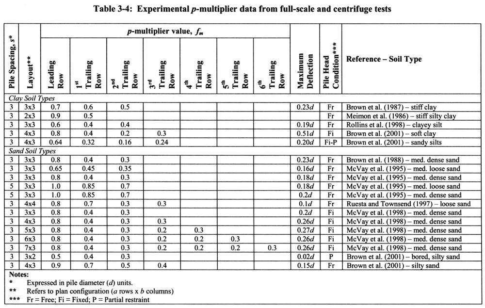
106 86

107 Finally, the issue of structural performance also requires due attention, both in terms of individual pile performance and overall group performance. Ruesta and Townsend (1997) noted the dominance that nonlinear characteristics of prestressed concrete piles had in ultimately assessing p-multipliers, and Brown et al. (2001) stated that modeling of the structural properties of the piles is at least as important as modeling the resistance-deformation [i.e. p-y] behavior of the soil (p. A-6). Not only is the modeling of individual piles in a group important, but also the group as a whole given that the performance of the structural system may overshadow that of the soil system. Brown et al. recognized this quality in conjunction with the 3 x 2 bored pile group test in Taiwan, as although softening of the pile-soil system was observed in connection with the installation process, the relatively high structural stiffness of the group demanded that a focus remain on correctly modeling the structural performance of the pile-soil-cap system. This is a return to the fundamental aspect of soil-structure interaction, whereby behavior is dependent on the relative stiffness of the soil and structure Concluding Comments An appreciable amount of uncertainty is evident in relation to a p-y orientated assessment of lateral behavior for pile groups, arising from the uncertainties associated with the p-y curves themselves, and interrelated issues associated with the determination of group resistance. The pile-soil-pile interaction aspect of the problem certainly plays a significant role in the assessment process, but consideration of other contributing factors and appreciation of the problem as a whole are equally important aspects of the problem. In this respect, Lam et al. (1998) have emphasized the need for equable consideration of the various factors and conditions contributing to group action, pointing out that a p-multiplier of 0.5 may reduce pile-head stiffness by 50%, but this is relatively mild compared with the effect that other issues such as gapping, embedment, and cyclic loading can have on behavior. Altogether, judgment is clearly required and more guidance wanting, particularly in regards to large pile group behavior. 3.6 Design Approaches The importance of lateral stiffness with respect to seismic design is the motivation for the current study, but design for ship impact, wind loading, and wave action are to be also noted from a lateral load design perspective. In terms of designing a laterally loaded pile group, there is a basic need to be able to adequately characterize the behavior of the group taking into account the various issues that have been discussed. In the course of the developments that have taken place towards understanding these issues, a progression of design approaches have naturally emerged. A summary of the prevalent design approaches is provided in Table 3-5. Recent reviews of design methods used in practice (O Neill, Brown, Anderson, El Naggar, Townsend and McVay, 1997; Walsh, Fréchette, Houston and Houston, 2000) indicate variations in the way design approaches are applied, but most revolve around the idea of applying a reduction to the soil system to account for group effects, and then examining the structural integrity of representative piles (or rows) in the group. A general move towards using p-y curves to represent the soil system is suggested, facilitated by the availability of commercial programs such as LPILE (Ensoft, 1999). Emergence of p-y based group programs GROUP (Ensoft, 2004) and FLPIER (McVay et al., 1996) are also influencing the assessment of small pile groups in this way. 87

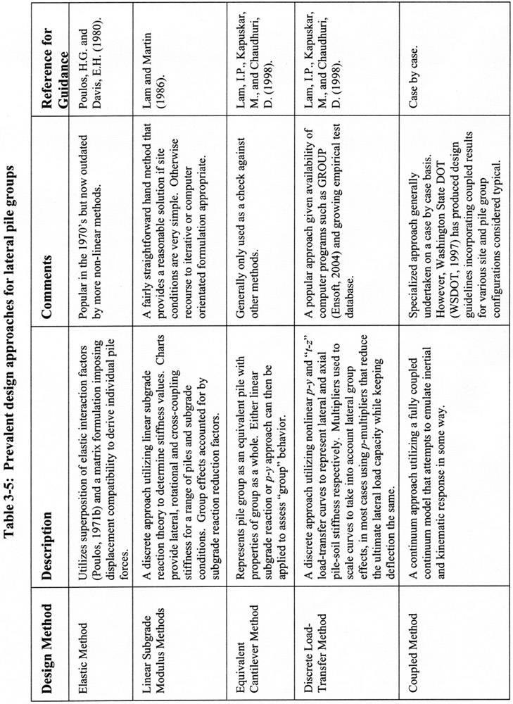
108 88

109 The report by Lam et al. (1998) represents the most up-to-date authoritative reference on lateral pile group behavior, providing some design guidance on many of the issues that have been discussed. A design philosophy urging greater accountability of structural and soil nonlinearity is evident, and the use of p-y curves is the recommended basis for achieving this in the soil case. A key design principle advocated by Lam et al. is an uncoupled approach to account for pile-soil interaction in seismic design. This approach first determines the seismic response of the pile group utilizing linear elastic analysis methods. In this first step importance is given to characterizing a foundation stiffness that seeks to capture the average displacement behavior expected for the seismic conditions at play. If the foundation stiffness is either too high or too low there is a danger of force-displacement incompatibility because of the highly nonlinear nature of soil behavior. This is illustrated in Figure 3-14, which shows a general load-deflection representation of a pile foundation system together with an average design stiffness value. Figure 3-14: General load-displacement relationship illustrating nonlinearity (after Lam et al., 1998) The second step of the design process involves a static nonlinear pushover analysis of the pile group foundation. This determines a realistic force that corresponds with the displacement calculated in the first step, taking into account nonlinearities of the system using discrete load-transfer modeling of the pile group. The second step is then a capacity analysis checking that ductility demand is within the capabilities of the system. In this way a compatible force-displacement regime is determined along with an appropriate stiffness for assessment of the entire system response. Thus the p-y framework is serving a vital role in design and stands to represent the next standard for soil behavior in future pile foundation modeling, underlining the need of appropriate p-y multipliers to assess group effects. 89

110

111 4.1 Introduction SECTION 4 THREE-DIMENSIONAL NUMERICAL MODELING TECHNIQUE The use of mathematical models to idealize physical problems in civil engineering research and design is well-founded. Involved in such an undertaking is the important consideration of establishing whether one-dimensional (1-D), two-dimensional (2-D), or three-dimensional (3-D) numerical means are sufficient to characterize the problem. In the case of the laterally loaded pile group problem where pilesoil-pile interaction takes affect, it is clear from Section 3 that 3-D numerical modeling techniques are necessary from a research perspective to fully appreciate the mechanisms at play. Furthermore, the instance of pile-soil separation and appreciable loading of surficial soils demand both geometric and material nonlinearities be accounted for in the numerical formulation. In previous numerical work the finite element computational framework has been the prevalent 3-D pilesoil modeling tool addressing such needs, as is apparent from the numerical work reviewed in the previous sections. Finite difference modeling techniques have generally not featured in this respect, having been applied instead to 1-D and 2-D problems where finite approximations are used to replace infinitesimal differences that form the components of governing differential equations. For example, the discrete load-transfer approach to pile-soil modeling has typically employed a finite difference solution to the differential equation governing pile behavior, as illustrated in Figure 4-1. Indeed, the term finite difference is often considered synonymous with this type of classical approach, where discretization is in the form of discrete calculation stations that are interrelated via a general finite difference equation, often depicted using finite difference stencils, and unknown variables at each station are solved using matrix algebra. Finite difference approaches are evident in other forms, however, particularly as applied to dynamic problems where they form a basis for direct integration methods that have been developed to solve the dynamic equations of equilibrium. The dynamic equations of equilibrium for a discretized numerical system can be succinctly expressed as where M = mass matrix, U = acceleration vector, M U + CU + KU = R (4.1) C = damping matrix, U = velocity vector, K = stiffness matrix, U = displacement vector, and R = vector of externally applied loads. Application of finite difference expressions for acceleration, velocity and displacement in (4.1) lead to the various direct integration methods, for example the explicit central finite difference method, or the implicit Crank-Nicolson and Houbolt methods. 91

112 P z = axial load Notes: z y h h y m+1 y m = finite difference station h = discretization (increment) length for pile z = depth h y m-1 h Deflected pile h h h h h h Pile characterized by E p I p line element Soil characterized by springs, stiffness = k = (p*h)/y i.e. p p-y curve resistance from lateral reaction k/h 1 y a) Finite difference model 2 d E I 2 dz p y m 2 + y + y m p 2 d y + P 2 dz z 2 d y + ky = 0 2 dz 2 ( Rm 1) + y m 1( 2Rm 2Rm 1 + Px h ) 2 4 ( Rm Rm + Rm 1 2Px h + kmh ) 2 ( 2R 2R + P h ) + y ( R ) m+ 1 where R = E I p p m+ 1 m x m+ 2 Figure 4-1: Finite difference solution scheme for pile-soil interaction problem utilizing the discrete load-transfer approach Contrasting with the classical matrix-orientated finite difference techniques and distinctly temporal finite difference applications is the commercial 3-D explicit finite difference program FLAC 3D (Itasca, 1997). Although drawing on finite difference computation to enable a solution, FLAC 3D also relies on other modeling techniques and concepts to obtain a solution, thus it is best classified as a hybrid modeling technique when considered in the context of finite difference approaches in general. The FLAC 3D formulation is therefore quite unique and represents a computational framework of a very different nature to that of the finite element approach. This demands particular care in the use of FLAC 3D as a modeling tool, weighed down by its relative infancy that affords lack of familiarity and allows only a limited track record from which to assess its performance. m+ 1 = 0 b) Governing differential equation c) General finite difference equation 92

113 The current research adopted FLAC 3D as the 3-D pile-soil modeling tool to undertake numerical studies on the lateral stiffness of pile groups. Given the emphasis of the research on pile groups, and the attendant actions around a pile that this implies, provision of a numerical formulation capable of modeling the pile-soil interface aspect of the problem was considered particularly important. The interface feature in FLAC 3D provided such capabilities, allowing interface action to be implemented in a controlled manner that was considered appropriate to appreciate the mechanics at play. Hence, along with its 3-D formulation and the ability to account for geometric and material nonlinearities, FLAC 3D met the necessary modeling requirements. The current section thus serves to describe FLAC 3D in sufficient detail to address both its capabilities and its uniqueness from a formulation standpoint. 4.2 FLAC 3D Overview In broad terms FLAC 3D (Fast Lagrangian Analysis of Continua in 3 Dimensions) is a three-dimensional, nonlinear, explicit finite difference program that can be used to simulate static and dynamic soil-structure interaction. The basis from which this is achieved is a unique explicit solution scheme that avoids a stiffness-based formulation common in finite element programs. Representing the chief solution vehicle of the explicit solution scheme is the central finite difference expression of Newton s Second Law of Motion: Δt Δt Force v t + = v t + Δt 2 2 Mass where v = velocity, t = time, and Δt = time step. (4.2) Use of the Second Law of Motion follows the dynamic relaxation connotations of FLAC 3D, the idea behind dynamic relaxation being that a dynamic formulation can be used to obtain a static solution based on the fact that the static solution is the steady state part of the transient response of a system (Underwood, 1983). Thus time only serves as a computational device for static problems in FLAC 3D. Constructing the analysis domain using 3-D numerical building blocks (termed zones as opposed to elements used with finite elements), the solution procedure formulates (4.2) at discrete calculation points that locate the vertices of each 3-D zone (termed gridpoints as opposed to nodes used in finite elements). This is undertaken in terms of tetrahedral shapes, whereby the program considers each zone as consisting of pairs of tetrahedron sets, as shown in Figure 4-2. Consideration of each zone in terms of elemental tetrahedra enables the application of an efficient ( fast ) computational algorithm, calling upon the divergence theorem, the principle of virtual work, and linearized velocity fields to apportion gridpoints with an equivalent force that represents the collective actions of forces derived from stressstrain behavior, body and inertial forces, and possible direct point loads applied in relation to boundary conditions. Such forces are collated at each gridpoint from all adjoining tetrahedra for both tetrahedron sets. 93

114 Figure 4-2: Internal tetrahedron sets used in FLAC3D formulation An average of the forces obtained from both tetrahedron sets is used as the value of the gridpoint force to prevent possible directional bias in the solution, brought about by the different geometrical layout of each of the tetrahedron sets. Velocity and displacement are formulated at the gridpoints, while strain and stress tensors are formulated at the centroid of the zone. An illustration of this general analysis concept is illustrated in Figure 4-3. Displacements are calculated at gridpoints by applying central finite difference approximation as follows, u Δt 2 ( t + Δt) = u( t) + v t + Δt (4.3) 94

115 Figure 4-3: General analysis concept in FLAC3D where u = displacement, and in this way the Lagrangian aspect of the formulation is seen to be a matter of course. Both (4.2) and (4.3) are successively applied to each gridpoint of every zone at each time step. The analysis sequence starts with (4.2) and (4.3) applied to obtain velocities and displacements, then velocity-induced strain increments are derived at element centroids, and ensuing stresses are derived via the stress-strain law appropriate to the constitutive model assigned to the zone. Conversion of stresses to gridpoint forces then completes the sequence in readiness for repeating the process for the next time step. This calculation cycle is illustrated in Figure

116 Figure 4-4: Basic calculation cycle in FLAC3D (Itasca, 1997) Hence a physical interpretation of FLAC 3D is that it is depicting a 3-D analysis problem as a system of interconnected but discrete masses and springs that propagate waves numerically using (4.2) as an approximation of the process. In doing so the FLAC 3D formulation is removed from the encapsulated environment evident in finite elements, where the usual displacement-based approach enjoys the equivalency of invoking stationarity of the total potential of the discretized finite element system. Enforcing a system to obey such a well-founded principle serves as an effective theoretical assurance for the finite element approach, but in the FLAC 3D case, existence of such an effective assurance is less apparent. This is where the nature of FLAC 3D deviates from finite elements, shifting the focus instead to the transmission qualities of the system so that the attempt to approximate physical disturbance is made as realistic as possible. Dynamic aspects are therefore of primary concern in the FLAC 3D formulation, irrespective of whether a static or dynamic solution is being pursued. Forming the backbone for this dynamic framework are central finite difference and the spirit of dynamic relaxation. A brief review of these aspects will be undertaken prior to addressing the particulars of the FLAC 3D formulation Central Finite Difference An important consideration when utilizing finite differences is the issue of accuracy. In this way central finite difference performs well as can be demonstrated using Taylor series to obtain the order of accuracy: 96

117 () t ( Δt) d u() t ( Δt) d u() t Δt du u ( t + Δt) = u( t) (4.4) 1! dt 2! 2 3! 3 dt dt () t ( Δt) d u() t ( Δt) d u() t Δt du u ( t Δt) = u( t) + + (4.5) 1! dt 2! 2 3! 3 dt dt Subtracting (4.5) from (4.4) and rearranging, du dt () t u( t + Δt) u( t Δt) O( Δt) 2 = + (4.6) 2Δt which implies that the central finite difference approximation has an error proportional to the square of Δt, and that halving the interval between sample points will reduce the error in the approximation to a quarter of its earlier value. A pictorial of the central finite difference approximation in relation to other finite difference approximations is indicated in Figure 4-5(a) to emphasize the accuracy it affords. Also shown in Figure 4-5(b) is the implication for interrelated variables, as is the case with velocity and displacement (refer Equations 4.2 and 4.3), where the order of accuracy is maintained if the sample points for each variable are offset. u du() t dt Forward finite difference u() t sx Δ x s T x and s T M x T Tx x+ Δx x + Δ x 2 Backward finite difference Central finite difference T 1 M 1 t Δt t t + Δt t O( Δx) 2 accuracy maintained a) Finite difference pictorial b) Accuracy for interrelated variables Dynamic Relaxation Figure 4-5: Central finite difference approximation The spirit of the dynamic relaxation technique is best described by way of demonstration, and the 1-D problem of a bar subject to an axial stress at its free end and fixed at the other will be used for such purposes. This follows Otter, Cassell and Hobbs (1966) who used the problem as an introduction to the dynamic relaxation technique in the mid 1960 s. Details of the problem are given in Figure 4-6, and the central finite difference equations for the governing equations indicated in Figure 4-6(b) are given as follows: 97

118 ( r) ( ) ( u u ) and ( r) E r σ k = k+ 1 k (4.7) Δx σ ( r+ 1) ( r) Kρ 1 ( r 1) ( r) ( u u ) + ( u + u ) ( r) ( r) k σ k 1 ρ + = k k k Δx Δt Δt 2 k (4.8) where the superscript (r) refers to a temporal sample point in computational time, and the subscript k refers to a spatial sample point (i.e., gridpoint). Definitions of terms are given in Figure 4-6. x,u σ = m σ xx σ ε σ xx u K = Eε xx and = ρ + u x t Δ t where xx xx = axial stress = axial strain ρ = mass density u, u, u = axial displacement, velocity andacceleration K = dimensionless damping factor t = fictitious time Δx = 1 ( σ + σ ) = m and u = Figure 4-6: Demonstrative example for dynamic relaxation technique (after Otter et al., 1966) Rearrangement of (4.8) leads to ( r + 1) 1 ( ) ( ) ( r) Δt ( ( r) ( r u = ) ) k K u k σ k σ k K 2 ρδx (4.9) and this provides a starting point for the solution scheme followed by the central finite difference expression for displacement, 98

119 ( r+ 1) k ( r) k ( r+ 1) k u = u + Δt. u (4.10) ( r+1) thus providing the means to calculate σ k from (4.7), whereupon the solution process is repeated for the next time step. A calculation flow as depicted in Figure (c) is therefore effected and this is applied to the gridpoints in succession (spatially) and with each time step (temporally) to seek a solution for the axial displacement, velocity and stress in the bar. The nature of the solution process is typified by the behavior of the free-end of the bar as shown in Figure 4-7. The application of the external stress m disturbs the free-end and this disturbance is propagated numerically through the bar in an iterative fashion using (4.9), (4.10) and (4.7). Removal of kinetic energy is provided by inclusion of a viscous damping mechanism, the physical analogy being a dashpot that consumes a force that is proportional to the velocity of the dashpot. Coupled with enforcement of zero displacement at the fixed end of the bar, a progressive decline in dynamic tendencies is apparent with increasing number of iterations (i.e., computational time) until a static system (and thus solution) prevails. Although a straightforward problem, a number of distinguishing features of the dynamic relaxation technique are evident from the 1-D bar example: (a) use of equations that express behavior in a most physical way, rather than more abstract forms such as derived in finite elements using the principle of virtual displacements; (b) offsetting sample points in both space and time in order to obtain a solution that maintains central finite difference accuracy; and (c) seeking a linear static solution in a progressive, iterative manner, instead of a direct manner such as when inverting a stiffness matrix to solve for unknown displacements. These attributes can be beneficial or detrimental to the cause in hand. In the case of linear static problems they are generally detrimental given the relative efficiency afforded by a displacement-based finite element approach utilizing the more direct stiffness matrix solution technique. A point in favor of dynamic relaxation for this case is less computer memory (storage) requirements, particularly for 3-D problems, however advances in computing power that continue today are serving to downgrade this distinction. It is in the case of a nonlinear static problem where the dynamic relaxation technique stands to provide benefits. The relative simplicity of the computational scheme is obvious, but what is more is the relative ease in which geometric and material nonlinearities can be implemented. This is brought about through the combination of an explicit formulation and use of relatively basic numerical expressions of behavior. However, consideration of a nonlinear system also brings with it the most serious issue of load path dependency, and the associated question of uniqueness of solutions obtained using dynamic relaxation. Load path dependency is an issue because introduction of a damping mechanism dictates the load path experienced by a discretized system when seeking static equilibrium using the dynamic relaxation technique. While a linear elastic system is essentially indifferent to the load path taken, a nonlinear elastic-plastic system will be highly dependent on a load path as this could be the difference between the occurrence of plastic failure or remaining elastic. The onset of plastic failure could conceivably lead to a static equilibrium state different to that obtained had the system remained elastic, or for that matter one that had experienced a different plastic failure regime. Hence one is faced with a possible erroneous static solution state for a nonlinear system when using dynamic relaxation, this being dependent on the performance of the damping mechanism utilized. 99

120 Displacement (m x 10 6 ) Velocity (mm/s) Stress (MPa) Number of Iterations Figure 4-7: Behavior at free-end of 1-D bar during dynamic relaxation solution process (applied axial stress m = 0.7 MPa, K = 0.4) This non-uniqueness aspect of dynamic relaxation invites criticism, and Cundall (1976, 1987) emphasized how deserved this criticism was for the case where velocity proportional damping (i.e. viscous dashpots) was utilized in the dynamic relaxation scheme. This damping mechanism introduces rate-dependent behavior that can only be treated with suspicion. Cundall (1976, 1982, 1987) suggested alternative forms of damping to help overcome some of the difficulties faced when using velocity proportional damping, 100

121 and this work served as a precursor to the approach employed in FLAC 3D*. Thus the FLAC 3D formulation is mindful of the dangers that the dynamic relaxation technique can present, and works to minimize these while still maintaining the thrust of the dynamic relaxation idea to obtain a static solution Formulation Framework Tetrahedral and Gridpoint Actions The independent, or primary, variable in FLAC 3D is velocity, and this is formulated at the gridpoints of 3- D zones that are considered internally as pairs of tetrahedral sets (refer Figure 4-2). A tetrahedron therefore serves as the elemental component for formulation purposes, and the nomenclature associated with this formulation is shown in Figure 4-8. v = v i + v jˆ + v kˆ ˆ = velocity vector at gridpoint 2 z and kˆ 2 x and iˆ y and jˆ 4 iˆ + n ˆj + n f f f nˆ ( f ) ( ) ( ) ( ) = n1 2 3 kˆ = normal vector to face f 3 Face f Surface area = S (f) 1 Notes: 1. i ˆ, ˆj & kˆ = unit vectors in x, y and z directions, respectively. 2. Shaded face in figure corresponds to face number 2 (i.e. f = 2). Figure 4-8: Tetrahedron nomenclature A right-handed Cartesian system is utilized so that vectors (denoted here with an overbar) are expressed in terms of their x, y and z components and respective directions by î, ĵ and kˆ unit vectors. Gridpoint vectors use superscripts to denote the gridpoint number (numbered 1 to 4), and subscripts to denote the Cartesian component (1 = x, 2 = y and 3 = z). The planar faces that define a tetrahedron are denoted by the letter f and numbered such that the face number refers to the number of the gridpoint that does not lie in the plane of the face (refer note 2 in Figure 4-8). The geometry of each face is characterized by a unit vector nˆ normal to the face, in which case bracketed superscripts are used to denote the face number, and subscripts denote the Cartesian components as per the gridpoint vector convention. * Peter Cundall, together with Roger Hart, developed the FLAC 3D and 2-D FLAC programs. 101

122 An application of the divergence theorem serves to provide the means by which volume variables associated with a tetrahedron (i.e., stress and strain) are transformed into discrete variables (i.e. velocities, displacements and forces) associated with the gridpoints of the tetrahedron. This follows by considering velocity as a vector field, represented by a vector point function v ( x, y, z) say, and noting the divergence theorem equality ( n v ) ˆ ds S div v = lim V 0 V wherev = small volume about a point in the vector field, S = surface area of V, ds = differential surface area, v1 v2 v3 and div v = + +. x y z (4.11) By expanding the RHS expression of (4.11), lim V 0 ( nˆ v ) ds v ( n iˆ ) ds v ( nˆ ˆ 1 ˆ 2 j) S V = lim V 0 + lim V 0 S S v 3 V ( nˆ kˆ ) V ds + lim V 0 S V ds (4.12) the following is then apparent, ( nˆ iˆ ) v v1 ds v1n ds 1 S S = lim = lim (4.13) x V 0 V V 0 V 1 and similarly for the y and z components. Reverting to the more compact Einstein indicial notation, a general expression of (4.13) applicable to all components is given by v x where i, j = 1,2,3. i j i j S V 0 V = lim v n ds (4.14) In the case of the planar-faced tetrahedron, the integral in (4.14) becomes an exercise in summation, as follows: Refer Reddick and Miller (1955), pp for engineering proof of equality. 102

123 103 ) ( 4 1 ) ( ) ( ~ f f f j f i S j i S n v ds n v = = (4.15). face surface area of, to face unit vector normal component of, average velocity over face component of where ~ ) ( ) ( ) ( f S f j n f i v f th f j th f i = = = A linear distribution of velocity over each of the tetrahedron faces is assumed in FLAC 3D, so that, by virtue of the numbering system adopted for the gridpoints and faces, an expression for the average velocity over a face is = = 4 1, ) ( 3 1 ~ f h h h f v v (4.16) Substituting (4.16) into (4.15) and performing some algebra, it can be shown that = = = 4 1 ) ( ) ( 4 1 ) ( ) ( ) ( 3 1 ~ h h h j h i f f f j f i S n v S n v (4.17) Hence the general expression given by (4.14) becomes ) ( ) ( h h j h h i j i S n v V x v = = (4.18) whereby the spatial rate of change of velocity throughout the volume of a tetrahedron (i.e., a volume variable) is expressed in terms of gridpoint velocities, unit normal vector components, and the surface area of faces (i.e., discrete variables). It is to be noted that (4.14) refers to an infinitesimal volume and so is an exact relationship, whereas (4.18) is an approximation given the finite volume associated with a tetrahedron. A connection with strain is made by recognizing that velocity is simply the rate of change of displacement per unit time, and from small deformation theory + = i j j i ij x v x v 2 1 ε (4.19) rate tensor. where = strain - ij ε Substituting (4.18) into (4.19) leads to the following expression,

124 h ( h) ( h) ( ) ( v n + v n ) S 4 1 h h i j j i h 1 ε ij = (4.20) 6V = and this constitutes a key equation used in FLAC 3D, quantifying the interrelation between tetrahedral and gridpoint actions Gridpoint Formulation Central to the approach in FLAC 3D is formulation of the problem at the gridpoints. Defining gridpoint behavior are the dynamic equations of equilibrium that can be expressed in general form as follows: σ x ij j + ρ b i dvi dt = 0 (4.21) whereσ ij = stress tensor, ρ = mass density, b = body force acceleration component, and i dvi dt = inertia acceleration component. In order to derive gridpoint expressions for the components of equilibrium, the theorem of virtual work is applied to a tetrahedron using the following expressions for external virtual work rate (E) and internal virtual work rate (I): E = I 4 h= 1 δv h i f = ε ijσ ij V h i + ρb i V δv dv i V ρδv i dvi dv (4.22a) dt δ dv (4.22b) whereδv f h i h i δv δε i ij = i = i = i th th th component of virtual velocity increment at gridpoint component of force at gridpoint h, component of virtual velocity increment within volumev, = incremental virtual strain - rate tensor. h, Beginning with the body force component of the external virtual work rate (represented by the second b term in the expression for E and denoted by E ), the body force is assumed to be constant throughout the tetrahedron, hence both acceleration and mass density terms are brought outside the integrand. In order to h describe δ vi in terms of gridpoint values (i.e. in terms of δ v i ), a local co-ordinate system with an origin at the centroid of the tetrahedron is employed in conjunction with a linear shape function, as described in Figure

125 ' x 3 Origin of local co-ord system = centroid of tetrahedron ' x 2 ' x 1 Tetrahedron N h = c h h ' h ' h ' 0 + c1 x1 + c2 x2 + c3 x3 where N h refers to a shape function with constant coefficients (c 0, c 1, c 2 and c 3 ) applied at gridpoint h to describe the linear variation of virtual velocity within the tetrahedron, viz. 1 0 c + c c c 1 ' 1 1x1 1 ' 2 1x1 + c + c 1 ' 1 2x2 1 ' 2 2x2 + c + c 1 ' 1 3 x3 1 ' 2 3 x3 = 1 = Gridpoint Gridpoint No.2, etc. Figure 4-9: Local co-ordinate system and shape function to describe virtual velocity variation within tetrahedron The body force component of the external work rate is then expressed as follows: E b = ρb = ρb 4 h h i δv V i N h = 1 4 i h= 1 δv h i dv h h ' h ' h, { c0 dv + c1 x1dv + c2 x2dv + c3 x dv } V V V V 3 (4.23) Given that the origin of the local co-ordinate system is at the centroid of the tetrahedron, the latter three terms in the second expression for E b in (4.23) must equal zero, leading to E b 4 = ρ b δv c V (4.24) i h= 1 h h i 0 Consideration of the shape function applied to each gridpoint (refer Figure 4-9) lends itself to matrix representation, wherein Cramer s rule can be used to show that c 0 =1 4, giving the following desired expression for the body force external work rate component: h E b 4 h ρbiv = δ vi (4.25) 4 h= 1 105

126 Considering now the inertial force component of the external virtual work rate (represented by the third i term in the expression for E and denoted by E ), use of the shape function described in Figure 4-9 gives the following: E i 4 = δv ρn h= 1 h i V h dv dt i dv (4.26) An assumption is made that variations of acceleration within the tetrahedron are small enough to permit the acceleration term in (4.26) to be taken outside the integrand, and furthermore the term replaced by gridpoint values of acceleration, as follows: E i = 4 h= 1 δv h i dv dt i h V ρn h dv (4.27) dvi where dt h = acceleration value at gridpoint h. Given that mass density is assumed to be constant throughout the tetrahedron and applying the findings that were evident in progressing from (4.23) to (4.25), the desired expression for the inertial force component of the external work rate is derived: E i 4 h dvi = δvi dt h= 1 h ρv 4 (4.28) The internal virtual work rate expression given by (4.22b) is converted into a gridpoint expression by first noting that from (4.20) the incremental virtual strain-rate tensor ( δ ε ) can be expressed as follows: ij h ( h) ( h) ( ) ( δv n + v n ) S 4 1 h h i j j i V m= 1 δ ε ij = δ (4.29) 6 Substituting (4.29) for δ ε ij in (4.22b) then gives the following, h ( h) ( h) ( ) ( v σ n + δv n ) S 4 1 h h i ij j j ji i 6 h= 1 I = δ σ (4.30) A force vector h T i is now defined as follows, 106

127 T h i ij ( h) ( h) j S = σ n (4.31) and given that the stress tensor is symmetric (i.e. σ = σ ), the desired expression for the internal virtual work rate results: ij ji 4 I 1 h h = i 3 δ v i T (4.32) h= 1 Equating E and I with use of the derived gridpoint expressions (4.25), (4.28) and (4.32) gives the following: h h h h h ρbiv dvi ρv δ vi Ti = δvi fi + (4.33) 4 1 dt h 3 4 h= 1 = Rearranging (4.33) leads to, 4 h= 1 h h h h ρbiv dvi ρv Ti δ vi fi + + = 0 (4.34) dt and, as the virtual velocity increment h δ v i is finite, the expression in the brackets must equal zero, giving f h i h i T = 3 ρbiv + 4 h h dvi m dt (4.35) where m h is a modified gridpoint mass to ensure numerical stability, as is discussed in section The value of (4.35) is that it provides an equation for an equivalent tetrahedral gridpoint force in terms of discrete dynamic equilibrium components, providing the required basis for a discrete formulation at the gridpoints. The formulation is not complete, however, in that consideration must be given to the fact that gridpoints are associated with more than one tetrahedron. Also, it is possible that point loads are applied to gridpoints directly in connection with external or internal boundary conditions, representing an additional force that must be taken into account. The equation used for the gridpoint formulation in FLAC 3D is therefore given as follows, Ti 3 ρbiv + 4 < h> + P < h> i = m < h> dv dt i < h> (4.36) 107

128 where P i refers to a possible point load applied at a gridpoint, and the bracketed superscript notation <h> refers to the sum of contributions of the tetrahedra associated with the gridpoint h. A general summary of the terms is thus dvi m dt ( h) j ( h) T σ n S i ij = = 3 3 ρbiv = body force contribution to gridpoint, 4 P = possible point force applied at gridpoint, and i equivalent force vector at gridpoint from internal stress, = inertial force contribution to gridpoint Solution Vehicle Equation 4.36 provides a statement of the equation of motion at each gridpoint in a form that is suitable for numerical implementation. However, a solution vehicle is still required to march through fictitious time to seek a static solution. This is where the explicit finite difference aspect of FLAC 3D comes into play, utilizing central finite difference to provide an approximation of (4.36) in a temporal sense. Rearranging (4.36) as follows, 1 Ti ρbiv = + < h> m 3 4 < h> < h> dvi < h> + Pi dt (4.37) and given the central finite difference approximation < h> dvi < h> < h> i i dt = v Δt t + v 2 Δt t 2 Δt (4.38) dvi then substituting (4.38) for dt < h> in (4.37) leads to v Δt t + = v 2 Δt Δt t + < h 2 m < Ti ρbiv h> < h> < h> < h> i i + P > i (4.39) which serves as the solution vehicle for marching through fictitious time. It is to be noted that (4.39) maintains central finite difference accuracy by centering about time t, so that the velocities obtained are offset Δ t 2 from the forces, and likewise the ensuing displacements are offset from the velocities Δ t 2 using the following central finite difference approximation: 108

129 < h> < h> < h> Δt ui ( t + Δt) = ui ( t) + Δt. vi t + (4.40) 2 Both (4.39) and (4.40) invoke another measure of approximation in that force, velocity and displacement quantities are determined at different points in fictitious time. This is a relatively insignificant issue, however, given that numerical stability requirements in FLAC 3D restrict Δ t to very small values, resulting in very small errors associated with offsetting solution variables Formulation Aspects A framework providing a means to convey the solution technique in FLAC 3D has been established, but associated with this framework are several aspects requiring attention. These concern numerical stability requirements, performance of the 3-D zones, and damping considerations Numerical Stability The central finite difference approximation applied to the equation of motion in FLAC 3D is an example of an explicit direct integration method, and the conditional stability of such a method is well known. Conditional stability is concerned with a critical time step Δ tc that must be sufficiently small to prevent artificial numerical-made response behavior polluting the system and rendering a computational solution scheme that is unstable. This artificial behavior is seated in the higher modes of vibration of a discrete system, so that knowledge of the period (T) or frequency (ω) of the highest mode is an important consideration in establishing a stability criterion. In FLAC 3D this issue is addressed by drawing on the similarities between the gridpoint framework used to formulate behavior, and a configuration of lumped masses interconnected by springs. A single mass-spring system of such kind is depicted in Figure 4-10(a), together with its dynamic characteristics. The critical time step to be used when calculating the response of this system using the central finite difference technique is also indicated (Bathe, 1996), so that Δt Δtc = T π = 2 m k. By setting Δt = 1 (allowed given the fictitious nature of the computational time) and letting Δ t = Δtc, it follows that 1 2 m = or m = k 2 k 4 (4.41) meaning that the magnitude of the lumped mass and stiffness of the spring for the single mass-spring system must satisfy the relationship given by (4.41) to ensure stability, if a value of unity is adopted for the time step. Considering now the mass-spring system shown in Figure 4-10(b), the infinite extent and symmetry that this demands leads to an equivalent single mass-spring system similar to that shown in Figure 4-10(a), except the spring stiffness is now 4k. Adopting a value of unity for the time step once again, it follows from (4.41) that stability is satisfied in this case if the magnitude of the lumped mass is made equal to or greater than the stiffness of the spring, or m k. 109

130 ω = k m 2π T or T = and Δt = = k m π c 2 m k Figure Mass-spring systems used for numerical stability analysis purposes (after Itasca, 1997) If Δt = 1, the stability criterion m k for the infinite mass-spring system is rigorously correct given that the system has only one mode of vibration. It is also instructive to consider this system as a discretized, one-dimensional elastic bar of infinite extent in the x-direction, whereby the following equivalencies apply (Cundall, 2001): where E = A = cross EA k = and m = ρaδx (4.42) Δx Young' s modulus of - sectional area of ρ = mass density of bar, Δx = discretization length. bar, bar, 110

131 Given that the critical time step for the infinite mass-spring system is Δt c = 2 m 4k = m k (4.43) substituting the expressions for k and m given by (4.42) into (4.43) leads to Δt c = Δx ρ Δx = E C L (4.44) E where C L = = speed of ρ compressional wave in bar. Hence a physical interpretation of the stability criterion is that Δ t must be small enough that the calculation speed does not exceed the transmission speed of the material being deformed. Turning to a FLAC 3D system, there are similarities with the infinite mass-spring system if a tetrahedron gridpoint h is considered as a lumped mass, the magnitude of which is an appropriate mass (m <h> ) as used in (4.39). The network of gridpoints that results from a 3-D model can therefore be considered as a vast array of interconnected lumped masses, the question being the nature of the spring that interconnects them. In FLAC 3D a spring is derived by treating an increment in the equivalent force vector from internal stress as a force-stiffness relationship as follows: dt h i 3 dσ ij = 3 n ( h) j S ( h) = k h ij v h j dt (4.45) where kij h = ij component of stiffness associated with gridpoint h. Diagonal stiffnesses k 11, k 22 and k 33 can therefore be established by setting the velocity v 1, v 2 and v 3 acting at the gridpoint to unity, respectively, so that in general k qq dσ qq ( h) ( h) dt = nq S (4.46) 3 where qq =11, 22 or 33 (where no summation is implied on the repeated index). Given a small increment in fictitious time, it is assumed that the increment in stress Hooke s Law, or specifically dσ qq is governed by dσ = Mdε (4.47) qq 4 where M = constrained modulus = K + G, 3 qq 111

132 so that k qq ε qqmdt ( h) ( h) dt = nq S (4.48) 3 Now from (4.20) h h h h ( ) ( v n + v n ) S 4 1 h q q q q V h= 1 ε qq = (4.49) 6 h q and given that v = 1 at gridpoint q and v = 0 at the other gridpoints, then h q 1 ( h) ( h) nq S ε qq = (4.50) 3V Substituting (4.50) for ε qq in (4.48) leads to ( h) ( h) [ n S ] 2 M k qq = q (4.51) 9V A measure of the stiffness of the spring interconnecting gridpoints is thus obtained from (4.51), and by adopting the stability criterion from the infinite mass-spring system (i.e. m k for Δt = 1), the form of stability criterion used in FLAC 3D is given as follows m h ( h) ( h) [ n S ] h M 2 = k = max i, i = 1,2, 3 9V (4.52) This requires that the greatest diagonal stiffness value is found for each gridpoint and this value is assigned as the magnitude of the mass of the gridpoint in order to satisfy stability requirements. Itasca (1997) note that the infinite mass-spring stability criterion provides an upper-bound value for the gridpoint mass, but it must be noted that use of a diagonal stiffness value deems (4.52) only an approximation from a stability standpoint. Indeed, the value obtained from (4.52) is multiplied by 6.75 in FLAC 3D in recognition of the approximate nature of the approach, effectively applying a factor of safety m = k Δt. of 2.6 on the time step, given that ( ) 2 In physical terms the effective factor of safety applied to the time step ensures that information cannot propagate between gridpoints in one time step. This provides the justification for updating each gridpoint in turn at each time step in the FLAC 3D formulation, given that each gridpoint is effectively isolated from its neighboring gridpoints during this time. An appreciation of the propagation behavior in FLAC 3D can be gained by modeling the 1-D bar problem examined in section and comparing the behavior at the free-end with that obtained using dynamic relaxation. The results are shown in Figure 4-11 and Figure 4-112

133 11, where the FLAC 3D model of the bar was constructed of five unit cube zones to maintain equivalency with the dynamic relaxation model shown in Figure The significantly decreased velocity behavior reflects the more onerous propagation limits imposed in FLAC 3D, requiring more computational steps to obtain the static solution. Displacement (m x 10 6 ) Dynamic Relaxation FLAC3D Number of Iterations Figure 4-11: Comparison of FLAC 3D and dynamic relaxation velocity behavior at free-end of 1-D bar analyzed in section Dynamic Relaxation Vel. (mm/s) Dynamic Relaxation FLAC3D Number of Iterations FLAC 3D Velocity (m/s x 10 6 ) Figure 4-12: Comparison of FLAC 3D and dynamic relaxation displacement behavior at free-end of 1-D bar analyzed in section

134 Damping Scheme Instead of looking to a physical model for energy dissipation, the damping mechanism used in FLAC 3D is a purely mathematical approach based on observed damping behavior. Termed local non-viscous damping, the idea relies on the assumption that a system will oscillate as a result of a disturbance being applied. This is usually a safe assumption, but in the case of flow failure, where a mass may move at a near constant velocity (e.g. ultimate bearing capacity failure), a variation on the idea, termed combined damping, is utilized. Cundall (1987) introduced the idea of local non-viscous damping, and a onedegree-of-freedom (1-DOF) mass and spring system (as per Figure 4-10a) will be used to illustrate the concept. In the absence of energy dissipation, a 1-DOF mass-spring system will oscillate with energy being exchanged between kinetic and strain energy. Introduction of damping serves to add another form of energy interchange, and a schematic illustrating the interplay of system forces is shown in Figure A point to note is the opposing sense of velocity and acceleration variation, but nevertheless an equal area of each quantity, during each quarter-cycle of oscillatory motion. This opposing but equal sense of velocity and acceleration variation is suggestive of a damping force that can be made proportional to force rather than velocity, the latter being the case of viscous damping. F = F + F spring inertia damping F + F = F spring damping inertia F = F + F spring inertia damping F + F = F spring damping inertia Figure 4-13: Oscillating 1-DOF mass-spring system 114

135 A damping force F D is therefore introduced directly into Newton s Second Law of Motion as follows: () t = kx() t FD m x + (4.53) where F D is given by the following: where α = F D () t sgn( v() t ) = α kx (4.54) a damping constant, whose default value is 0.8, and the sgn function is defined as follows: v() t () t v() t + 1, if > 0; sgn( v () t ) = 0, if v = 0; (4.55) 1, if < 0; The effect of this formulation becomes apparent if one considers the oscillation of the 1-DOF mass-spring system when subjected to an initial displacement but no initial velocity. Acceleration (force) and velocity versus time are shown in Figure 4-14, where F(t) = kx(t). By applying (4.54) and (4.55) to each of the intervals indicated on Figure 4-14, the following forms of (4.53) result: Interval 1: F() t + αf() t Interval 2: F() t + αf() t Interval 3: F() t αf() t Interval 4: F() t αf() t + m m where m = and m =. ( 1 α ) ( 1 + α ) ()( t 1 α ) F() t F = mx or x = = (4.56a) m + m ()( t 1 + α ) F() t F = mx or x = = (4.56b) m m ()( t 1 α ) F() t F = mx or x = = (4.56c) m + m ()( t 1 + α ) F() t F = mx or x = = (4.56d) m m 115

136 Interval1: x () + F t = m Interval 1 Interval 2 : x () F t = m Interval 2 Interval 3 : x () + F t = m Interval 3 Interval 4 : x () F t = m Interval 4 Time, t Time, t Figure 4-14: Temporal force and velocity relationship for oscillating 1-DOF mass-spring system The nature of (4.53) and (4.54) guarantees that the damping force acts in the opposite direction to motion (i.e. velocity), just as is the case with viscous damping. However, instead of scaling the damping force to the magnitude of velocity, as is done with viscous damping, the technique simply scales it to the magnitude of the force at play via the α factor. The rightmost expressions in (4.56) and the definitions for m + and m - provide an alternative interpretation in terms of an equivalent mass that the system thinks is present. In terms of kinetic energy, the effect is to extract energy at the peak velocity points, and for one complete cycle the amount extracted (ΔW) is given by ( m m ) v() ΔW = 2 ( t ) (4.57) 2 where is to be noted that the addition of mass at zero velocity has no impact on kinetic energy. Given that this is a simple mass and spring system, the peak kinetic energy is equal to the peak strain energy stored in the spring. The peak kinetic energy (denoted by W) is the average of that produced by both of the equivalent masses i.e. ( m + + m ) v() t 1 W = ( ) 2 (4.58) 4 116

137 This enables a comparison with viscous damping, in that ΔW W 4 = m + ( m m ) = 4α + + m (4.59) and given the following relationship for a viscous damping mechanism ΔW W = 4πξ (4.60) where ξ = the viscous damping ratio, then α ξ = (4.61) π To demonstrate the concept, the case of free vibration was implemented via an Excel spreadsheet utilizing central finite difference approximations of the governing equation of motion. The results are shown in Figure 4-15 and Figure 4-16, where a comparison with the viscous damping solution is also shown. Note that if α = 0.8, then (4.61) gives ξ It is therefore apparent that the local non-viscous damping scheme acts in much the same way as viscous damping, but avoids the danger of velocitydependent damping forces Displacement, x Time, t Alpha = 0.0 Alpha = 0.5 Alpha = 0.8 Figure 4-15: Free vibration behavior of local non-viscous damping mechanism for various α values 117

138 Displacement, x Local damping, constant (Alpha) = 0.8 Viscous, damping ratio (Xi) = Time, t -1.0 Figure 4-16: Comparison of free vibration behavior using local non-viscous damping and viscous damping mechanisms Returning to the FLAC 3D formulation, the local non-viscous damping scheme is easily incorporated by modifying (4.39) to include a damping force as follows: v < h> i Δt t + = v 2 < h> i Δt Δt t + 2 m < h> < h> < h> ( F + F ) i D (4.62) where F F < h> i < h> D Ti ρbiv = = 0.8 F < h> i < h> sgn + P < h> i, < h> ( v ) = gridpoint damping force. i In the combined damping case, where significant uniform motion exists in comparison to the magnitude of oscillations to be damped, use is made of the fact that the derivative of a harmonic force with respect to time is proportional to its harmonic velocity. Thus an additional term is added to the gridpoint damping force expression to accommodate constant velocity (rigid-body) motion equally, as follows: F < h> h> < h> h D i α Fi = 2 < dfi sgn dt sgn < > ( v ) (4.63) 118

139 Zone Performance A zone in FLAC 3D represents the basic numerical building block used to construct a 3-D analysis region to solve a physical problem using mathematical models. This process also applies to a 3-D finite element approach, except continuum brick elements would be used instead of zones. In displacement-based finite element analysis, the performance of such brick elements is concerned with shape functions and their ability to provide a state of strain that is appropriate to the type of deformation experienced by the element. Isoparametric continuum element formulations are typical in this respect, obtaining a strain measure through differentiation of the nodal shape functions so derived, and referring to sampling, or integration points, to establish element values. In terms of the FLAC 3D zone formulation, the means of obtaining a strain measure is different. First of all, rather than using shape functions to describe displacement spatially and then differentiating according to small deformation strain-displacement relations, a spatial derivative of displacement is obtained directly by application of the general integral expression given by (4.14), leading to the tetrahedronspecific formulation given by (4.18). This provides a spatial derivative of displacement (per unit of fictitious time) at the centroid of a tetrahedron, whereupon the small deformation strain-displacement relation given by (4.19) leads to the strain-tensor as given by (4.20), also applying at the centroid. A second difference is in use of the tetrahedron formulation itself, in that zone values of strain and stress (considered to apply at the centroid of the zone) are derived in terms of a weighted average calculation using tetrahedra volumes as the basis, i.e. n Q dvol Zone value = 1 (4.64) n 1 dvol where n = no. of tetrahedra in each zone, Q = stress or strain, dvol = volume of each tetrahedron. Direct comparison of a FLAC 3D zone with an equivalent finite element formulation is therefore obscured numerically, but the linear distribution of velocity over each tetrahedron face, as discussed in section , places a zone in the constant-strain finite element formulation category. Deformation experiments were therefore undertaken to provide a demonstration of the elastic performance of a FLAC 3D zone in comparison with an 8-node 3-D brick element using 2x2x2 integration points, as shown in Figure The analysis program COSMOS/M (Structural Research & Analysis Corp., 1999) was used to undertake the finite element computations. Both a zone and 8-node brick element, shaped in the form of a unit cube and a bar, were tested for stress response by applying appropriate displacements to induce volumetric and shear deformation modes, as detailed in Figure The results are shown in Table 4-1, and are in exact agreement as expected. 119

140 Figure 4-17: Experiments undertaken to compare FLAC 3D and finite element elastic response 120

141 Stress Component Table 4-1: Stress results from FLAC 3D and COSMOS/M comparison Unit Cube Shape (1x1x1) Bar Shape (5x1x1) Deformation Mode Deformation Mode Volumetric Shear Volumetric xy Shear yz Shear A B A B A B A B A B σ xx σ yy σ zz σ xz σ xy σ yz Note: A = FLAC 3D ; B = COSMOS/M A performance aspect of the tetrahedron-based formulation that certainly requires attention is the fact that a tetrahedron does not provide enough flexibility when volumetric restrictions associated with plastic flow conditions are imposed. Severe constraint resulting from the perfect plasticity requirement of zero volume change, leading to overly stiff behavior ( locking ) and thus over-prediction of limit loads, was first explained by Nagtegaal, Parks and Rice (1974). This work used the ratio of total degrees of freedom to total number of incompressibility constraints to characterize the deficiency in volumetric flexibility, noting that a ratio greater than or equal to one was required to avoid locking, whereas a ratio of 3/5 applied to a tetrahedron. In FLAC 3D, this flexibility deficiency is addressed by a procedure termed mixed discretization (Marti and Cundall, 1982). The idea of the mixed discretization procedure is to increase the number of active degrees of freedom for volumetric action by discretizing volumetric strain at the zone level using a weighted average scheme as follows: n ( h) ( h) ε v V h= 1 n ( h) ε = (4.65) v h= 1 where n = number of tetrahedra in a zone, ε V ε = volumetric strain for zone, v ( h) v ( h) V = volumetric strain for each tetrahedron h, = volume of tetrahedron h. While similar in form to (4.64) used to report zone stress and strain values, (4.65) differs in that only the volume component is averaged, and is only invoked when plastic failure occurs. An adjusted strain tensor for each tetrahedron in a zone is then obtained as follows: 121

142 where ε e ( h) ij ( h) ij δ ij ( h) ( h) ε v ε ij = eij + δ ij (4.66) 3 = strain tensor for tetrahedron h, = "original"deviatoric strain tensor for tetrahedron h, = Kronecker delta. Stress components are also adjusted in the same way for consistency. Applying the mixed discretization procedure overcomes locking problems while maintaining appropriate volumetric response, as demonstrated by Marti and Cundall (1982) and as evident in various verification problems provided in the FLAC 3D documentation. It is noted that tetrahedra do not suffer from spurious zero-energy modes associated with the hour-glass modeling problem Interface Behavior Separation and sliding capabilities at the common boundary, or interface of different materials, are provided in FLAC 3D by so-called two-dimensional interface elements. The geometrical configuration of interface elements is indicated in Figure 4-18, comprising triangular elements that cover the faces of each zone that locate the planar boundary that forms the interface of differing materials. A parent face is defined as the face of each zone that the interface is imagined to be wrapped over, the terminology being adopted in light of a physical similarity to shrink-wrap that one could imagine to be stretched over the planar interface surface in order to protect one material from another material that it abuts up against (as per the situation depicted in Figure 4-18). In terms of the interface formulation, the material that the interface is wrapped over is termed the parent material, and each zone in the parent material whose face locates the interface surface is referred to as a parent zone. A neighboring zone of the different material, or target material, is similarly referred to as a target zone. Separation and sliding behavior at the interface is represented by elastic normal and shear springs, respectively, both possessing strength limits. The strength of the shear spring is characterized by Mohr- Coulomb strength parameters c and φ', and a tensile strength is assigned to the normal spring, so that if exceeded, separation occurs (compressive strength being unlimited). The shear and normal springs are considered to exist at interface gridpoints that are indicated in Figure These interface gridpoints always occupy the same position as their parent zone gridpoints, but are attached to the respective target zone gridpoints via the shear and normal springs. The essence of interface action is illustrated in Figure 4-19, where a typical parent and target zone are depicted together with their interface element. As shown, a parent face and target face are defined accordingly. Prior to any movement, referred to as Time Step 0 in Figure 4-19, interface gridpoints and associated parent and target zone gridpoints all occupy the same position. Relative movement between the parent face and target face is then considered to occur as a result of a calculation cycle performed on zone gridpoints, referred to as Time Step 1 in Figure In undergoing the relative movement δ, the shear and normal springs associated with the interface gridpoints are activated, such that each develop a force (referred to here as F int-shear and F int-norm, respectively) corresponding to their respective stiffness multiplied by δ. 122

143 Neighboring zones Material 1 Planar interface between materials Material 2 2-D triangular interface elements that wrap over the face of a parent zone Interface gridpoint A = Interface gridpoint Tribrutary area associated with interface gridpoint A Figure 4-18: 2-D interface elements used in FLAC 3D (after Itasca, 1997) Activation causes F int-shear and F int-norm to be distributed to both the parent zone and target zone gridpoint associated with the interface gridpoint, the distribution being in an equal an opposite fashion to maintain equilibrium. These forces are then additional forces to be accounted for in the gridpoint formulation represented by (4.62). Furthermore, activation also causes the interface gridpoint spring stiffnesses to be added to the parent zone and target zone gridpoint stiffnesses. Distributing to both maintains numerical stability and enforces a reduced relative-movement regime with subsequent time steps given the greater stiffness inherited by the parent zone and target zone gridpoints. The process of relative movement between parent and target faces, that in turn mobilizes interface forces that are then distributed to attached zone gridpoints, is repeated at each time step with total interface forces constantly monitored against the strength limits assigned. 123

144 A Time Step 0: Neighboring zones Target face Note: Target Zone Parent Zone Refer note Interface that is wrapped onto the parent face Parent face Key: Parent face gridpoint Target face gridpoint Interface gridpoint The zones and interface above have been drawn as separated for clarity only. Initially, the target and parent zones abut each other so that the parent and target face gridpoints, and interface gridpoints, all occupy the same position in space. B Time Step 1: Relative movement equal to occurs between parent face and target face, so that the target face can be considered to penetrate into the parent face a distance Note: Interface element remains glued to the parent face, moving with it at all times. Figure 4-19: Essence of interface action in FLAC 3D The magnitude of the stiffnesses assigned to the interface gridpoint springs therefore reflects the type of interface behavior sought: A much greater stiffness compared with that of the zone gridpoint of the associated parent and target zones is akin to a pressure transducer, such that forces are tracked with minimal compliance; whereas a much lesser stiffness compared with that of the zone gridpoint of the associated parent and target zones is akin to a weak discontinuity, such as a clay gouge zone associated with fault movements. In the case of modeling a laterally loaded pile, the interface behavior sought is that akin to a pressure transducer, so that the interface spring stiffnesses must necessarily exceed the zone gridpoint stiffnesses by an appreciable amount. To this end an apparent stiffness of a zone gridpoint in the direction normal to the interface plane is defined as 124

145 where 4 K + G 3 Δz min K & G = bulk and shear moduli of zone, respectively, and Δ z the smallest dimension of the zone. min = (4.67) The apparent stiffness measure accounts for the normal stiffness of a zone as this is a function of its elastic properties and its size. An apparent stiffness value is therefore calculated for the parent and target zones associated with the interface gridpoint, and the maximum value used as a benchmark for characterizing the interface spring stiffness. An interface stiffness that provides at least ten times the maximum apparent stiffness is recommended in FLAC 3D. 4.3 Application to Research The above review indicates the capabilities but uniqueness of FLAC 3D as an analysis tool. In the context of the current research, namely static, monotonic lateral loading of piles, the FLAC 3D formulation provides the necessary modeling requirements to undertake a numerical 3-D assessment of pile-soil interaction. However, a qualification is necessary in terms of the way it is applied to simulate the static, monotonic lateral loading. It is apparent from section and section that FLAC 3D is attempting to approximate the physical disturbance to a soil system brought about by forces imposed on it and manifested as deformation. As with laboratory experiments on soil, such disturbance can be applied via load ( stress control ) or movement ( strain control ). Applying load in FLAC 3D is a matter of applying forces to gridpoints, either through specifying an external stress on a face that is then converted into gridpoint forces, or by specifying external gridpoint forces directly. Applying movement in FLAC 3D is a matter of specifying velocity at a gridpoint, and then stepping through computational time to obtain the specified movement. The amount of stress/force or velocity that is applied to gridpoints is important in that too much can initiate a dynamic shock to the system that is unreasonable from a real physical standpoint. A typical FLAC 3D pile-soil model is shown in Figure 4-20, comprising a pile constructed of elastic zones, surrounding soil constructed of elasticplastic zones, and an interface element wrapped over the soil zone faces that cover the pile-soil interface area. To apply the loading in the direction shown, very small velocity increments were applied to the gridpoints located on the top surface of the pile. These velocity increments were controlled to minimize incremental forces developed in the pile-soil system so as not to pollute the solution with inertial tendencies. Simulation of lateral loading in FLAC 3D was therefore achieved by performing what is essentially a very slow dynamic test. Given the in-built restrictions to ensure numerical stability throughout the system, and the inference to physical propagation of a disturbance that this implies (refer section ), a mathematical model favoring a wave propagation solution approach to the laterally loaded pile problem was therefore realized. 125

146 Ground Level Soil Loading direction Interface between soil and pile Pile (shown detached from soil for clarity) Figure 4-20: Typical FLAC 3D pile-soil model 126