Coarse-Graining via the Mori-Zwanzig Formalism
|
|
|
- Madeline Tyler
- 6 years ago
- Views:
Transcription


1 Coarse-Graining via the Mori-Zwanzig Formalism George Em Karniadakis & Zhen Li Supported by DOE ASCR


2 Mori-Zwanzig can be used to: 1. Derive coarse-grained equations 2. Analyze systems with memory 3. Construct reduced-order models 4. Detect singularities - design meshes 5. Quantify uncertainty
3 Hierarchy of Mathematical & Numerical Models June 23,

4 Hierarchy of Mathematical & Numerical Models June 23,
 ρρρρ(rr) is the conditional probability to find another particle at a distance rr away from the origin.")
5 Radial Distribution Function (RDF) The radial distribution function (or pair correlation function) gg(rr) in a particle-based system describes how density varies as a function of distance from a reference particle. gg rr = 1 ρρρρ NN ii=1,jj ii δδ(rr rr iiii ) ρρρρ(rr) is the conditional probability to find another particle at a distance rr away from the origin. In discrete form: count the number of particles that lie in a spherical shell of radius rr and thickness dddd gg rr = ρρ(rr) ρρ = 1 ρρ NN(rr ± dddd 2 ) /2 4ππrr 2 dddd Number of pairs Volume of the shell
")


6 Radial Distribution Function (RDF) Solid Note: RDF can be measured experimentally using x-ray or neutron-scattering techniques. Liquid Gas Ideal gas: gg(rr) = 1
7 Radial Distribution Function (RDF) Thermodynamic quantities from the computed g(r): Internal Energy EE = 3 2 NNkk BBTT + NN 2 4ππππ 0 rr 2 VV rr gg rr dddd Thermodynamic quantities from the computed g(r): Pressure PP = ρρkk BB TT 2 dddd rr 3 ππρρ2 rr3 0 dddd gg rr dddd Static structure factor: a mathematical description of how a material scatters incident radiation: SS kk = 1 + 4ππππ rr 2 gg rr 0 sin kkkk kkkk dddd
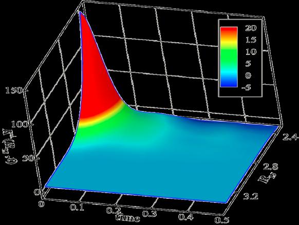
 Long time: CC tt tt 3/2 (Bulk), CC tt tt 5/2 or tt 7/2 (confinement) CC tt = 3kk BBTT MM exp γγγγ MM + 2kk BBTT ρρρρ 4ππ(DD + νν)tt 3 2 Algebraic tail of the VACF:")
8 Velocity Autocorrelation Function (VACF) Definition: CC tt = VV tt VV(0) which reveals the underlying nature of the dynamical processes operating in a molecular system. Short time: CC tt exp( γγγγ/mm) Long time: CC tt tt 3/2 (Bulk), CC tt tt 5/2 or tt 7/2 (confinement) CC tt = 3kk BBTT MM exp γγγγ MM + 2kk BBTT ρρρρ 4ππ(DD + νν)tt 3 2 Algebraic tail of the VACF: Diffusion constant is the integral of VACF: DD = dddd VV ττ VV(0)
9 Fluctuation-Dissipation Theorem (FDT) The FDT quantifies the relation between the fluctuations in a system at thermal equilibrium and the response of the system to applied perturbations. Let xx tt be an observable of a dynamical system with Hamiltonian HH 0 (xx) subject to thermal fluctuations. xx tt fluctuates around its mean value xx 0 and the power spectrum of fluctuations is denoted by SS xx ωω. Consider a time-dependent field ff(tt) that alters the Hamiltonian to HH xx = HH 0 xx + ff t xx. The response of xx(tt) to ff(tt) is characterized by the linear response function χχ tt of the system xx(tt) = xx 0 + tt ff ττ χχ tt ττ dddd The fluctuation-dissipation theorem relates the power spectrum of xx to the imaginary part of the Fourier transform χχ ωω of the susceptibility χχ(tt) SS xx ωω = 2kk BBTT ωω Im χχ(ωω) The left-hand side describes fluctuations in xx, the right-hand side relates to the energy dissipated by the system when pumped by an oscillatory field ff tt = FFsin(ωωωω + φφ). For a particle-based stochastic system, a canonical ensemble is expected only if the FDT is satisfied. Otherwise, the system cannot reach a thermal equilibrium at the designed temperature. R. Kubo, The fluctuation-dissipation theorem
10 DPD : Pairwise Interactions Forces exerted by particle J on particle I: Fluctuation-dissipation relation: σ 2 = 2 γ κ Β Τ ω D = [ ω R ] 2 Conservative fluid / system dependent Dissipative frictional force, represents viscous resistance within the fluid accounts for energy loss j r ij r i i Random stochastic part, makes up for lost degrees of freedom eliminated after the coarse-graining r j 10
11 Outline 1. Introduction Bottom-up coarse-graining 2. Foundation: Coarse-Graining Introduction of the Mori-Zwanzig formalism. Markovian model Non-Markovian model 3. Construction of coarse-grained model directly from MD simulation Static properties Dynamics properties 4. Summary
12 Different coarse graining strategies Reverse coarse graining procedure An initial guess of the CG force fields is posed at the beginning and many free parameters in a coarse-grained model are left undetermined. Subsequently, an (iterative) inverse optimization is carried out to get the optimal free parameters so that target properties are obtained. Target properties Optimization Note: No guarantee of correct properties beyond targets. Forward coarse graining procedure ( No prior targets assigned ) The CG force fields are constructed directly from MD trajectories via the Mori-Zwanzig projection. This procedure may require additional assumptions for simplification of formulation; in principle, there are no free parameters to be specified.
13 Outline 2. Foundation: Coarse-Graining Introduction of the Mori-Zwanzig formalism Markovian model Non-Markovian model

 C")

14 Coarse-Graining CG: remove irrelevant degrees of freedom from a system Microscopic system All-atom model MD Dipalmitoylphosphatidylcholine (DOPC) C 40 H 80 NO 8 P C G Irrelevant variables are eliminated Mesoscopic system Coarse-grained model DPD
15
16 Elimination of degrees of freedom from a system Dimension Reduction leads to memory effect and noise term.
17 Dissipative Particle Dynamics (DPD) 1. Mori-Zwanzig formulation 2. Direct construction of DPD from MD
18 Equation of Coarse-Grained System CG (slower) Variables Atomistic (fast) variables
19 Mori-Zwanzig Formalism (Zwanzig, Nonequilibrium Statistical Mechanics, 2001) Consider a n-dimensional system of ordinary differential equations
20 Mori-Zwanzig Formalism (Zwanzig, Nonequilibrium Statistical Mechanics, 2001) Consider P + Q = II, we have eetttt xx jj = ee tttt LLxx jj = ee tttt P + Q LLxx jj = ee tttt PLLxx jj + ee LLLL QLLxx jj Using Dyson s formula (Duhamel s principle) tt ee tttt = ee ttqll + ee tt ττ LL PLLee ττqll dddd 0 We obtain the Mori-Zwanzig equation tt eetttt xx jj = ee tttt PLLxx jj + ee tt ττ LL PLLee τττττ QLLxx jj dddd + ee ttqll QLLxx jj 0 This equation is exact and is an alternative way of writing the original system of ODEs.
21 Mori-Zwanzig Formalism (Zwanzig, Nonequilibrium Statistical Mechanics, 2001) If the coordinates and momenta of the center of mass of the coarse-grained particles are defined as CG variable to be resolved RR II = 1 mm MM I,ii rr I,ii II I,ii PP II = I,ii pp I,ii MM II = Define P and Q as projection operators for a phase variable AA P( ) = AA TT Q = II P AAAATT 1 ββ JJ 0 tt dddd δδffii QQ tt ss δδff JJ QQ 0 TT PP JJ MM JJ + δδff II QQ (tt) I,ii mm I,ii Given AA the coarse-grained momentum, we identify ee ttttt QLLAA as the random force δδff QQ (tt). Finally, we have the equation of motion for coarse-grained particles dd ddtt PP II = 1 lnωω RR ββ RR II QBB Details see Kinjo, et. al., PRE Lei, et. al., PRE, Hijon, et. al., Farad. Discuss., BB PBB AA

22 Mori-Zwanzig Formalism (Zwanzig, Nonequilibrium Statistical Mechanics, 2001) Consider an atomistic system consisting of N atoms, which are grouped into K clusters, and N C atoms in each cluster. The Hamiltonian of the atomistic system is: H K N C 2 pµ, i 1 = + 2m 2 µ = 1 i= 1 µ, i µν, i, j i V µ i, ν j Atomistic Model Our interest is on the molecular or CG level : M P R = µ µ, i µ, i = µ µ, i µ, i = 1 p m m r µ µ, i µ, i M µ µ, i The equation of motion for CG particles can be written as: Details see Kinjo, et. al., PRE Lei, et. al., PRE, Hijon, et. al., Farad. Discuss., 2010.
23 Bottom-up coarse-grained model: δδff QQ IIII QQ δδff TT IIII JJ KK = 0


24 Evaluation of coarse-grained interactions: First term: Conservative Force: Second term: Dissipative Force: δδff QQ IIII QQ δδff TT IIII JJ KK = 0
25 Coarse-Grained Modeling - Summary The equation of motion (EOM) of coarse-grained particles resulting from the Mori-Zwanzig projection is given by: Conservative force Dissipative force Random force Approximations for computing the coarse-grained forces: Pairwise decomposable: total force consists of pairwise forces FF II II JJ FF IIII Negligible many-body correlations: δδff QQ QQ IIII δδff TT IIKK JJ KK = 0 Then, the above EOM can be written into its pairwise form: where FF IIII is the instantaneous force whose ensemble average FF IIII as the conservative force, the memory kernel KK IIII tt = ββ δδff QQ IIII (tt) which satisfies the second fluctuation-dissipation theorem (FDT). is taken QQ (0) TT, δδff IIJJ
26 General Equation of Coarse-Grained particles Harmonic chain Ensemble average Dissipative force Random force
27 Question Coupled term General Coarse-grained Equation? Mesoscopic Dynamics
28 Langevin Equation Markovian Approximation

29 DPD from Coarse-Grained Equation
30 (Cont'd) Markovian approximation Transverse term Standard DPD

31 This image cannot currently be displayed.
32 MD to DPD Microscopic system (Molecular Dynamics) What is Preserved? What is Lost? Conservative force Dissipative force Random force Mesoscopic system (DPD)
33 Conservative potential (force) term

34
35 Dissipative force term Rg = 0.95 Rg =
36 (Cont'd)
37 Question Microscopic System Fluid Structure? Mesoscopic System

38 Static properties
39 Question Microscopic System Dynamic Properties? Mesoscopic System
40 Dynamic Properties
41 Computing CG interactions Pairwise Potential Memory Kernel K(t) Let the difference of the instantaneous force from the mean force be the fluctuating force, e.g., δδff IIII tt = FF IIII tt FF IIII. By multiplying VV TT IIII 0 on both sides of above equation
42 Markovian DPD model If the typical time scales of random force and momentum are well separated, the Markovian assumption can be applied, where the time correlation of random force is approximated by the δ-function: KK tt γγγγ(t), where γγ = 0 KK tt dddd As a result, the EOM of DPD particles is given by:
43 Non-Markovian DPD model Without the Markovian approximation, we have to preserve the temporal memory of each pair in the NM-DPD model To avoid prohibitive computational cost, we assume that the memory is finite, e.g., history length NNΔtt. Then, the EOM of NM-DPD particles is given by:
 δδff RR IIII (0) TT = 2kk BB TTγγ IIII δδ(tt) Non-Markovian DPD Model The FDT requires δδff QQ IIII (tt) δδff QQ IIII (0) TT = kk BB TTKK IIII (tt), Then, the random force is colored")
44 Fluctuation-Dissipation Theorem Markovian DPD Model the time correlation of random force is approximated by the δ- function Then, the random force is white noise, with variance given by δδff QQ IIII (tt) δδff RR IIII (0) TT = 2kk BB TTγγ IIII δδ(tt) Non-Markovian DPD Model The FDT requires δδff QQ IIII (tt) δδff QQ IIII (0) TT = kk BB TTKK IIII (tt), Then, the random force is colored noise.
45 Colored noise generator 1 (Fourier transform): Consider discrete time steps tt nn = nn δδδδ, nn > 0. We define RR nn = RR tt nn δδδδ tt nn, θθ nn = θθ(tt nn ) KK(tt nn ) In the discrete form, the second FDT is RR nn RR mm TT = kk BB TT θθ nn mm Let 0 nn NN, we can use a periodic extension, which does not affect the values within the first NN steps. We write θθ nn as N θn= αα s s + n s= N In this case, the Fourier transform is reduced to a discrete Fourier transform. N ˆ θn = θne n= N ikn2 π / N Define αα kk = θθ 0.5 kk, the inverse Fourier transform is given by N 1 iks2 π / N α ˆ s = αke 2N + 1 n= N Let WW nn be identically distributed random variables, we generate the colored N noise by Rn= kt B α swn+ s s= N
46 Colored noise generator 1 (Fourier transform): Test Case ) ff(tt = RR nn RR mm LL time = 0.39 Π = 0.78 = 2LL time
47 Colored noise generator 2 (Optimization): Let WW nn be identically distributed random variables, the random force RR nn is given by 0 R = kt W n B α s n+ s s= N where αα nn are undetermined coefficients. Then, the correlation of the random force can be computed by RR = kt 0 0 n m B s t n+ s m t s= Nt= N 0 To satisfy the second FDT, we need ααδ = kt αα = kt f RR B s n m+ s B n m s= N = ktθ n m B n m Numerical optimization techniques can be used to obtain a set of coefficients αα nn by minimization of LL 2 ff nn mm θθ nn mm.

48 Colored noise generator 2 (Optimization): Test Case ) ff(tt = RR nn RR mm LL time = 0.39 Smooth VACF No periodicity
49 Outline 3. Construction of coarse-grained model directly from MD simulation Static properties Dynamics properties


50 Microscopic system to be reproduced Consider a well-defined atomistic system consisting of N atoms which are grouped into K clusters, and N c atoms in each cluster. Microscopic system: WCA Potential + FENE Potential NVT ensemble with Nose-Hoover thermostat. M P R µ µ, i µ, i = = µ µ, i µ, i = µ µ, i µ, i M µ µ, i µ, i 1 p m m L= ( r R ) ( p P ) r µ, i µ µ, i µ

51 Microscopic system to be reproduced Two test systems:
 v = v v e e ij ij ij ij ij 1 eij = vij / vij 3.")
52 Coarse-Grained force field Definition of the directions for pairwise interactions between neighboring clusters: 1. Parallel direction: r = r r e ij i j = r / r ij ij ij 2. Perpendicular direction #1: v = v v ij i j ( ) v = v v e e ij ij ij ij ij 1 eij = vij / vij 3. Perpendicular direction #2: e = e e 2 1 ij ij ij


53 Coarse-Grained force field CG force field obtained directly from MD simulations No freedom to adjust parameters


54 Comparison Atomistic Model Coarse-Grained Model Coarse Graining Hard Potential CG Potential MD DPD


55 Comparison: Static Properties Radial distribution function (RDF) and Pressure (P) of MD, DPD and NM-DPD systems: Observation: Including non-markovian memory in the DPD system does not change its performance on reproducing RDF. Reason: RDF of a DPD system is only determined by the conservative force, and the changes of non-conservative force do not affect RDF, even if the non-markovian memory is introduced in the simulations.
56 Comparison: Dynamic Properties (ρ=0.4) Performance of Markovian DPD model (DPD) and non-markovian DPD model (NM-DPD) in reproducing the MD systems on the velocity autocorrelation function (VACF): MD: DD = 0.119, νν = DPD: DD = 0.120, νν = Both Markovian model and Non-Mavkovian model can reproduce the original MD system well. Including memory does not change the results significantly, which indicates the Markovian assumption can be applied safely.
57 Comparison: Dynamic Properties (ρ=0.4) The curve of Velocity Auto-Correlation Function (VACF) contains dynamic properties of the system 3kT B γ t VACF( t) = exp M M 2kT B 1 + ρm π D ν t [ 4 ( + ) ] 3/2 MM is the mass of a spherical particle. γγ is the Stokes viscous drag coefficient. Short time: VVVVVVVV ~ exp( tt/ττ pp ) Long time: VVVVVVVV ~ tt 3/2 Timescales: ττ pp = MM/γγ Quantities MD DPD (error) Pressure (+1.0%) Diffusivity (Integral of VACF) (+0.8%) Viscosity (-1.1%) Schmidt number (-2.0%) Stokes-Einstein radius (+0.3%)
58 Discussion: Many-Body effect (ρ=0.4)
59 Discussion: Many-Body effect (ρ=0.4) NN cc = 21 NN cc = 31 Quantities MD DPD (error) Pressure (-2.0%) Diffusivity (Integral of VACF) (-1.6%) Viscosity (+3.1%) Schmidt number (+4.8%) Stokes-Einstein radius (-1.4%) Quantities MD DPD (error) Pressure (-3.8%) Diffusivity (Integral of VACF) (-10.0%) Viscosity (+11.1%) Schmidt number (-23.5%) Stokes-Einstein radius (0.0%)
60 Forward CG strategy vs Reverse CG strategy Suppose that the pairwise potential is given, the optimization process only considers the dynamics properties. Set target properties (case NN CC = 21 at ρρ = 0.4) DD, νν MMMM = 0.061, The dissipative force is in the form of FF DD IIII RR = γγ 1 RR/RR ss cccccc VV IIII ee IIII ee IIII Reverse CG strategy optimizes a parameter set γγ, ss to obtain targets. Technically, we employ generalized polynomial chaos (gpc) to construct a surrogate model for DPD systems using a linear combination of a set of special basis functions defined in the parameter space. γγ, ss = γγ, ss + δδ γγ, δδ ss dddddddd ξξ 1, ξξ 2 γγ, ss = 100, 3.0 δδ γγ, δδ ss = 50, 1.0 ξξ 1 and ξξ 2 are i.i.d. uniform random variables distributed on [-1,1].
![Forward CG strategy vs Reverse CG strategy Define error function: Δ = νν νν ref νν ref + DD DD ref DD ref Optimal choice: Δ min = 0.063 γγ, ss = [144.0, 2.42] yields DD, νν = [0.064, 1.](/docs-images/79/80191773/images/61-2.jpg "433] When reverse CG strategy is employed to construct CG models, even if the target properties are achieved, one should not expect that other behavior besides the targets can be correct")
61 Forward CG strategy vs Reverse CG strategy Define error function: Δ = νν νν ref νν ref + DD DD ref DD ref Optimal choice: Δ min = γγ, ss = [144.0, 2.42] yields DD, νν = [0.064, 1.433] When reverse CG strategy is employed to construct CG models, even if the target properties are achieved, one should not expect that other behavior besides the targets can be correct automatically. Z. Li, X. Bian, X. Yang and G.E. Karniadakis, J. Chem. Phys., 2016 (under review).
 Performance of Markovian DPD model (DPD) and non-markovian DPD model (NM-DPD) in reproducing the MD systems on the velocity autocorrelation function (VACF): NM-DPD can reproduce correct short-time")
62 Comparison: Dynamic Properties (ρ=0.7) Performance of Markovian DPD model (DPD) and non-markovian DPD model (NM-DPD) in reproducing the MD systems on the velocity autocorrelation function (VACF): NM-DPD can reproduce correct short-time properties that are related to how the system responds to high-frequency disturbances, which cannot be captured by the Markovian-based DPD model. However, computation of the time convolution is expensive.
63 Markovian system generating non-markovian dynamics Consider a Markovian system described by the stochastic differential equation Ceriotti et al., J. Chem. Theory Comput. (2010).

64 Markovian system generating non-markovian dynamics which corresponds to a non-markovian dynamics. If the memory kernel can be approximated by an arbitrary combination of complex exponentials in the form of then, the non-markovian dynamics can be approximated by the Markovian system whose momentum is coupled to auxiliary variables Ceriotti et al., J. Chem. Theory Comput. (2010).
65 Markovian system generating non-markovian dynamics Relation between the memory kernel KK(tt) and the matrix AA AA pppp Suppose we have the matrix AA = AA pppp = AA ssss AA ssss 0 cc 1 cc 2 cc 1 aa bb cc 2 bb 0, where AA ssss = aa bb bb 0 we can do the eigen-decomposition of AA ssss AA ssss = QQQQQQ 1 = aa aa2 4bb 2 aa+ aa2 4bb 2 2bb 2bb 1 1 aa aa 2 4bb where 1 2 aa±1 2 aa2 4bb 2 are the eigenvalues of the matrix AA ssss. Then the kernel function KK(tt) can be computed by 0 aa+ aa 2 4bb 2 2 bb 1 aa 2 4bb aa 2 aa 2 4bb 2 bb 1 aa aa 2 4bb aa 2 4bb 2 KK tt = AA pppp exp ttaa ssss AA ssss = AA pppp QQQQQQQQ tttt QQ 1 AA ssss = = exp aa 2 tt cc cc 2 2 cos 4bb 2 aa 2 tt + cc 2 cc1 2 aa 2 4bb2 aa 2 4bb 2 aa 2sin 2 tt Given a memory kernel KK tt, which is fitted by KK tt = pp exp qqqq cos(rrrr + ss) Then, we have aa = 2qq, bb = rr 2 + qq 2, cc 1 = qq cos ss rrrr sin(ss), cc 2 2qq 2 = qq 2 cos ss +rrrr 2qq sin(ss)
 ii=1 Parallel component is fitted by 4 terms Perpendicular component is fitted by 2 terms Based on the fitting function, the coupling matrices can be constructed: To satisfy the")
66 Markovian system generating non-markovian dynamics The computed memory kernel can be fitted by a linear combination of many exponentially nn damped oscillations ff tt = Λ ii exp tt/ττ ii cos(ωω ii tt + φφ ii ) ii=1 Parallel component is fitted by 4 terms Perpendicular component is fitted by 2 terms Based on the fitting function, the coupling matrices can be constructed: To satisfy the fluctuation-dissipation theorem, the matrix BB is determined by BBBB TT = kk BB TT(AA ssss + AA TT ssss )
67 Markovian system generating non-markovian dynamics CCCCCCCCCCCCCCCCCCCCCCCCCC cccccccc NNNN DDDDDD CCCCCCCCCCCCCCCCCCCCCCCCCC cccccccc DDDDDD AAAAAA = 8.3ss 0.42ss = 19.8 Z. Li, H.S. Lee, E. Darve and G.E. Karniadakis, 2016 (to be submitted).

68
69 Outline 4. Summary
70 Summary We demonstrated that coarse-grained models can be constructed directly from microscopic dynamics based on the Mori-Zwanzig (MZ) formalism. Given correct CG force field, CG system can reproduce its underlying MD system for both static and dynamic properties. The Markovian assumption works well for the system with clear timescale separation; the NM-DPD model has little improvement on the VACF compared with Markovian DPD model. When the timescales of a system are not fully separated, the NM-DPD can reproduce correct short-time properties that are related to how the system responds to high-frequency disturbances, which cannot be captured by the Markovian-based DPD model. A Markovian system with auxiliary variables coupled to momentum can be employed to generate accurate non-markvoian dynamics with much less computational cost. Z. Li, et al, Soft Matter, 10, 8659, Z. Li, et al. J. Chem. Phys., 2015, 143:
71 References R. Zwanzig, Memory Effects in Irreversible Thermodynamics. Phys. Rev., (4): p H. Mori, Transport Collective Motion and Brownian Motion. Prog. Theor. Phys., (3): P. Espa nol, Dissipative particle dynamics for a harmonic chain: A first-principles derivation. Phys. Rev. E, (2): A.J. Chorin, O.H. Hald, and R. Kupferman, Optimal prediction and the Mori- Zwanzig representation of irreversible processes. PNAS, (7): R. Zwanzig, Nonequilibrium Statistical Mechanics. New York: Oxford University Press T. Kinjo and S.A. Hyodo, Equation of motion for coarse-grained simulation based on microscopic description. Phys. Rev. E, (5): C. Hijon, P. Espa nol, E. Vanden-Eijnden and R. Delgado-Buscalioni, Mori-Zwanzig formalism as a practicalcomputationaltool. Faraday Discuss : H. Lei, B. Caswell and G.E. Karniadakis, Direct construction of mesoscopic models from microscopic simulations. Phys. Rev. E, (2):
: 1170-1180. W. E, Principles of Multiscale Modeling. New York: Cambridge University Press. 2011. Y. Yoshimoto, et al.")
72 References X.T. Li, A coarse-grained molecular dynamics model for crystalline solids. Int. J. Numer. Meth. Eng (8-9): M. Ceriotti, G. Bussi, and M. Parrinello, Colored-Noise Thermostats a la Carte. J. Chem. Theory Comput (4): W. E, Principles of Multiscale Modeling. New York: Cambridge University Press Y. Yoshimoto, et al., Bottom-up construction of interaction models of non-markovian dissipative particle dynamics. Phys. Rev. E, (4): Z. Li, X. Bian, B. Caswell and G.E. Karniadakis, Construction of dissipative particle dynamics models for complex fluids via the Mori-Zwanzig formulation. Soft Matter, (43): M. Chen, X.T. Li, and C. Liu, Computation of the memory functions in the generalized Langevin models for collective dynamics of macromolecules. J. Chem. Phys (6): Z. Li, X. Bian, X.T. Li and G.E. Karniadakis, Incorporation of memory effects in coarse-grained modeling via the Mori-Zwanzig formalism. J. Chem. Phys (24):
APMA 2811T. By Zhen Li. Today s topic: Lecture 2: Theoretical foundation and parameterization. Sep. 15, 2016
 Today s topic: APMA 2811T Dissipative Particle Dynamics Instructor: Professor George Karniadakis Location: 170 Hope Street, Room 118 Time: Thursday 12:00pm 2:00pm Dissipative Particle Dynamics: Foundation,
4. The Green Kubo Relations
 4. The Green Kubo Relations 4.1 The Langevin Equation In 1828 the botanist Robert Brown observed the motion of pollen grains suspended in a fluid. Although the system was allowed to come to equilibrium,
Angular Momentum, Electromagnetic Waves
 Angular Momentum, Electromagnetic Waves Lecture33: Electromagnetic Theory Professor D. K. Ghosh, Physics Department, I.I.T., Bombay As before, we keep in view the four Maxwell s equations for all our discussions.
Review for Exam Hyunse Yoon, Ph.D. Adjunct Assistant Professor Department of Mechanical Engineering, University of Iowa
 Review for Exam2 11. 13. 2015 Hyunse Yoon, Ph.D. Adjunct Assistant Professor Department of Mechanical Engineering, University of Iowa Assistant Research Scientist IIHR-Hydroscience & Engineering, University
Review for Exam Hyunse Yoon, Ph.D. Assistant Research Scientist IIHR-Hydroscience & Engineering University of Iowa
 57:020 Fluids Mechanics Fall2013 1 Review for Exam3 12. 11. 2013 Hyunse Yoon, Ph.D. Assistant Research Scientist IIHR-Hydroscience & Engineering University of Iowa 57:020 Fluids Mechanics Fall2013 2 Chapter
Review of Last Class 1
 Review of Last Class 1 X-Ray diffraction of crystals: the Bragg formulation Condition of diffraction peak: 2dd sin θθ = nnλλ Review of Last Class 2 X-Ray diffraction of crystals: the Von Laue formulation
(1) Introduction: a new basis set
 Introduction: a new basis set") () Introduction: a new basis set In scattering, we are solving the S eq. for arbitrary VV in integral form We look for solutions to unbound states: certain boundary conditions (EE > 0, plane and spherical
() Introduction: a new basis set In scattering, we are solving the S eq. for arbitrary VV in integral form We look for solutions to unbound states: certain boundary conditions (EE > 0, plane and spherical
Gradient expansion formalism for generic spin torques
 Gradient expansion formalism for generic spin torques Atsuo Shitade RIKEN Center for Emergent Matter Science Atsuo Shitade, arxiv:1708.03424. Outline 1. Spintronics a. Magnetoresistance and spin torques
CHAPTER 5 Wave Properties of Matter and Quantum Mechanics I
 CHAPTER 5 Wave Properties of Matter and Quantum Mechanics I 1 5.1 X-Ray Scattering 5.2 De Broglie Waves 5.3 Electron Scattering 5.4 Wave Motion 5.5 Waves or Particles 5.6 Uncertainty Principle Topics 5.7
Information loss and entropy production during dissipative processes in a macroscopic system kicked out of the equilibrium
 Information loss and entropy production during dissipative processes in a macroscopic system kicked out of the equilibrium Peter Burgholzer 1, 2 1 Christian Doppler Laboratory for Photoacoustic Imaging
Review for Exam Hyunse Yoon, Ph.D. Adjunct Assistant Professor Department of Mechanical Engineering, University of Iowa
 Review for Exam3 12. 9. 2015 Hyunse Yoon, Ph.D. Adjunct Assistant Professor Department of Mechanical Engineering, University of Iowa Assistant Research Scientist IIHR-Hydroscience & Engineering, University
Charge carrier density in metals and semiconductors
 Charge carrier density in metals and semiconductors 1. Introduction The Hall Effect Particles must overlap for the permutation symmetry to be relevant. We saw examples of this in the exchange energy in
Mathematics Ext 2. HSC 2014 Solutions. Suite 403, 410 Elizabeth St, Surry Hills NSW 2010 keystoneeducation.com.
 Mathematics Ext HSC 4 Solutions Suite 43, 4 Elizabeth St, Surry Hills NSW info@keystoneeducation.com.au keystoneeducation.com.au Mathematics Extension : HSC 4 Solutions Contents Multiple Choice... 3 Question...
MD Thermodynamics. Lecture 12 3/26/18. Harvard SEAS AP 275 Atomistic Modeling of Materials Boris Kozinsky
 MD Thermodynamics Lecture 1 3/6/18 1 Molecular dynamics The force depends on positions only (not velocities) Total energy is conserved (micro canonical evolution) Newton s equations of motion (second order
The Bose Einstein quantum statistics
 Page 1 The Bose Einstein quantum statistics 1. Introduction Quantized lattice vibrations Thermal lattice vibrations in a solid are sorted in classical mechanics in normal modes, special oscillation patterns
Mutual diffusion of binary liquid mixtures containing methanol, ethanol, acetone, benzene, cyclohexane, toluene and carbon tetrachloride
 - 1 - PLMMP 2016, Kyiv Mutual diffusion of binary liquid mixtures containing methanol, ethanol, acetone, benzene, cyclohexane, toluene and carbon tetrachloride Jadran Vrabec Tatjana Janzen, Gabriela Guevara-Carrión,
Module 7 (Lecture 25) RETAINING WALLS
 RETAINING WALLS") Module 7 (Lecture 25) RETAINING WALLS Topics Check for Bearing Capacity Failure Example Factor of Safety Against Overturning Factor of Safety Against Sliding Factor of Safety Against Bearing Capacity Failure
Module 7 (Lecture 25) RETAINING WALLS Topics Check for Bearing Capacity Failure Example Factor of Safety Against Overturning Factor of Safety Against Sliding Factor of Safety Against Bearing Capacity Failure
ECE 6540, Lecture 06 Sufficient Statistics & Complete Statistics Variations
 ECE 6540, Lecture 06 Sufficient Statistics & Complete Statistics Variations Last Time Minimum Variance Unbiased Estimators Sufficient Statistics Proving t = T(x) is sufficient Neyman-Fischer Factorization
Variations. ECE 6540, Lecture 02 Multivariate Random Variables & Linear Algebra
 Variations ECE 6540, Lecture 02 Multivariate Random Variables & Linear Algebra Last Time Probability Density Functions Normal Distribution Expectation / Expectation of a function Independence Uncorrelated
(1) Correspondence of the density matrix to traditional method
 Correspondence of the density matrix to traditional method") (1) Correspondence of the density matrix to traditional method New method (with the density matrix) Traditional method (from thermal physics courses) ZZ = TTTT ρρ = EE ρρ EE = dddd xx ρρ xx ii FF = UU
(1) Correspondence of the density matrix to traditional method New method (with the density matrix) Traditional method (from thermal physics courses) ZZ = TTTT ρρ = EE ρρ EE = dddd xx ρρ xx ii FF = UU
PHL424: Nuclear Shell Model. Indian Institute of Technology Ropar
 PHL424: Nuclear Shell Model Themes and challenges in modern science Complexity out of simplicity Microscopic How the world, with all its apparent complexity and diversity can be constructed out of a few
Worksheets for GCSE Mathematics. Algebraic Expressions. Mr Black 's Maths Resources for Teachers GCSE 1-9. Algebra
 Worksheets for GCSE Mathematics Algebraic Expressions Mr Black 's Maths Resources for Teachers GCSE 1-9 Algebra Algebraic Expressions Worksheets Contents Differentiated Independent Learning Worksheets
Diffusive DE & DM Diffusve DE and DM. Eduardo Guendelman With my student David Benisty, Joseph Katz Memorial Conference, May 23, 2017
 Diffusive DE & DM Diffusve DE and DM Eduardo Guendelman With my student David Benisty, Joseph Katz Memorial Conference, May 23, 2017 Main problems in cosmology The vacuum energy behaves as the Λ term in
TECHNICAL NOTE AUTOMATIC GENERATION OF POINT SPRING SUPPORTS BASED ON DEFINED SOIL PROFILES AND COLUMN-FOOTING PROPERTIES
 COMPUTERS AND STRUCTURES, INC., FEBRUARY 2016 TECHNICAL NOTE AUTOMATIC GENERATION OF POINT SPRING SUPPORTS BASED ON DEFINED SOIL PROFILES AND COLUMN-FOOTING PROPERTIES Introduction This technical note
Problem reduction, memory and renormalization
 Problem reduction, memory and renormalization Panos Stinis Northwest Institute for Advanced Computing Pacific Northwest National Laboratory A simple example The linear differential system for x(t) and
Time Domain Analysis of Linear Systems Ch2. University of Central Oklahoma Dr. Mohamed Bingabr
 Time Domain Analysis of Linear Systems Ch2 University of Central Oklahoma Dr. Mohamed Bingabr Outline Zero-input Response Impulse Response h(t) Convolution Zero-State Response System Stability System Response
Lecture 3. STAT161/261 Introduction to Pattern Recognition and Machine Learning Spring 2018 Prof. Allie Fletcher
 Lecture 3 STAT161/261 Introduction to Pattern Recognition and Machine Learning Spring 2018 Prof. Allie Fletcher Previous lectures What is machine learning? Objectives of machine learning Supervised and
Control of Mobile Robots
 Control of Mobile Robots Regulation and trajectory tracking Prof. Luca Bascetta (luca.bascetta@polimi.it) Politecnico di Milano Dipartimento di Elettronica, Informazione e Bioingegneria Organization and
EE120 Fall 2016 HOMEWORK 3 Solutions. Problem 1 Solution. 1.a. GSI: Phillip Sandborn
 EE Fall 6 HOMEWORK 3 Solutions GSI: Phillip Sandborn Problem Solution For each solution, draw xx(ττ) and flip around ττ =, then slide the result across h(ττ)..a. .b Use the same x as part a. .c .d Analytical
The Truth about diffusion (in liquids)
") The Truth about diffusion (in liquids) Aleksandar Donev Courant Institute, New York University & Eric Vanden-Eijnden, Courant In honor of Berni Julian Alder LLNL, August 20th 2015 A. Donev (CIMS) Diffusion
The Truth about diffusion (in liquids) Aleksandar Donev Courant Institute, New York University & Eric Vanden-Eijnden, Courant In honor of Berni Julian Alder LLNL, August 20th 2015 A. Donev (CIMS) Diffusion
Revision : Thermodynamics
 Revision : Thermodynamics Formula sheet Formula sheet Formula sheet Thermodynamics key facts (1/9) Heat is an energy [measured in JJ] which flows from high to low temperature When two bodies are in thermal
Problem 3.1 (Verdeyen 5.13) First, I calculate the ABCD matrix for beam traveling through the lens and space.
 First, I calculate the ABCD matrix for beam traveling through the lens and space.") Problem 3. (Verdeyen 5.3) First, I calculate the ABCD matrix for beam traveling through the lens and space. T = dd 0 0 dd 2 ff 0 = dd 2 dd ff 2 + dd ( dd 2 ff ) dd ff ff Aording to ABCD law, we can have
Problem 3. (Verdeyen 5.3) First, I calculate the ABCD matrix for beam traveling through the lens and space. T = dd 0 0 dd 2 ff 0 = dd 2 dd ff 2 + dd ( dd 2 ff ) dd ff ff Aording to ABCD law, we can have
Heat, Work, and the First Law of Thermodynamics. Chapter 18 of Essential University Physics, Richard Wolfson, 3 rd Edition
 Heat, Work, and the First Law of Thermodynamics Chapter 18 of Essential University Physics, Richard Wolfson, 3 rd Edition 1 Different ways to increase the internal energy of system: 2 Joule s apparatus
Fluids in Rigid-Body Motion
 Fluids in Rigid-Body Motion 9. 14. 2016 Hyunse Yoon, Ph.D. Associate Research Scientist IIHR-Hydroscience & Engineering Newton s 2 nd Law of Motion In general, for a body of mass mm, mmaa = FF where, aa
Elastic light scattering
 Elastic light scattering 1. Introduction Elastic light scattering in quantum mechanics Elastic scattering is described in quantum mechanics by the Kramers Heisenberg formula for the differential cross
Chapter 22 : Electric potential
 Chapter 22 : Electric potential What is electric potential? How does it relate to potential energy? How does it relate to electric field? Some simple applications What does it mean when it says 1.5 Volts
Physics 371 Spring 2017 Prof. Anlage Review
 Physics 71 Spring 2017 Prof. Anlage Review Special Relativity Inertial vs. non-inertial reference frames Galilean relativity: Galilean transformation for relative motion along the xx xx direction: xx =
3. Mathematical Modelling
 3. Mathematical Modelling 3.1 Modelling principles 3.1.1 Model types 3.1.2 Model construction 3.1.3 Modelling from first principles 3.2 Models for technical systems 3.2.1 Electrical systems 3.2.2 Mechanical
Exam 2 Fall 2015
 1 95.144 Exam 2 Fall 2015 Section instructor Section number Last/First name Last 3 Digits of Student ID Number: Show all work. Show all formulas used for each problem prior to substitution of numbers.
Integrating Rational functions by the Method of Partial fraction Decomposition. Antony L. Foster
 Integrating Rational functions by the Method of Partial fraction Decomposition By Antony L. Foster At times, especially in calculus, it is necessary, it is necessary to express a fraction as the sum of
SUPPLEMENTARY INFORMATION
 doi:10.1038/nature14467 Supplementary Discussion Effects of environmental enrichment on spine turnover in rats and mice and relationship to LTP The existing scientific literature contains conflicting results
A Posteriori Error Estimates For Discontinuous Galerkin Methods Using Non-polynomial Basis Functions
 Lin Lin A Posteriori DG using Non-Polynomial Basis 1 A Posteriori Error Estimates For Discontinuous Galerkin Methods Using Non-polynomial Basis Functions Lin Lin Department of Mathematics, UC Berkeley;
Lecture No. 1 Introduction to Method of Weighted Residuals. Solve the differential equation L (u) = p(x) in V where L is a differential operator
 = p(x) in V where L is a differential operator") Lecture No. 1 Introduction to Method of Weighted Residuals Solve the differential equation L (u) = p(x) in V where L is a differential operator with boundary conditions S(u) = g(x) on Γ where S is a differential
Lecture No. 1 Introduction to Method of Weighted Residuals Solve the differential equation L (u) = p(x) in V where L is a differential operator with boundary conditions S(u) = g(x) on Γ where S is a differential
Coarse-graining molecular dynamics in crystalline solids
 in crystalline solids Xiantao Li Department of Mathematics Penn State University. July 19, 2009. General framework Outline 1. Motivation and Problem setup 2. General methodology 3. The derivation of the
Quantum Mechanics. An essential theory to understand properties of matter and light. Chemical Electronic Magnetic Thermal Optical Etc.
 Quantum Mechanics An essential theory to understand properties of matter and light. Chemical Electronic Magnetic Thermal Optical Etc. Fall 2018 Prof. Sergio B. Mendes 1 CHAPTER 3 Experimental Basis of
Brownian Motion in AdS/CFT IPMU, Kashiwa, 2 Nov Masaki Shigemori (Amsterdam)
") Brownian Motion in AdS/CFT IPMU, Kashiwa, 2 Nov 2009 Masaki Shigemori (Amsterdam) This talk is based on: J. de Boer, V. Hubeny, M. Rangamani, M.S., Brownian motion in AdS/CFT, arxiv:0812.5112. A. Atmaja,
Brownian Motion in AdS/CFT IPMU, Kashiwa, 2 Nov 2009 Masaki Shigemori (Amsterdam) This talk is based on: J. de Boer, V. Hubeny, M. Rangamani, M.S., Brownian motion in AdS/CFT, arxiv:0812.5112. A. Atmaja,
CDS 101/110: Lecture 6.2 Transfer Functions
 CDS 11/11: Lecture 6.2 Transfer Functions November 2, 216 Goals: Continued study of Transfer functions Review Laplace Transform Block Diagram Algebra Bode Plot Intro Reading: Åström and Murray, Feedback
Photon Interactions in Matter
 Radiation Dosimetry Attix 7 Photon Interactions in Matter Ho Kyung Kim hokyung@pusan.ac.kr Pusan National University References F. H. Attix, Introduction to Radiological Physics and Radiation Dosimetry,
Lecture 3 Transport in Semiconductors
 EE 471: Transport Phenomena in Solid State Devices Spring 2018 Lecture 3 Transport in Semiconductors Bryan Ackland Department of Electrical and Computer Engineering Stevens Institute of Technology Hoboken,
Rotational Motion. Chapter 10 of Essential University Physics, Richard Wolfson, 3 rd Edition
 Rotational Motion Chapter 10 of Essential University Physics, Richard Wolfson, 3 rd Edition 1 We ll look for a way to describe the combined (rotational) motion 2 Angle Measurements θθ ss rr rrrrrrrrrrrrrr
PHL424: Nuclear fusion
 PHL424: Nuclear fusion Hot Fusion 5 10 15 5 10 8 projectiles on target compound nuclei 1 atom Hot fusion (1961 1974) successful up to element 106 (Seaborgium) Coulomb barrier V C between projectile and
AStocasticExplinationofNewtonsLawandCoulombsLaw
 Volume 4 Issue Version.0 Year 04 Type : Double Blind Peer Reviewed International Research Journal Publisher: Global Journals Inc. (USA) Online ISSN: & Print ISSN: Abstract- Assuming that a particle follows
Modeling of a non-physical fish barrier
 University of Massachusetts - Amherst ScholarWorks@UMass Amherst International Conference on Engineering and Ecohydrology for Fish Passage International Conference on Engineering and Ecohydrology for Fish
Radiation. Lecture40: Electromagnetic Theory. Professor D. K. Ghosh, Physics Department, I.I.T., Bombay
 Radiation Zone Approximation We had seen that the expression for the vector potential for a localized cuent distribution is given by AA (xx, tt) = μμ 4ππ ee iiiiii dd xx eeiiii xx xx xx xx JJ (xx ) In
Jasmin Smajic1, Christian Hafner2, Jürg Leuthold2, March 23, 2015
 Jasmin Smajic, Christian Hafner 2, Jürg Leuthold 2, March 23, 205 Time Domain Finite Element Method (TD FEM): Continuous and Discontinuous Galerkin (DG-FEM) HSR - University of Applied Sciences of Eastern
Dependences of Critical Rotational Shear in DIII-D QH-mode Discharges
 Dependences of Critical Rotational Shear in DIII-D QH-mode Discharges by T.M. Wilks 1 with K.H. Burrell 2, Xi. Chen 2, A. Garofalo 2, R.J. Groebner 2, P. Diamond 3, Z. Guo 3, and J.W. Hughes 1 1 MIT 2
Introduction to Kinetic Simulation of Magnetized Plasma
 Introduction to Kinetic Simulation of Magnetized Plasma Jae-Min Kwon National Fusion Research Institute, Korea 018 EASW8 July 30 Aug 3, 018 1 Outline Introduction to kinetic plasma model Very brief on
Lecture No. 5. For all weighted residual methods. For all (Bubnov) Galerkin methods. Summary of Conventional Galerkin Method
 Galerkin methods. Summary of Conventional Galerkin Method") Lecture No. 5 LL(uu) pp(xx) = 0 in ΩΩ SS EE (uu) = gg EE on ΓΓ EE SS NN (uu) = gg NN on ΓΓ NN For all weighted residual methods NN uu aaaaaa = uu BB + αα ii φφ ii For all (Bubnov) Galerkin methods ii=1
Lecture No. 5 LL(uu) pp(xx) = 0 in ΩΩ SS EE (uu) = gg EE on ΓΓ EE SS NN (uu) = gg NN on ΓΓ NN For all weighted residual methods NN uu aaaaaa = uu BB + αα ii φφ ii For all (Bubnov) Galerkin methods ii=1
Property Testing and Affine Invariance Part I Madhu Sudan Harvard University
 Property Testing and Affine Invariance Part I Madhu Sudan Harvard University December 29-30, 2015 IITB: Property Testing & Affine Invariance 1 of 31 Goals of these talks Part I Introduce Property Testing
Chemical Engineering 412
 Chemical Engineering 412 Introductory Nuclear Engineering Lecture 12 Radiation/Matter Interactions II 1 Neutron Flux The collisions of neutrons of all energies is given by FF = ΣΣ ii 0 EE φφ EE dddd All
Wave Motion. Chapter 14 of Essential University Physics, Richard Wolfson, 3 rd Edition
 Wave Motion Chapter 14 of Essential University Physics, Richard Wolfson, 3 rd Edition 1 Waves: propagation of energy, not particles 2 Longitudinal Waves: disturbance is along the direction of wave propagation
7.3 The Jacobi and Gauss-Seidel Iterative Methods
 7.3 The Jacobi and Gauss-Seidel Iterative Methods 1 The Jacobi Method Two assumptions made on Jacobi Method: 1.The system given by aa 11 xx 1 + aa 12 xx 2 + aa 1nn xx nn = bb 1 aa 21 xx 1 + aa 22 xx 2
General Strong Polarization
 General Strong Polarization Madhu Sudan Harvard University Joint work with Jaroslaw Blasiok (Harvard), Venkatesan Gurswami (CMU), Preetum Nakkiran (Harvard) and Atri Rudra (Buffalo) December 4, 2017 IAS:
Small-Angle X-ray Scattering (SAXS) SPring-8/JASRI Naoto Yagi
 SPring-8/JASRI Naoto Yagi") Small-Angle X-ray Scattering (SAXS) SPring-8/JASRI Naoto Yagi 1 Wikipedia Small-angle X-ray scattering (SAXS) is a small-angle scattering (SAS) technique where the elastic scattering of X-rays (wavelength
Small-Angle X-ray Scattering (SAXS) SPring-8/JASRI Naoto Yagi 1 Wikipedia Small-angle X-ray scattering (SAXS) is a small-angle scattering (SAS) technique where the elastic scattering of X-rays (wavelength
Prof. Dr. Rishi Raj Design of an Impulse Turbine Blades Hasan-1
 Prof. Dr. Rishi Raj Design of an Impulse Turbine Blades Hasan-1 The main purpose of this project, design of an impulse turbine is to understand the concept of turbine blades by defining and designing the
Fermi Surfaces and their Geometries
 Fermi Surfaces and their Geometries Didier Ndengeyintwali Physics Department, Drexel University, Philadelphia, Pennsylvania 19104, USA (Dated: May 17, 2010) 1. Introduction The Pauli exclusion principle
Brownian Motion and Langevin Equations
 1 Brownian Motion and Langevin Equations 1.1 Langevin Equation and the Fluctuation- Dissipation Theorem The theory of Brownian motion is perhaps the simplest approximate way to treat the dynamics of nonequilibrium
General Strong Polarization
 General Strong Polarization Madhu Sudan Harvard University Joint work with Jaroslaw Blasiok (Harvard), Venkatesan Gurswami (CMU), Preetum Nakkiran (Harvard) and Atri Rudra (Buffalo) May 1, 018 G.Tech:
Classical RSA algorithm
 Classical RSA algorithm We need to discuss some mathematics (number theory) first Modulo-NN arithmetic (modular arithmetic, clock arithmetic) 9 (mod 7) 4 3 5 (mod 7) congruent (I will also use = instead
Some Aspects of Oscillatory Visco-elastic Flow Through Porous Medium in a Rotating Porous Channel
 Some Aspects of Oscillatory Visco-elastic Flow Through Porous Medium in a Rotating Porous Channel RITA CHOUDHURY, HILLOL KANTI BHATTACHARJEE, Department of Mathematics, Gauhati University Guwahati-78 4
Acceleration due to Gravity
 1. Object Acceleration due to Gravity To determine the acceleration due to gravity by different methods. 2. Apparatus Balance, ball bearing, clamps, electric timers, meter stick, paper strips, precision
F(t) equilibrium under H 0
 equilibrium under H 0") Physics 17b: Statistical Mechanics Linear Response Theory Useful references are Callen and Greene [1], and Chandler [], chapter 16. Task To calculate the change in a measurement B t) due to the application
Physics 17b: Statistical Mechanics Linear Response Theory Useful references are Callen and Greene [1], and Chandler [], chapter 16. Task To calculate the change in a measurement B t) due to the application
PHY103A: Lecture # 4
 Semester II, 2017-18 Department of Physics, IIT Kanpur PHY103A: Lecture # 4 (Text Book: Intro to Electrodynamics by Griffiths, 3 rd Ed.) Anand Kumar Jha 10-Jan-2018 Notes The Solutions to HW # 1 have been
Materials & Advanced Manufacturing (M&AM)
") Modeling of Shear Thickening Fluids for Analysis of Energy Absorption Under Impulse Loading Alyssa Bennett (University of Michigan) Nick Vlahopoulos, PhD (University of Michigan) Weiran Jiang, PhD (Research
Modeling of Shear Thickening Fluids for Analysis of Energy Absorption Under Impulse Loading Alyssa Bennett (University of Michigan) Nick Vlahopoulos, PhD (University of Michigan) Weiran Jiang, PhD (Research
Quantum state measurement
 Quantum state measurement Introduction The rotation properties of light fields of spin are described by the 3 3 representation of the 0 0 SO(3) group, with the generators JJ ii we found in class, for instance
Q. 1 Q. 25 carry one mark each.
 Q. 1 Q. 25 carry one mark each. Q.1 Given ff(zz) = gg(zz) + h(zz), where ff, gg, h are complex valued functions of a complex variable zz. Which one of the following statements is TUE? (A) If ff(zz) is
Lecture 22 Highlights Phys 402
 Lecture 22 Highlights Phys 402 Scattering experiments are one of the most important ways to gain an understanding of the microscopic world that is described by quantum mechanics. The idea is to take a
Module 7 (Lecture 27) RETAINING WALLS
 RETAINING WALLS") Module 7 (Lecture 27) RETAINING WALLS Topics 1.1 RETAINING WALLS WITH METALLIC STRIP REINFORCEMENT Calculation of Active Horizontal and vertical Pressure Tie Force Factor of Safety Against Tie Failure
Module 7 (Lecture 27) RETAINING WALLS Topics 1.1 RETAINING WALLS WITH METALLIC STRIP REINFORCEMENT Calculation of Active Horizontal and vertical Pressure Tie Force Factor of Safety Against Tie Failure
Work, Energy, and Power. Chapter 6 of Essential University Physics, Richard Wolfson, 3 rd Edition
 Work, Energy, and Power Chapter 6 of Essential University Physics, Richard Wolfson, 3 rd Edition 1 With the knowledge we got so far, we can handle the situation on the left but not the one on the right.
(2) Orbital angular momentum
 Orbital angular momentum") (2) Orbital angular momentum Consider SS = 0 and LL = rr pp, where pp is the canonical momentum Note: SS and LL are generators for different parts of the wave function. Note: from AA BB ii = εε iiiiii
(2) Orbital angular momentum Consider SS = 0 and LL = rr pp, where pp is the canonical momentum Note: SS and LL are generators for different parts of the wave function. Note: from AA BB ii = εε iiiiii
Chapter 5: Spectral Domain From: The Handbook of Spatial Statistics. Dr. Montserrat Fuentes and Dr. Brian Reich Prepared by: Amanda Bell
 Chapter 5: Spectral Domain From: The Handbook of Spatial Statistics Dr. Montserrat Fuentes and Dr. Brian Reich Prepared by: Amanda Bell Background Benefits of Spectral Analysis Type of data Basic Idea
C = V Q. To find the capacitance of two conductors:
 Capacitance Capacitance is a measure of the ability of two conductors to store charge when a given potential difference is established between them. Two conductors, on one of which is charge +Q and on
10.4 Controller synthesis using discrete-time model Example: comparison of various controllers
 10. Digital 10.1 Basic principle of digital control 10.2 Digital PID controllers 10.2.1 A 2DOF continuous-time PID controller 10.2.2 Discretisation of PID controllers 10.2.3 Implementation and tuning 10.3
Atomic fluorescence. The intensity of a transition line can be described with a transition probability inversely
 Atomic fluorescence 1. Introduction Transitions in multi-electron atoms Energy levels of the single-electron hydrogen atom are well-described by EE nn = RR nn2, where RR = 13.6 eeee is the Rydberg constant.
Dressing up for length gauge: Aspects of a debate in quantum optics
 Dressing up for length gauge: Aspects of a debate in quantum optics Rainer Dick Department of Physics & Engineering Physics University of Saskatchewan rainer.dick@usask.ca 1 Agenda: Attosecond spectroscopy
International Journal of Mathematical Archive-4(7), 2013, Available online through ISSN
, 2013, Available online through ISSN") International Journal of Mathematical Archive-4(7), 2013, 310-317 Available online through www.ijma.info ISSN 2229 5046 RESULT ON RADIATION EFFECTS ON A UNSTEADY MHD FLOW 1 M.V.S.S. Kiran Kumar*, 2 D.Atchutha
International Journal of Mathematical Archive-4(7), 2013, 310-317 Available online through www.ijma.info ISSN 2229 5046 RESULT ON RADIATION EFFECTS ON A UNSTEADY MHD FLOW 1 M.V.S.S. Kiran Kumar*, 2 D.Atchutha
Smoothed Dissipative Particle Dynamics: theory and applications to complex fluids
 2015 DPD Workshop September 21-23, 2015, Shanghai University Smoothed Dissipative Particle Dynamics: Dynamics theory and applications to complex fluids Marco Ellero Zienkiewicz Centre for Computational
SECTION 5: POWER FLOW. ESE 470 Energy Distribution Systems
 SECTION 5: POWER FLOW ESE 470 Energy Distribution Systems 2 Introduction Nodal Analysis 3 Consider the following circuit Three voltage sources VV sss, VV sss, VV sss Generic branch impedances Could be
Solid Rocket Motor Combustion Instability Modeling in COMSOL Multiphysics
 Solid Rocket Motor Combustion Instability Modeling in COMSOL Multiphysics Sean R. Fischbach Mashall Space Flight Center / Qualis Corp. / Jacobs ESSSA Group *MSFC Huntsville sean.r.fischbach@nasa.gov Outline
Constitutive Relations of Stress and Strain in Stochastic Finite Element Method
 American Journal of Computational and Applied Mathematics 15, 5(6): 164-173 DOI: 1.593/j.ajcam.1556. Constitutive Relations of Stress and Strain in Stochastic Finite Element Method Drakos Stefanos International
Configurations of confined nematic polymers
 SEMINAR 1 1 st YEAR, SECOND CYCLE DEGREE Configurations of confined nematic polymers Author: Danijel Vidaković Mentor: Daniel Svenšek Ljubljana, March 2018 Abstract In this seminar, I present the construction
Aeroacoustic optimisation by means of adjoint sensitivity maps
 Aeroacoustic optimisation by means of adjoint sensitivity maps CHRISTOS KAPELLOS GOFUN 2018 21.02.2018 AGENDA Continuous adjoint method for external aerodynamics Physical mechanisms of sound propagation
Support Vector Machines. CSE 4309 Machine Learning Vassilis Athitsos Computer Science and Engineering Department University of Texas at Arlington
 Support Vector Machines CSE 4309 Machine Learning Vassilis Athitsos Computer Science and Engineering Department University of Texas at Arlington 1 A Linearly Separable Problem Consider the binary classification
Integrated Attitude Determination and Control System via Magnetic Measurements and Actuation
 Proceedings of the th WSEAS International Conference on Automatic Control, Modelling and Simulation Integrated Attitude Determination and Control System via Magnetic Measurements and Actuation MOHAMMAD
10.4 The Cross Product
 Math 172 Chapter 10B notes Page 1 of 9 10.4 The Cross Product The cross product, or vector product, is defined in 3 dimensions only. Let aa = aa 1, aa 2, aa 3 bb = bb 1, bb 2, bb 3 then aa bb = aa 2 bb
On The Cauchy Problem For Some Parabolic Fractional Partial Differential Equations With Time Delays
 Journal of Mathematics and System Science 6 (216) 194-199 doi: 1.17265/2159-5291/216.5.3 D DAVID PUBLISHING On The Cauchy Problem For Some Parabolic Fractional Partial Differential Equations With Time
Worksheets for GCSE Mathematics. Quadratics. mr-mathematics.com Maths Resources for Teachers. Algebra
 Worksheets for GCSE Mathematics Quadratics mr-mathematics.com Maths Resources for Teachers Algebra Quadratics Worksheets Contents Differentiated Independent Learning Worksheets Solving x + bx + c by factorisation
Non-equilibrium phenomena and fluctuation relations
 Non-equilibrium phenomena and fluctuation relations Lamberto Rondoni Politecnico di Torino Beijing 16 March 2012 http://www.rarenoise.lnl.infn.it/ Outline 1 Background: Local Thermodyamic Equilibrium 2
Equation Sheet, Phys 1321 (Exam II), University of Houston, Fall 2016 Instructor: Dr. W. P. Su
, University of Houston, Fall 2016 Instructor: Dr. W. P. Su") vv (tt) = ddrr (tt) dddd vv aaaaaa = Δrr Δtt aa (tt) = ddvv (tt) dddd aa aaaaaa = Δvv Δtt Equation Sheet, Phys 1321 (Exam II), University of Houston, Fall 2016 Instructor: Dr. W. P. Su AAAAAA. ssssssssss
vv (tt) = ddrr (tt) dddd vv aaaaaa = Δrr Δtt aa (tt) = ddvv (tt) dddd aa aaaaaa = Δvv Δtt Equation Sheet, Phys 1321 (Exam II), University of Houston, Fall 2016 Instructor: Dr. W. P. Su AAAAAA. ssssssssss
Lecture 6. Notes on Linear Algebra. Perceptron
 Lecture 6. Notes on Linear Algebra. Perceptron COMP90051 Statistical Machine Learning Semester 2, 2017 Lecturer: Andrey Kan Copyright: University of Melbourne This lecture Notes on linear algebra Vectors