WASHINGTON UNIVERSITY SEVER INSTITUTE OF TECHNOLOGY DEPARTMENT OF CHEMICAL ENGINEERING

Transcription

1 WASHINGTON UNIVERSITY SEVER INSTITUTE OF TECHNOLOGY DEPARTMENT OF CHEMICAL ENGINEERING Modeling the Fluid Dynamics of Bubble Column Flows by Peng Chen Prepared under the direction of Prof. M. P. Duduković A dissertation presented to the Sever Institute of Washington University in partial fulfillment of the requirements for the degree of DOCTOR OF SCIENCE May, 2004 Saint Louis, Missouri, USA

2 WASHINGTON UNIVERSITY SEVER INSTITUTE OF TECHNOLOGY DEPARTMENT OF CHEMICAL ENGINEERING ABSTRACT Modeling the Fluid Dynamics of Bubble Column Flows by Peng Chen ADVISOR: Prof. M. P. Duduković March, 2004 Saint Louis, Missouri, USA Bubble column and slurry bubble column reactors are used in numerous industrial applications. In these systems gas sparged through the liquid rises in forms of bubbles of various sizes and provides the energy via interfacial momentum transfer for vigorous mixing of the liquid. The Euler-Euler approach describes the motion of the two-phase mixture in a macroscopic sense, which is preferred for industrial applications. To model the drag force term, which is one of the key closures, most numerical simulations resort to a single particle model with a so-called mean bubble size. This assumption is physically unrealistic in churn-turbulent flow regime and results in poor gas holdup prediction and limited capability for interfacial area concentration prediction. Moreover,

3 the determination of the assumed mean bubble size needs a trial-and-error procedure which significantly compromises the prediction capability of Computational Fluid Dynamics (CFD) approach. This research shows that bubble column flows could be better modeled by explicitly accounting for bubble breakup and coalescence with the implementation of Bubble Population Balance Equation (BPBE) into the CFD code. When the breakup rate is increased by an order of magnitude, compared to values predicted by models in the literature, the implementation of BPBE leads to better agreement of CFD prediction with all available data for gas holdup and liquid axial velocity distribution, compared to the simulation based on an estimated constant mean bubble diameter. The choice of currently available bubble breakup and coalescence closures has some but not a significant impact on the simulated results. Quantitative comparisons with the experimental data (Kumar, 1994; Degaleesan, 1997; Chen et al., 1999; Ong, 2003; Shaikh et al., 2003) demonstrate that CFD model coupled with BPBE provides satisfactory mean axial liquid velocity and gas holdup profile for columns operated over a wide range of superficial velocity, operating pressure, physical properties, and column diameter. The bubble Sauter mean diameter and interfacial area per unit volume are also reasonably predicted. For reactor modeling, convective and axial dispersion time scales are predicted correctly, improvement is needed for the radial dispersion time scale which is currently overpredicted.

4 to my parents and sister

5 Contents Tables... vii Figures... ix Nomenclature... xiv Acknowledgments... xviii 1 Introduction Research Motivation Research Objectives Background and CFD models Direct Numerical Simulation (DNS) Euler-Lagrangian Method One-way coupling Two-way coupling Four-way coupling Euler-Euler (Two-Fluid) Approach Algebraic Slip Mixture Model (ASMM) Interfacial Force Drag Force Added/virtual mass force Transversal or Lateral force Multiphase Turbulence Modeling Previous Euler-Euler Investigations of Bubble Column Flows Background - Population balance equation and bubble breakup and coalescence...52 iv

6 3.1 Bubble Population Balance Equation Bubble Breakup Maximum Stable Bubble Size Number of Daughter Bubbles Breakup Rate and Daughter Bubble Size Probability Density Function (p.d.f.) Bubble Coalescence Collision Frequency Coalescence Efficiency Attempts of implementation of the bubble population balance into CFD for investigation of bubble column flows Implementation of Bubble Population Balance Equation (BPBE) in Computational Fluid Dynamic (CFD) Models CFD Model Equations Bubble Population Balance Equation Breakup and Coalescence Closures Bubble classes tracked Solution Procedure Boundary and Initial Conditions Experimental Conditions Simulated Numerical Simulation of Bubble Column Flows with Bubble Coalescence and Breakup Experimental Techniques Used Two-dimensional Axisymmetric Simulation Summary Three-Dimensional Simulation Results and Conclusions Numerical Tracer and Particle Tracking Introduction v

7 6.2 Computational Models Numerical Tracer Experiment Numerical Particle Tracking Experiment Results and Discussions Summary Conclusions and Recommendations Conclusions Recommendations References Vita vi

8 Tables 2.1 Different Phenomenological Models for Bubble Columns CFD modeling of multiphase flow in bubble columns Dispersed Turbulence Model Equation (in Euler-Euler Model) Mixture Turbulence Model Equation (in ASMM) Various forces that act to break up and stabilize the bubble Deformation/Stabilization Force Used by Different Models Maximum Stable Bubble Size Predictions by Different Models Different forms of bubble coalescence efficiency Euler-Euler model equations Algebraic Slip Mixture (ASM) model equations Breakup and Coalescence Closures Implemented Bubble classes tracked in 2D axisymmetric simulation Bubble classes tracked in 3D simulation Column size, sparger design, operating conditions and the corresponding mesh parameters in two-dimensional axi-symmetric simulations (liquid phase: water) Column size, operating conditions and the corresponding computational parameters in three-dimensional simulations Implemented breakup and coalescence closures Overall liquid continuity for air-water bubble column: D C = 16.2 cm and U g = 30.0 cm/s Physical properties Operation condition Turbulent eddy diffusivity calculation Predicted axial eddy diffusivity in bubbly flow vii

9 6.3 Predicted axial eddy diffusivity in churn-turbulent flow Time scales for convection and dispersion in a 44-cm diameter column operated at U g =10 cm/s viii

10 Figures 1.1 Schematic of a bubble column configuration Variables affecting bubble-column phenomena and performance Mechanistic description of buoyancy induced recirculation and turbulent dispersion in a bubble column reactor (from Gupta, 2002) Two-dimensional volume-of-fluid simulations of the rise trajectories of bubbles (from Krishna and Van Baten, 1999) Position of the bubbles and streamlines in a vertical cross-section (from Bunner and Tryggvason, 2002) Photographic representation of a) bubbly and b) churn-turbulent flow regimes in a 2D bubble column Schematic of Euler-Lagrangian Method Computed structure of two-phase gas-liquid flow in a bubble column with an aspect ratio of Superficial gas velocity equals 35 mm/s. Both instantaneous bubble positions and liquid velocity fields are shown 30 s after start up, 60 s after start up and 90 s after start up. (Delnoij et al., 1997b) Bubble column with single bubble plume (from Pfleger et al., 1999) Drag force for a single bubble Added/virtual mass force for a single bubble Schematic representation of lift force: a) The Magnus force without boundary layer transition, b) The Magnus force with laminar boundary layer on one side and turbulent boundary layer on the other side of the bubble, c) The Saffman force, d) the lift force due to bubble deformation (from Tomiyama et al., 1995b) Illustration of split-lamina lift model showing bubble cleaving for co-linear bubble and flow field velocity vector (from Schrage et al., 2001)...41 ix

11 2.11 Axial dispersion coefficient of the liquid phase: comparison of experimental data with 2D and 3D Eulerian simulations (from van Baten and Krishna, 2001) Idealization of bubble column flows (a) Single mean bubble size (b) Reality (c) Local bubble size distribution Luo and Svendsen s (1996) breakup model illustration Martínez-Bazán et al. s (1999a; 1999b) breakup model illustration Typical breakup rate with respect to bubble diameter predicted by Martínez- Bazán et al. (1999a) Dimensionless daughter size distribution (from Lehr and Mewes, 2001) Breakup determined by (a) surface energy criteria only, b) Both criteria are not satisfied simultaneously thus no breakup, c) Breakup determined by surface energy and energy density criteria (from Hagesaether et al., 2002a) Bubble coalescence in turbulent flow (a) Buoyancy-driven and (b) laminar shear induced collision Wake Entrainment Bubble reassignment to pivots Overview of solution procedure Typical numerical mesh for three dimensional simulation (a) Schematic diagram of the CARPT experimental setup (from Gupta, 2002) and (b) typical particle trajectory (from Degaleesan, 1997) Schematic diagram of the CT setup (from Kumar, 1994) Comparison of the radial profiles of the axial liquid velocity obtained from simulations with experimental data measured by CARPT for (a) 14-cm diameter column operated at U g = 9.6 cm/s, (b) 19-cm diameter column operated at U g = 2.0 cm/s (c) 19-cm diameter column operated at U g = 12.0 cm/s (d) 44-cm diameter column operated at U g = 2.0 cm/s, (e) a 44-cm diameter column operated at U g = 10.0 cm/s, P = 1 bar Comparison of the radial profiles of the axial liquid velocity obtained from simulations by tweaked mean bubble size with experimental data measured by CARPT (P = 1 bar) x

12 5.5 Comparison of the radial profiles of the kinetic energy obtained from simulations with experimental data measured by CARPT for (a) 14-cm diameter column operated at U g = 9.6 cm/s, (b) 19-cm diameter column operated at U g = 2.0 cm/s (c) 19-cm diameter column operated at U g = 12.0 cm/s (d) 44-cm diameter column operated at U g = 2.0 cm/s, (e) a 44-cm diameter column operated at U g = 10.0 cm/s, P = 1 bar Comparison of the radial profiles of the gas holdup obtained from simulations with experimental data measured by CT for a 19-cm diameter column operated at Ug = 12.0 cm/s, P = 1 bar Comparison of the radial profiles of the bubble local mean diameter for a 19- cm diameter column operated at U g = 12.0 cm/s, P = 1 bar Comparison of the bubble volume-based p.d.f. for a 44-cm diameter column operated at U g = 10.0 cm/s, P = 1 bar Comparison of the radial profiles of the interfacial area for a 19-cm diameter column operated at (a) U g = 2.0 cm/s, P = 1 bar (b) U g = 12.0 cm/s, P = 1 bar Centerline mean bubble diameter evolution Bubble size distribution evolution along column elevation in (a) 14-cm diameter column operated at U g = 9.6 cm/s, P = 1 bar (b) 44-cm diameter column operated at U g = 10 cm/s, P = 1 bar The instantaneous iso-surfaces of the gas holdup, α, in various bubble columns: (a) α = 0.2, U g = 10.0 cm/s, (b) α = 0.13, U g = 14.0 cm/s, (c) α = 0.28, U g = 30.0 cm/s, P = 1 bar, (d) α = 0.35, U g = 30.0 cm/s, P = 4 bar, (e) α = 0.44, U g = 30.0 cm/s, P = 10 bar Typical simulated gas holdup and liquid axial velocity time series (D C = 44 cm, U g = 10.0 cm/s, P = 1 bar) Comparison of time-averaged (a) axial liquid velocity and (b) gas holdup distribution (D C = 44 cm, U g = 10.0 cm/s, P = 1 bar) Effect of BPBE on the prediction of (a) axial liquid velocity and (b) gas holdup distribution for a 44-cm diameter column operated at Ug = 10.0 cm/s, P = 1 bar Time-averaged liquid axial velocity profile evolution xi

13 5.17 Velocity vector plot for D C = 44 cm, U g = 10.0 cm/s, P = 1 bar (from Degaleesan, 1997) Time-averaged gas holdup profile evolution Comparison of time-averaged gas holdup profile of Air-Therminol-glass beads system Comparison of time-averaged and liquid holdup weighted liquid axial velocity profile (D C = 44 cm, U g = 10 cm/s, P = 1 bar) Comparison of time-averaged gas holdup profile (D C = 16.2 cm, U g = 30 cm/s, P = 1, 4, and 10 bar) Comparison of liquid axial velocity profile for air-water bubble column. C g D = 16.2 cm, U = 30.0 cm/s, P = 1, 4, 10 bar.(a) Time averaged (b) Timeaveraged and liquid holdup weighted Cross correlation radial distribution of the liquid holdup and axial velocity, α u ' l ' lz 5.24 Effect of using the whole population locally on calculating drag and in using local mean bubble size ( D = 16.2 cm, U = 30.0 cm/s, P = 1 bar ) C 5.25 Comparison of the intensity of liquid turbulent (a) normal stress and (b) shear stress obtained from simulations with experimental data for air-water bubble column: Dc = 16.2 cm, Ug = 30.0 cm/s, P = 1 bar Comparison of the liquid turbulent kinetic energy obtained from simulations with experimental data for columns of different diameter and operated in the churn turbulent regime Time-averaged bubble class holdup profile (D C = 16.2 cm, U g = 30.0 cm/s, P = 1 bar) Effect of operating pressure on medium size bubbles ( d = 6.35 mm) Comparison of the radial profiles of the (a) bubble Sauter mean diameter and (b) interfacial area concentration obtained from simulation with experimental data measured by four-point optical probe for 16.2-cm diameter column operated at U g = 30.0 cm/s Overall bubble classes cumulative holdup xii g

14 5.31 Bubble classes holdup-based probability distribution Surface tension effect on bubble holdup-based probability distribution Computational mesh system for tracer simulation in bubble columns Time evolution of the liquid tracer concentration inside a 44-cm diameter column at U g =10 cm/s Time evolution of the gas tracer concentration inside a 44-cm diameter column at U g = 10 cm/s Numerical detector responses for liquid tracer injection at z = 3 cm, in a 44- cm column operated at U g =10 cm/s Comparison of Eddy diffusivity radial profile (D C = 44 cm, U g = 10 cm/s, P = 1 bar) xiii

15 Nomenclature a Breakup frequency, s -1 b Coalescence frequency, s -1 cc, 1, c2, c f Dimensionless constant C Liquid tracer concentration, mol l -1 c Dimensionless constant B C f D Drag coefficient, dimensionless c = f + 1 f 1 23 c Increase coefficient of surface area, ( ) 23 ddd,, ', d B * D d h Bubble diameter, m Dimensionless daughter bubble diameter, Sparger orifice diameter, m D Molecular or eddy diffusivity, m 2 s -1 d Average distance between bubbles, m d s * max Bubble diameter at the sparger, m f BV BV * D = D D 0 D Maximum dimensionless daughter bubble diameter * D min Minimum dimensionless daughter bubble diameter ee, Eddy energy level, N m 3 f Bubble number density function, m -3 * f Daughter bubble p.d.f. function, dimensionless f BV Volume fraction of one daughter bubble, dimensionless F, Interfacial momentum exchange term, N m F d F exchange Energy density criteria function, dimensionless F s Surface energy criteria function, dimensionless g Gravity, m s -2 h Film thickness between coalescing bubbles, m k Wave number, dimensionless k Turbulent kinetic energy, m 2 s -2 K Dimensionless constant g LD L w Aspect ratio, dimensionless Wake effective length, m M d Drag force per unit volume, N m -3 m Mean number of daughter bubbles produced by breakup, dimensionless xiv

16 m b Mass of the bubble, kg nn, Number density of bubble or eddy, m -3 N w p P B d 12 o Ughρlg Nw = We Fr = σ Pressure, Pa Probability of breakup, dimensionless P C Coalescence efficiency, dimensionless r Bubble radius, m r Radial position, m R Bubble column radius, m Re Bubble Reynolds number, dimensionless, Re = db u l u g ρ l µ l S Source term, s -1 S Gas tracer concentration, mol l -1 S i Source term, m -3 s -1 u Velocity, m/s u' Velocity fluctuation, m/s u, u Bubble velocity in turbulence, m/s i u ij u r D, k j Bubble approaching velocity in turbulence, m/s Bubble rising velocity, m/s u Drift velocity, m/s vv, ', v z Bubble volume, m 3 U g gh Superficial gas velocity, m/s U Gas velocity at the sparger holes, m/s du l dr t t t C I Average liquid axial velocity gradient, 1/s Time, s Coalescence time, s Bubbles contact time (interaction time), s BOX V i Volume influenced by the wake of a bubble of size di We Webber number, dimensionless x Position vector x i Diameter of i th bubble tracked in BPBE, m z Axial position, m xv

17 Greek symbols α Volume fraction, dimensionless β Dimensionless constant ε Dissipation rate, m 2 /s 3 γ Fraction that to be reassigned to nearby bubble classes, dimensionless γ Virtual mass coefficient, dimensionless λ Arriving eddy size, m Λ Dimensionless critical diameter, ( ) Λ= 12σ βρl ε D 0 µ Viscosity, kg m -1 s -1 π i, j Dimensionless θ Collision frequency, m -3 s -1 ρ Density, kg/m 3 σ Surface Tension, kg s -2 τ Time, s τ Stress tensor, Pa τ s Surface restoring pressure, Pa ω Eddy bombardment frequency, s -1 Ω Breakup rate, m -3 s -1 B Ω Coalescence rate, m -3 s -1 C ξ i j d d or λ d, dimensionless Subscripts b c d e exp g i, j, k k l m max min p p ph r Bubble Continuous phase Dispersed Phase Eddy Experiment Gas phase index Bubble class index Phase index Liquid phase index Mixture Maximum Minimum Particle Pressure change Phase change Reaction xvi

18 sim t WE Simulation Turbulent Wake Superscripts B g i l LS m T WE Buoyancy driven Gas phase index Bubble class index Liquid phase index Laminar shear Molecular Turbulence Wake xvii

19 Acknowledgments I wish to express my deepest gratitude to my advisor Prof. M. P. Duduković for his guidance, encouragement and constructive criticism. I would like to thank the members of my committee, Prof. M. H. Al-Dahhan, Prof. R. A. Gardner, Prof. P. Biswas, Dr. B. Helgeland-Sannaes of Statoil, Dr. J. Sanyal of Fluent, Inc., and Dr. B. A. Toseland of Air Products and Chemicals, Inc., for investing their valuable time in examining my thesis and providing me with useful comments and suggestions during the coarse of my research. I also wish to gratefully acknowledge the financial support of the Department of Energy (DE-FG22-95PC95051) and the industrial participants of the CREL consortium, which made this research work possible. I owe special thanks to Dr. J. Sanyal, Dr. S. Roy, and Dr. M. Rafique. Dr. J. Sanyal has provided information to make the model implementation possible. I greatly appreciate his kindness in agreeing to sit on my thesis committee. Dr. S. Roy has been a close friend with whom I have had a number of useful discussions on experimental validation aspects of this research. Dr. M. Rafique has also been a close friend and colleague with whom I have had ever going discussions that helped me to better focus on my research goals. In addition, I want to thank Dr. Y. Pan, Dr. A. Kemoun, and graduated students of CREL, Dr. Y. Jiang, Dr. P. Gupta, Dr. N. Rados, Dr. A. Rammohan, and Dr. B. C. Ong for sharing their knowledge with me during my early days at CREL, and for numerous discussions and valuable comments thereafter. I would like to thank Dr. Y. Yamashita, B. Shands, and M. Bober for their constant help in matters related to the computational facilities. xviii

20 I sincerely acknowledge the help and assistance offered by all the past and present members of CREL, including Dr. P. Spicka, J. Xue, S. Bhusarapu, A. Sheikh, H. Luo, J. Guo, and many others. I also wish to thank the secretaries of the Department of Chemical Engineering for their prompt help in numerous administrative issues. I wish to thank the faculty, associates and students of the Department of Chemical Engineering for making my overall graduate school experience enjoyable. Last, but not the least, my heartfelt gratitude goes to my parents and my sister for their patience and support in these years of my doctoral program. Peng Chen Washington University, St. Louis May, 2004 xix

21 1 Chapter 1 Introduction 1.1 Research Motivation Multiphase reactors are at the heart of chemical industry. Reactions between gas and liquid are frequently encountered in chemical, petrochemical, and biochemical processes. The classification of gas-liquid reactors is based on the dispersed phase nature and, hence, two main groups of such contactors are defined - reactors with dispersed gas phase and reactors with dispersed liquid phase. For a majority of gas-liquid reactions, the interfacial mass transfer resistance is concentrated in the liquid phase, leading to the application of reactors with continuous liquid and dispersed gas phase. In cases where the third solid phase is also present, the choice of the liquid as the continuous phase is understandable regarding the requirements of the highest possible solids hold-up and minimum energy consumption for its dispersion. Bubble column reactors are at the forefront of such applications. Figure 1.1 shows a typical bubble column, in which gas is sparged in the form of bubbles, using a distributor (sparger), into a medium of liquid or liquid-solid suspensions. Heat exchanger tubes may be inserted into the reactor for cooling/heating the system and maintaining isothermal conditions, especially for highly exothermic/ endothermic reactions. In addition, in some cases the column may be sectionalized using baffles to inhibit liquid backmixing. Gas is typically reactant, liquid is usually product and/or reactant (sometimes inert), while the solid particles are typically catalyst (or product). Bubble columns usually operate with a length to diameter ratio, or aspect ratio, of at least five. Liquid (slurry) is used in either semi-batch (zero liquid throughputs) or continuous

22 2 mode (co-current or counter-current with respect to the gas flow), with liquid superficial velocities lower than the gas superficial velocity by at least one order of magnitude. Momentum is transferred from the faster, upward moving, gas phase to the slower liquid (slurry) phases. As a result, it is a flow that is buoyancy driven and gas controls its dynamics. A significant advantage of bubble column reactors is their excellent mixing, comparable to that achieved in agitated reactors but without moving parts (smaller capital and maintenance costs) and with much lower power consumption. These excellent mixing characteristics lead to nearly isothermal operation (good heat transfer) and, together with capabilities of using fine catalyst particles, to good mass transfer and improved production. However such significant back-mixing also results in relatively low conversion for a given reactor volume that if plug flow could be maintained. Gas U 2< LD< 20 G,sup U up to 50 cm s G,sup L,sup 0 d 50µ m catalyst U 20 C T 300 C 1atm P 200atm Liquid/Slurry Liquid/Slurry Gas Figure 1.1 Schematic of a bubble column configuration

23 3 Bubble column reactors are widely used in Fischer-Tropsch synthesis, in fine chemicals production, in oxidation reactions, in alkylation reactions, for effluent treatment, in coal liquefaction, in fermentation reactions and more recently, in cell cultures, waste water treatment and single cell protein production. The primary advantages of bubble column reactors are easy construction due to no moving parts (which leads to easier maintenance), high interfacial area concentration, good mass/heat transfer rate between gas and liquid phase, and large liquid holdup which is favorable for slow liquid phase reactions (Shah et al., 1982). Figure 1.2 illustrates the phenomena that affect bubble column performance. In design, scale-up and scale-down of such reactors the understanding of the fluid dynamics is a critical issue. Design Variables Sparger Reactor geometry Reactor internals Catalyst size, concentration Heat transfer duty Other Physical and Thermodynamic Properties Operating Variables Gas flow rate Liquid flow/withdrawal rate Gas and/or liquid recycle rate Feed temperature and composition Catalyst renewal rate Pressure Other Bubble Column Reactor Phenomena Kinetics Bubble formation and rise velocity Bubbles growth, breakup, coalescence, dispersion and size distribution Gas holdup distribution Liquid recirculation, turbulence and backmixing Gas-liquid interfacial area concentration and mass/heat transfer Catalyst recirculation, agglomeration, settling, concentration profile Liquid-solid mass transfer Flow regime Heat transfer Bubble Column Performance Figure 1.2 Variables affecting bubble-column phenomena and performance

24 4 From the industrial point of view, churn-turbulent flow is of most interest as it ensures high volumetric productivity. Yet this flow is poorly understood. An important task is to describe the large scale mixing of the liquid and gas phase in columns operated in the churn-turbulent flow regime. It has been demonstrated that gas holdup radial profile is almost parabolic (Kumar et al., 1997b) with the highest value at the center of the column, and that after one to 1.5 diameters from the sparger such profile becomes height invariant (George et al., 2000; Shollenberger et al., 2000; Ong, 2003) and it drives, in a time-averaged sense, a single cell liquid recirculation (Degaleesan, 1997). Superimposed on this large scale convective motion, caused by the persistent difference in buoyancy forces, is eddy dispersion (Figure 1.3), driven by bubble wakes and meandering pathways, with axial diffusivity exceeding radial by an order of magnitude (Degaleesan, 1997). This experimental evidence, imbedded in phenomenological physically based models has been highly successful in predicting liquid (Degaleesan et al., 1996b) and gas phase mixing (Gupta et al., 2001a). Since such phenomenological models can predict liquid and gas tracer dynamic responses faithfully (Degaleesan et al., 1996b; Gupta et al., 2001a), it is important to examine whether the parameters needed by such models can be computed by Computational Fluid Dynamics (CFD). This requires computation of gas radial holdup distribution, liquid recirculation velocity, eddy diffusivities, mean bubble size and interfacial area per unit volume. There are different approaches in CFD. For the churn turbulent flow regime only the Euler-Euler k-fluid model or Algebraic Slip Mixture Model (ASMM) seems practical. However, most previous attempts (e.g. Pan and Dudukovic, 2001) utilized an assumed mean bubble size for evaluation of the drag. This assumed size was often adjusted based on attempts to match model predictions to some measured result. Hence, the model was not fully predictive. Moreover, even with 3D simulations holdup profiles were not always predicted well, and interfacial areas were pre-judged by assumption of the bubble size. In addition, in churn-turbulent flow, bubble-bubble interactions result in widely distributed bubble sizes that may be substantially different from the mean bubble size assumption. A remedy to this situation can be developed by implementation of the bubble population

25 5 balance equation (BPBE) in the Euler-Euler model or in the ASMM. This eliminates the assumption of single constant bubble size and should improve the gas holdup profile prediction. Most importantly, the implementation of BPBE allows one to predict the bubble size distribution locally, and eliminates the trial-and-error procedure regarding the unknown mean bubble diameter mentioned above, while also providing the estimate of the interfacial area concentration locally throughout the column. Therefore, it would substantially increase the capability of CFD modeling on bubble column reactors. 1-ε L (r) D xx Gas Holdup Profile D rr u L (r) Liquid Velocity Profile Figure 1.3 -R 0 R Mechanistic description of buoyancy induced recirculation and turbulent dispersion in a bubble column reactor (from Gupta, 2002)

26 6 1.2 Research Objectives The primary objective of this thesis is to advance the understanding of gas-liquid bubble column hydrodynamics in the range of industrially relevant operating conditions. Specifically, three major research goals are: 1) To test the existing bubble breakup and coalescence closures by implementing them into the CFD framework, 2) to improve the prediction of gas holdup profiles and produce an estimation of local interfacial area per unit volume with the help of bubble population balance model, and 3) based on the improved CFD model mentioned above, provide parameters that can be used in a phenomenological model for interpretation of tracer responses in liquid and gas phase and for reactor modeling. To accomplish these goals, the existing bubble coalescence and breakup models are implemented into the two-fluid model and the ASMM in FLUENT framework. At CREL, the CARPT/CT technique has earlier been used to establish the database for the time averaged gas holdup, liquid velocity and Reynolds stresses for the air-water system. This database is used to validate the closures and improve the gas holdup profile and interfacial area density prediction. Further, the improved two-fluid model is used to provide parameters for the phenomenological model of the bubble column (e.g. Degaleesan et al., 1997; Gupta et al., 2000) by performing numerical particle tracking and numerical tracer experiments.

27 7 Chapter 2 Background and CFD models Bubble column reactors are widely used for Fischer-Tropsch synthesis, in fine chemicals production, in oxidation reactions, and in alkylation reactions, for effluent treatment, in coal liquefaction, in fermentation reactions and more recently, in cell cultures, waste water treatment and single cell proteins production. The primary advantages of bubble column reactors are easy construction due to no moving parts (which leads to easier maintenance), high interfacial area concentration, good mass/heat transfer rate between gas and liquid phase, and large liquid holdup which is favorable for slow liquid phase reactions (Shah et al., 1982). The performance of bubble column reactors depends on gas holdup and liquid velocity distribution, bubble breakup, coalescence and dispersion rate, bubble rise velocity, bubble size distribution, gas-liquid interfacial area distribution, intraphase turbulence, gas-liquid mass/heat transfer coefficients and the extent of liquid phase backmixing (Krishna et al., 1996; Dudukovic et al., 1997). Fluid dynamical features of bubble column reactors have been investigated for many years and there is a vast body of literature available for different gas-liquid systems, Nevertheless, fundamental features of fluid dynamics in bubble columns, which are essential for reactor design, scale-up and scale-down, are still not fully understood mainly due to the complicated nature of multiphase flow. This lack of understanding of bubble column flows stems from the existence of the multi-time-and-length scales within the column. Although the recent advances in novel techniques have enabled the measurement of the instanteneous large scale phenomena and their subsequent characterization, measurement at relatively small scales under actual operating condition

28 8 (e.g. high superficial gas velocity, high pressure, heavy solid loading, etc.), which is critical for the understanding of the buble column flows, is still rare. The main achievements in the experimental investigation of bubble column flows are the measurement of gas holdup, liquid velocity, dispersion, turbulent parameters, mass and heat transport coefficients. Most of the earlier studies focused on the measurement of global hydrodynamic parameters, like overall gas holdup and volumetric mass transfer coefficient (Mashelkar, 1970; Shah et al., 1982; Saxena, 1995). This has changed primarily thanks to the development of new sophisticated experimental techniques like Laser Doppler Anemometry-LDA (Mudde et al., 1997a), Computer Automated Radioactive Particle Tracking-CARPT (Lin et al., 1985; Devanathan et al., 1990; Moslemian et al., 1992; Yang et al., 1993; Larachi et al., 1994; Limtrakul, 1996; Degaleesan, 1997), Particle Image Velocimetry-PIV (Chen and Fan, 1992; Tzeng et al., 1993; Chen et al., 1994), γ -ray Computed Tomography-CT (Kumar et al., 1995; Adkins et al., 1996; Kumar et al., 1997a; Shollenberger et al., 1997), Electrical Impedance Tomography (Dickin et al., 1993), Electrical Capacitance Tomography (Warsito and Fan, 2001) and point optical and conductance probes (Choi and W. K., 1990; Cartellier, 1992; Chabot and De Lasa, 1993; Mudde and Saito, 2001; Xue, 2002). These new techniques made the local quantitative characterization of the fluid dynamics feasible. The review of these experimental investigations is out of the scope of this thesis and therefore is not discussed here. The modeling investigations involve the mathematical description of transport of chemical species in a given bubble column reactor that includes chemical reaction. Normally, the hydrodynamic description which governs the convective, diffusive and interfacial transport of chemical species and heat in a reactor, is usually modeled separately, and serves as input to the reactor models. According to the level of fluid dynamic detail that they incorporate, the various models can be classfied into three groups.

29 9 In the first group, the hydrodynamic information is completely lumped into one parameter, which is usually the ratio of the convective and dispersion flux for each phase. Details of how the phases distribute and flow are completely ignored. Among the various mixing models in this group, the most commonly used one is the Axial Dispersion Model (ADM) where an effective axial diffusion is considered as superimposed on the net convective axial flow (Zhao et al., 1987; Schlueter et al., 1992; Schlueter, 1995). Because the ADM is suitable only for modeling of mixing processes in which the flow is not far away from ideal plug flow conditions, the application of such models for recirculation dominated convective flows, such as bubble column operations, is without a firm physical basis and results in poor predictive capabilities. Degaleesan et al. (1996a) presented in detail the shortcomings of the ADM applied to liquid and gas tracer data from a pilot-scale slurry-bubble column during liquid phase methanol synthesis at the La Porte Alternate Fuels Development Unit (AFDU). It was shown that the liquid phase dispersion coefficients fitted to the tracer responses, measured at various elevations, did not exhibit a consistent trend, and the values were widely scattered around the estimated means up to ±150%. For gas phase dispersion investigation, although the axial gas dispersion coefficient obtained by fitting tracer data at different detector levels has a standard deviation typically within ±22%, which is not surprising as the gas is closer to plug flow. However, the overall volumetric mass transfer coefficient exhibits a standard deviation of up to ±100%. Moreover, the available correlations for axial dispersion coefficients (with data base acquired at atmospheric pressure operation) underpredict the observed liquid axial dispersion coefficient by 150%, and overpredict the observed gas axial dispersion coefficient by 100% to 360%. Realizing the shortcomings of the ADM in that it lacks a definitive physical basis, the second group of models were developed to predict the time-averaged fluid dynamic properties of these systems based on some physical picture of the observable fluid dynamic phenomena in bubble column reactors. In these models, the complicated multiphase flow in bubble columns is often treated as an interconnected set of continuous stirred reactors (CSTR), plug flow reactors (PFR), recycle subsystems and dead zones.

30 10 Between different regions of these models, convection, back mixing, cross-flow, and mass transfer are accounted for. It is known that the time-averaged liquid recirculation flow patterns in a bubble column reactor are the result of the differences in radial buoyancy forces arising due to the non-uniform distribution of gas phase in the column. It is this physical picture that has formed the basis for most of the phenomenological mechanistic models listed in Table 2.1. Based on the experimental evidence (e.g. Devanathan et al., 1995), it is clear that, beside the time averaged quantities, the transient behavior of flow is required to provide proper and needed information about the fluid dynamics and transport parameters in bubble columns. The transient information can be obtained from experimental data or available correlations. However, the need for experimental data makes the phenomenological models unsuitable for reactor scale-up and design, while the available correlations can be used confidently only within the conditions used to generate them. In the third group of models, the appropriate form of the continuity and momentum equations for each phase are solved. These models are referred to as Computational Fluid Dynamic (CFD) models as they incorporate a detailed fluid dynamic description in prediction of scalar transport in a multiphase system. The CFD models can provide either the detailed local hydrodynamic properties as input to the less detailed models (e.g., the Recycle and Cross-Flow Model with Dispersion Model) or the species transport equations can be solved within the CFD framework in a coupled manner. However, in practical reaction systems, this means the solution of additional scalar transport equations which is computationally much expensive and sometimes cannot be achieved in a realistic time-frame. Moreover, the highly non-linear reaction rate (scalar source term) could make such scalar transport equation less stable. Therefore, in most current applications CFD bubble column models are mainly used to provide the needed fluid dynamics parameters for simpler models describing species transport.

31 11 Table 2.1 Different Phenomenological Models for Bubble Columns CST = Continuous Stirred Tank, PF = Plug Flow ADM = Axial Dispersion Model, BM = Back Mixing Reference Ueyama and Miyauchi, 1979 Deckwer and Schumpe, 1987, Review Paper Myers et al., 1987, Slug and Cell Model Anderson and Rice, 1989, Burns and Rice, 1997 Rice and Geary, 1990, Kumar et al., 1994 Wilkinson et al., 1993, Liquid Recirculation Model Kantak et al., 1995 Wang, 1996, Recycle and Cross Flow Model (RCFM) Degaleesan et al., 1996b, Recycle and Cross-Flow Model with Dispersion Model Degaleesan, 1997, Convective- Diffusion Model Liu et al., 1998 Gupta et al., 2000; Gupta et al., 2001a Model Description One of early 1D liquid recirculation models. Liquid velocity profile is matched with universal velocity profile. Classification of models according to the state of mixing in different phases (CST, ADM, PF). Multi-cell model for gas (no BM) and liquid (with BM) and mass transport between phases. Cell model with upward moving liquid in a single cell (no BM) and downward moving liquid in multi-cells with BM. Upward moving gas-rich region (slug bubble) is mixing with stagnant gas-lean multi-cells (CST) region. 1D recirculation models. Averaged radial holdup profile is taken within each of the three relevant regions (core, buffer and wall) 1D recirculation model. Radial holdup profile is fitted using power law. Liquid flow is divided into two cells, upward and downward moving with axial dispersion and cross-flow between phases. Small bubbles and liquid phase are described using ADM, and large bubbles using PF. Two PF liquid zones (up and downward), three PF gas zones (small bubbles moving up and downward and large bubbles moving upward) and four CSTs (2 for top and 2 for bottom mixing of gas and liquid phase). Liquid BM and bubble-bubble interaction are accounted for by cross-flow exchange between up and downward moving fluid. Mass transfer is allowed between phases in the same zone. Model similar to the original RCFM with dispersion terms added. The liquid tracer experiments are modeled, so only liquid phase is accounted for. 2D convection-diffusion model based on observed liquid recirculation velocity profile applied to simulate slurry system tracer response curve using CARPT obtained values for eddy diffusivities as dispersion coefficients. Simplified approach to solution of the shear stress radial profile using 1D recirculation model. Model similar to the 2D convective-diffusion model with a submodel based on the two-fluid approach for estimation of the gas and liquid phase recirculation, bubble size, volumetric mass transfer coefficient.

32 12 The need to establish a rational basis for the interpretation of the interaction of fluid dynamic variables has been the primary motivation for active research in the area of bubble column modeling based on computational fluid dynamics (CFD). During the last several years the dynamic simulation of gas-liquid flow in bubble column reactors has drawn considerable attention of the investigators in the chemical reaction engineering community (Sokolichin and Eigenberger, 1994; Kuipers and Swaaij, 1998; Pan et al., 2000). The two-phase gas-liquid flow in bubble columns is typically buoyancy driven. A number of CFD modeling studies of two-phase bubble column flows have been performed since the 1980 s, when the general advancement in numerical simulation and substantial increase in computational power became available. However, real progress in bubble column CFD modeling has occurred after 1990 (See Table 2.2). Various methods are available for the simulation of dispersed two-phase flows. They range from modelfree direct numerical simulations (DNS) to continuum-based models requiring a considerable number of closure relationships. Table 2.2 CFD modeling of multiphase flow in bubble columns. E-E: Euler-Euler E-L: Euler-Lagrangian VM: Virtual Mass Wallis, 1969 Drew et al., 1979 Sato et al., 1981a Drew, 1983 Torvik and Svendsen, 1990 One dimensional drift flux model. The virtual mass force during the acceleration of a two-phase mixture is studied. The general form of an objective virtual mass acceleration is derived and appropriate experiments are suggested for verification and parameter determination. A theory is proposed which describes the transfer process for momentum and heat in two-phase bubbly flow in channels. A bubble-induced turbulence viscosity is proposed. One of the mostly referred papers on the modeling of two-phase flow. The phase-averaged equations of the two-fluid model are derived thoroughly. Cylindrical air-water bubble column, 2D axi-symmetric transient simulation, E-E approach, k ε model, constant slip, Magnus force, no VM, quantitative comparison with data.

33 13 Ranade, 1992 Grienberger and Hofmann, 1992 Webb et al., 1992 Svendsen et al., 1992 Jakobsen et al., 1993 Zhang and Prosperetti, 1994 Sokolichin and Eigenberger, 1994 Becker et al., 1994 Lapin and Lübbert, 1994b Zhang and Prosperetti, 1997 Sokolichin et al., 1997 Ranade, 1997 Delnoij et al., 1997a Delnoij et al., 1999 Delnoij et al., 1997b Cylindrical air-water bubble column, 2D axi-symmetric transient simulation, E-E approach, k ε model, use pressure gradient to calculate momentum exchange term. Cylindrical air-water bubble column, 2D axi-symmetric steady simulation, E-E approach, k ε model, constant slip velocity, Magnus force, no VM, quantitative comparison with data. 2D air-water bubble column, 2D transient simulation, E-L approach, k ε model, constant slip velocity. Cylindrical air-water bubble column, 2D axi-symmetric transient simulation, E-E approach, k ε model, single particle drag law, Magnus force, no VM, quantitative comparison with data. Cylindrical air-water bubble column, 2D axi-symmetric transient simulation, E-E approach, modified k ε model, drag-force, lift force, no VM. Averaged equations governing the motion of equal spheres suspended in a potential flow are derived from the equation for the probability distribution. 2D partially aerated bubble column, 2D transient simulation, E-E approach, laminar, constant slip, VM, Magnus force, qualitative comparison with data. 2D air-water bubble column, 2D transient simulation, E-L approach, single particle drag law, no VM, qualitative comparison. The averaged momentum and energy equations for disperse two phase flows are derived by extending a recently developed ensemble averaging method. The resulting equations have a "twofluid" form and the closure problem is phrased in terms of quantities that are amenable to direct numerical simulation. 2D partially aerated bubble column, 2D transient simulation, E-E and E-L approach, laminar, constant slip, no VM, qualitative comparison with data. Cylindrical air-water bubble column, 2D axi-symmetric steadystate simulation, E-E approach, k ε model, radial position dependent inward force and slip velocity, no VM, quantitative comparison with data. Dynamic E-L simulation, 2D rectangular system, Aspect ratio studied L/D=1 to Two-way coupling i.e. momentum transfer from bubble to liquid and from liquid to bubbles is considered. Drag, VM, lift. Dynamic 3D, E-L simulations, two-way coupling. Dynamic E-L simulation, 2D rectangular system, homogeneous flow regime, bubble-bubble interaction via a collision model, L/D and startup are studied.

34 14 Sokolichin and Eigenberger, 1999 Thakre and Joshi, 1999 Lain et al., 1999 Borchers et al., 1999 Sanyal et al., 1999 Pfleger et al., 1999 Mudde and Simonin, 1999 Oey et al., 2001 Mudde and Van Den Akker, 2001 Pan et al., 1999; 2000; Pan and Dudukovic, 2001 Padial et al., 2000 Krishna et al., 1999; 2000; 2001a; 2001b van-baten and Krishna, 2001 Krishna and van Baten, 2001b Pfleger and Becker, 2001 Ranade and Tayalia, D partially aerated bubble column, 2D and 3D transient simulation, E-E approach, laminar (2D) and k ε model (3D), constant slip, no VM, qualitative comparison with data. Cylindrical air-water bubble column, 2D axi-symmetric transient simulation, E-E approach, k ε model, constant slip velocity, VM, Magnus force, quantitative comparison with data. 3D bubble column, 2D axi-symmetric dynamic E-L simulations, modified k ε model that accounts for turbulence modifications by the bubbles including wake generated turbulence, two types of drag formulations: rigid sphere, fluid sphere, VM and lift force. 2D partially aerated bubble column, 3D transient simulation, E-L approach, k ε model, single particle drag model, no VM. Cylindrical air-water bubble column, 2D axi-symmetric transient simulation, E-E approach, k ε model, single particle drag model, no VM, quantitative comparison with data. Dynamic E-E simulation, air-water system, 2D and 3D rectangular partially aerated system, Laminar and Turbulent (single phase k ε model) simulations. 2D and 3D rectangular system, dynamic E-E simulation, air-water system, drag force, with VM, no lift force, modified single phase k ε model to account for the effect of dispersed phase. Dynamic 2D and 3D simulations, rectangular bubble column, bubbly and churn turbulent flow regimes, E-E model, bubbleinduced turbulence, single particle drag model, virtual mass, no lift force, quantitative comparison with data. Three-phase flow in conical-bottom draft-tube bubble columns, 3D transient simulation, E-E approach, k ε model, single particle drag model, VM, quantitative comparison with data. Dynamic E-E, 3D cylindrical bubble column, air-water, air-tellus oil, 2D axi-symmetric and 3D simulations, k ε model, different single particle drag formulae for small and large bubbles, no VM, no lift force, quantitative comparison with data. Dynamic, 3D, E-E simulations, Cylindrical bubble column, bubbly flow regime, Standard single phase k ε model, The effect of bubble induced turbulence is included. 2D-axisymmetric, 2D-rectangular, 3D-cylindrical systems, Dynamic E-E simulation, shallow bubble column (L/D=2), air/water system. Standard single-phase k ε model, drag force, no VM, no lift force.

35 Direct Numerical Simulation (DNS) The best way of dealing with the presence of a broad range of spatial and time scales is to resolve them in full spectrum. For bubbly flow, this means to solve the threedimensional time dependent flow field described by the Navier-Stokes equations both in the carrier fluid and inside the bubbles. DNS is model free and describes the full physics of the flow problem under investigation. Special algorithms are necessary to track the fluid interface and very fine meshing is needed to capture all time and length scales. The oldest and most popular approach is to capture the front dividing the phases directly on a fixed grid. The Volume-Of-Fluid (VOF) method (Hirt and Nichols, 1981), where a marker function was used to identify each fluid, is the best-known example. A number of developments, including a technique to include surface tension (Brackbill et al., 1992), the use of level sets (Sussman et al., 1994), the Constrained Interpolation Profile (CIP) method (Yabe, 1997) and phase field method (Jacqmin, 1999) have increased the accuracy of this approach. For details, one should consult the review by Scardovelli and Zaleski (1999) which provides a list of references concerning the VOF method. The second approach in front tracking is a method with a separate front marking the interface but a fixed grid, which is only modified near the front to make the grid line follow the interface, is used for the fluid within each phase. The original front tracking method was proposed by Unverdi and Tryggvason (1992). Several improvements and modifications were made during the last decade. Esmaeeli and Tryggvason (1996) simulated the motion of a few hundred two-dimensional bubbles at small Reynolds number, 1-2, and found an inverse energy cascade similar to what is seen in the twodimensional turbulence. They also looked at another case where the Reynolds number is (Esmaeeli and Tryggvason, 1999). Bunner and Tryggvason (1999) used a parallel version of this method to investigate the dynamics of two hundred freely moving threedimensional bubbles with gas volume fraction up to 6%.

36 16 The third approach is a Lagrangian method where the grid follows the fluid (see e.g. Johnson and Tezduyar, 1997) and the fourth approach uses separate, boundary fitted grids for each phase (see e.g. Takagi and Matsumoto, 1996). This last method is the most accurate and computationally expensive. For details, one should consult the review by Crowe et al. (1996) that contains a list of references concerning applications of DNS in two phase flows. DNS can be used to obtain a wealth of information such as bubble motion, dispersion and turbulent statistics as seen by the bubble which enrich the understanding of this two phase flow. It can also be used to test the closures that are needed for the macro-scale models (e.g., two-fluid model). In general, DNS is extensively used in simulation of single bubble (Figure 2.1) or bubble cluster (Figure 2.2) flows in confined small domains, frequently with periodic boundary conditions. Due to the excessive computational cost, DNS is limited to low Reynolds numbers and few bubbles, making it unsuitable for most real applications. Figure 2.1 Two-dimensional volume-of-fluid simulations of the rise trajectories of bubbles (from Krishna and Van Baten, 1999)

37 17 Figure 2.2 Position of the bubbles and streamlines in a vertical cross-section (from Bunner and Tryggvason, 2002). Our focus is on models that can, at present, simulate the flow in the whole column. Moreover, we are cognizant of the fact that the demands for high volumetric productivity are forcing industrial operations to abandon the bubble flow regime (see Figure 2.3a) and operate increasingly at high gas velocities and high gas holdups (in excess of 30%) in the churn turbulent regime (Figure 2.3b). Figure 2.3, taken in our laboratory in a 2D Plexiglas column with air bubbles sparged through water, illustrates qualitatively the key differences between the two regimes. While in bubbly flow (Figure 2.3a) one indeed has the gas phase in the form of individual bubbles, narrowly distributed around some mean diameter, in churn turbulent flow (Figure 2.3b) also clusters and "large" irregular shape bubbles appear.

38 18 Figure 2.3 (a) Photographic representation of a) bubbly and b) churn-turbulent flow regimes in a 2D bubble column. (b) To handle the complex gas-liquid flows in practical applications, different averaging techniques, such as ensemble, phase, and time averaging, have been used (Drew et al., 1979; Drew, 1983; Zhang and Prosperetti, 1994; 1997 and Drew and Passmann, 1999), to derive the governing equations. Similarly, numerous studies have been devoted to model the interfacial exchange phenomena (Biesheuvel and Spoelstra, 1989; Drew and Lahey, 1987; Tomiyama et al., 1995a) and turbulence (Abou-Arab, 1986; Elghobashi and Abou-Arab, 1983; Sato et al., 1981a; b and Jakobsen, 1993) in these flows. These fluid dynamic models capable of describing multi-phase flows in the whole column can be divided into Euler-Euler, Euler-Lagrangian or mixture type of models (which is simplified Euler-Euler model) depending on how the dispersed phase is treated. These approaches have their own advantages and disadvantages and one can choose one of them depending on the flow situation at hand and the desired objectives. In the following sections, we briefly discuss these approaches.

39 Euler-Lagrangian Method In this approach, a single set of conservation equations is solved for a continuous phase, while the dispersed phase is instead treated as discrete bubbles or clusters of bubbles and is explicitly tracked by solving an appropriate equation of motion in the Lagrangian frame of reference through the continuous (carrier) phase flow field (Figure 2.4). The interaction between the continuous and the dispersed phase can be taken into account with separate models for drag, lift, virtual mass, and the Basset history forces. gravity Eulerian cell buoyancy bubble moves due to external forces while encounters with other bubbles and/or confining walls may occur liquid flow Figure 2.4 Schematic of Euler-Lagrangian Method For continuous phase, the volume averaged mass and momentum balance equations can be written as: ( αρ) t 1 1 ( αρu ) t ( αρ ) + u = (2.1) i( αρuu) = α p + iατ + αρg+ F (2.2)

40 20 where α 1, ρ 1, u 1 are volume fraction, density, and velocity vector of the continuous phase, respectively. p is the pressure, gravity. The stress tensor can be defined as: τ 1 is the stress tensor, g is the acceleration due to T 2 τ 1 = µ 1 u + ( 1) ( 1) 1 u I iu 3 (2.3) where µ 1 is the continuous phase molecular viscosity. In Equation (2.2), the term represents the (interfacial) momentum (e.g., drag force, virtual mass, and lift forces) transferred to the continuous phase due to the movement of dispersed phase particles. Depending on the size and concentration of dispersed phase particles, three different levels of coupling between the phases need to be described: F One-way coupling When dispersed phase particles are very small in size and low in concentration, one-way coupling prevails between the phases (Johansen, 1990; Webb et al., 1992). In this case, it is assumed that the movement of the dispersed phase particles does not change the flow field of the continuous phase (i.e., F = 0 ); therefore, the flow field of the continuous phase can be obtained independent of the motion of the dispersed phase particles Two-way coupling For moderate size and/or concentration of particles, a two-way coupling (Lapin and Lübbert, 1994b; Lain et al., 1999; Delnoij et al., 1999) prevails between the phases in which the effects of dispersed phase movement on the continuous phase flow field and vice versa are taken into account (i.e., F 0 ). 12

41 Four-way coupling When particle concentration is significantly high, in addition to the two-way coupling, one needs to include the momentum exchange between the particles via particle-particle collisions. This is called four-way coupling (Hoomans et al., 1996; Delnoij et al., 1997b; Hoomans, 2000) and will not be discussed here further as it mainly used in gas-solid or liquid-solid flow investigations. The motion of gas bubbles can generally be formulated based on Newton s second law as (Johansen, 1990): ( u ) d m b dt 2 = D V P G B L F +F +F +F +F +F +F E (2.4) where and u are the mass and velocity vector of the bubble, respectively. The forces mb 2 appearing on the right hand side of Equation (2.4) are interfacial and field forces acting on the bubble. F, F, F, F, F, F and F are the drag force, virtual mass, global D V P G B L pressure force, gravity, Basset history force, transversal lift force and all external field forces except gravity, respectively. E As turbulence description in the continuous phase by either a k ε or an RSM model only leads to averaged velocity and turbulence statistics, while the equation of motion requires the instantaneous velocity of the continuous phase at bubble position, some assumptions have to be made to generate the instantaneous values from its mean. Three methods are typically employed in the Euler-Lagrangian approach (Lathouwers, 1999): discrete random walk, continuous random walk and models based on the Langevin equation (make use of a Lagrangian stochastic differential equation to compute the fluctuation and the mean velocity together). The dynamic modeling of bubble column flows using the Euler-Lagrangian approach has contributed a great deal to the improvement of fundamental understanding of these flows. Many authors (e.g., Johansen et al., 1987; Johansen and Boysan, 1988;

42 Johansen, 1990; Webb et al., 1992; Lapin and Lübbert, 1994b; Delnoij et al., 1997a; Delnoij et al., 1997b; Delnoij et al., 1997c; Delnoij et al., 1999; Lain et al., 1999; Borchers et al., 1999; Lapin et al., 2001; Lapin et al., 2002) use the Euler-Lagrangian approach to study the dynamics of bubble column flows in 2D and/or 3D systems. All of these studies assume a pseudo-continuous carrier phase flow in which discrete bubbles are tracked by solving their equations of motion. The interactions between the carrier and the discrete phase are taken into account with separate models for drag, lift, virtual mass, buoyancy and the Basset history terms. The turbulence in the carrier fluid is usually modeled using the k ε model. Depending upon flow conditions, one-way or two-way coupling between the phases were employed but no bubble breakup or coalescence was considered as only low gas holdup conditions (<3 %) were studied. 22 Figure 2.5 Computed structure of two-phase gas-liquid flow in a bubble column with an aspect ratio of Superficial gas velocity equals 35 mm/s. Both instantaneous bubble positions and liquid velocity fields are shown 30 s after start up, 60 s after start up and 90 s after start up. (Delnoij et al., 1997b).

43 Delnoij et al. (1997a; 1997b), via 2D simulations of a locally aerated bubble column, found: (a) a transition in the flow pattern from cooling tower mode of circulation ( LD= 1.0 ) to the staggered vortices mode of circulation ( LD 2.0 ), (b) a stationary mode of staggered vortices for 2.0 < LD< 4.8 where the vortices do not move downwards along the wall, (c) a dynamic mode of staggered vortices for 4.8 < LD< 7.7, where the staggered vortices move downwards and form a meandering bubble plume, and (d) a flow structure consisting of two different regions where in the lower region, the dynamic staggered vortices form a bubble plume while in the upper region bubbles disperse uniformly (i.e., no bubble plume, see Figure 2.5) over the cross section without any vortices for LD> Delnoij et al. (1999) extended their previous model (Delnoij et al., 1997a) to 3D simulations and obtained the same conclusions as in 2D simulations regarding the absence of the bubble plume in the upper region of the column. However, Chen et al. (1989) investigated experimentally two different 2Drectangular bubble columns (Column A: width=760 mm, depth=50 mm; Column B: width=175 mm, depth=15 mm, both operated at a superficial gas velocity of 0.35 cm/s) the effect of the L/D ratio (L/D ratio from 0.5 to 11.4) and reported the presence of the bubble plume in the upper region of the column. Lain et al. (1999) presented an experimental and numerical study of the hydrodynamics in a cylindrical bubble column (L/D = 65cm/14cm = 4.6) using phase- Doppler anemometry (PDA) and dynamic Euler-Lagrangian simulations coupled with a modified k ε model to incorporate the effect of bubbles on the turbulence field. They reported that the bubble size distribution must be considered for predicting the nonisotropy in the fluctuating motion of the bubbles, and that for the prediction of the bubble induced turbulence appropriate source terms, which also account for the wake effects, should be incorporated in the turbulence model.

44 24 Recently, Lapin et al. (2002) and Michele and Hempel (2002) studied the effect of the ring-sparger on the hydrodynamics of a bubble column. The experimental observations (Lapin et al., 2001; Michele and Hempel, 2002) confirm the numerical predictions (Lapin et al., 2002; Michele and Hempel, 2002 ) that the long time-averaged flow pattern in a slender bubble column (L/D 8) equipped with a ring-sparger exhibits a two-loop behavior in both bubbly flow (Lapin et al., 2002) and churn-turbulent flow regime (Michele and Hempel, 2002). In other words, the mean flow rises close to the wall in the lower part of the column and consequently comes down in the core region, while the flow structure has its usual pattern of up flow in the center and down flow near the walls in the upper region. Figure 2.6 Bubble column with single bubble plume (from Pfleger et al., 1999). Euler-Euler method was used.

45 25 The Euler-Lagrangian method is quite suitable for fundamental investigations since it allows for direct consideration of various effects related to bubble-bubble and bubble-liquid interactions. Another advantage of the Euler-Lagrangian method is that it allows for easy implementation via an extension of an existing single-phase simulation code. Moreover, incorporation of arbitrary distribution of bubble properties is easy. As illustrated earlier, the Euler-Lagrangian method is generally used in investigation of labscale bubbly flow (Figure 2.3a) or single bubble plume (Figure 2.6). The applicability of this method is limited to the situations where the gas superficial velocity and gas holdup are relatively low ( α < 5% ) and the number of bubbles is limited to 100,000. The g required computational power is not only dictated by the spatial mesh resolution but also by the number of bubbles that are tracked. For dynamic calculations, tracking all bubbles soon becomes infeasible as the gas volume fraction, and the number of bubbles, increases. A possible simplification has been introduced by Lapin and Lübbert (1994b) where instead of following individual bubbles, groups of bubbles with similar characteristics, called clusters, are tracked. Each cluster is characterized by a density function. In their model, the bubble clusters are considered to have a velocity that is the sum of the liquid velocity, the slip velocity, and a random contribution modeled by a Monte Carlo method. They found that no steady-state could be obtained and only the long time average for the liquid flow field exhibited a single circulation zone. However, in churn turbulent flow regime, the bubbles differ in shape and size significantly and they interact, breakup and coalesce frequently, such that the cluster-tracking concept is no longer valid. 2.3 Euler-Euler (Two-Fluid) Approach In this approach, both the continuous and dispersed phases are considered to be interpenetrating continua. The two-fluid model is developed to describe the motion for each phase in a macroscopic sense. From the mathematical point of view, the macroscopic description of both phases is derived by ensemble averaging the fundamental microscopic conservation equations for each phase, as shown by Drew

46 (1983) and Drew and Passmann (1999). The flow description consists of differential equations describing the conservation of mass, momentum and energy for each phase separately. The mass balance is given by (in absence of interphase exchange): N ( ρα ) k = 1 k t k ( ραu ) 0 + i = (2.5) k k k αk = 1 (2.6) where α, ρ and u are the volume fraction, the phase density and the velocity of each phase. k is the phase indicator, 26 k = 1 for the liquid phase and k = 2 for gas phase. The corresponding momentum equations for the two phases can be written as: ( αρu ) k k k t ( αρ ) α p ( α ) αρ ( ) + i = + i τ + + (2.7) 1 k k kuu k k k k k k kg Fexchange where k=1 for continuous phase and k=2 for dispersed phase. τ is the effective stress tensor which contains not only the contributions from viscous effects but also the contributions from the cross-correlations between velocity fluctuations arising from the averaging, F exchange is the interfacial force, which explicitly contains the mean interaction between the phases and accounts for the effects of two-way coupling, and αρg is the gravity force. Due to the loss of information in the ensemble averaging process, in Equation (2.7) the interfacial momentum exchange term, F exchange, needs to be closed in terms of known variables. Several challenging issues regarding the modeling of averaged equations and closure relations, which have been the active research topic in the field of multiphase flow for many years, still exist. One key question is how to model the interphase momentum exchange. This is related to the problem of calculating the force acting on the bubble and taking into account the effect of multi-bubble interaction, large deformable bubbles of the dispersed phase and finite value of gas holdup on these forces. Another unresolved issue is modeling of turbulence in two-phase flow. In most industrial applications, high gas superficial velocity is used which results in heterogeneous flow regime, i.e., the so-called churn turbulent flows. Under such

47 27 conditions Euler-Euler method is usually preferred. As stated above, in the Euler-Euler approach the information regarding the microscopic scale has been lost leading to the closure problem which is the key issue of the Eulerian two-fluid model. One of the main objectives of this work is to take the bubble-bubble interaction effect into account and implement it into the CFD framework to predict the local bubble size (or interfacial area) and improve the gas holdup prediction with the help of the bubble population balance equation. 2.4 Algebraic Slip Mixture Model (ASMM) Like the Euler-Euler approach, the algebraic slip mixture model assumes the phases to be completely interpenetrating and allows the phases to move at different velocities. However, unlike the Euler-Euler model, the mixture model does not solve the mass and the momentum balance equations for each phase, but only for the mixture phase. The continuity and the momentum equations for the mixture phase, shown below, can be obtained by summing together the corresponding equations for the constituent phases. ρm + i ( ρmum ) = 0 (2.8) t ( ρ u ) m t m t ( ρm ) p ( ) + i u u = + i τ + τ + i τ + ρ g (2.9) m m m m Dm m where n ρm αρ k k k = 1 = is the mixture density, n is number of phases, n αρu k k k k = 1 u m = is ρm the mass-averaged mixture velocity, n µ m αµ k k k = 1 = is the mixture viscosity, g is the t gravity acceleration,, τ, τ are the mixture viscose stress, turbulent stress and τ m m Dm diffusion stress due to the phase slip, respectively. 2 τm = µ m( um + u T m) µ m iumi (2.10) 3

48 t 2 2 µ T = ( + ) m u u iu I - 3 ρ 3 t τm m m m mkm m Dm k k D, k D, k k = 1 28 I (2.11) τ = αρu u (2.12) where k m t is the mixture turbulent kinetic energy density and µ is the mixture turbulent viscosity. The turbulent stress term in the mixture equation is closed by solving the k model for the mixture phase. In Equation (2.12), u D,k = u k u m are the drift (diffusion) velocities for liquid ( k = l ) and gas phases ( k = g ) with respect to the mass center, respectively. m ε The diffusion stress, τ Dm, which originates because of the relative slip between the two phases, requires closure in terms of the diffusion velocity u of each phase (or, equivalently, the drift or the slip velocity between the phases). In the ASMM, this is supplied by assuming that the phases are in local equilibrium over short spatial length scales. This implies that the accelerating dispersed phase particles (bubbles) attain the terminal velocity after traveling a distance which is much smaller than the system length scale. In other words, the dispersed phase entity (bubble, particle) always slips with respect to the continuous phase at its terminal Stokes' velocity in the local acceleration field. The form of the slip or relative velocity is given by: u = τ a (2.13) slip, k 12 D,k where a is the dispersed phase particle acceleration and τ 12 is its relaxation time. If the particle/bubble is small compared to the scale of the velocity variations and possesses a low particle Reynolds number, it follows the motion of the fluid. According to Clift et al. (1978), a particle follows the fluid motion if its relaxation time τ 12 is small compared with the hydrodynamic time-scale. In the Stokes regime this condition can be written as τ ρ d 2 2 p 12 = <<τ hydro (2.14) 18µ m

49 where d is the particle (bubble) diameter and τ hydro is the hydrodynamic time scale of the 29 system which can be estimated as u u ( u i ) um m τ hydro = m t + m (2.15) The slip velocity is defined as the velocity of the secondary phase relative to the primary phase velocity: u = u (2.16) slip, k k 1 u 1 The slip velocity and the drift velocity can be connected by the following expression: and αρ = u n i i 1i udk, u slipk, (2.17) i= 1 ρm u slip, k 2 ( ρ ρ ) d Du = g 18µ f Dt m k k m 1 (2.18) f Re Re < 1000 = Re Re < 1000 (2.19) By solving Equations (2.17) and (2.18), the diffusion velocity u D,k of each phase can be obtained, thus the closure for the diffusion stress, τ Dm, is provided. The diffusion stress term τ Dm is also the only term in which the phase volume fractions appear explicitly. In order to back out the individual phase velocities and volume fraction, it is necessary to solve a differential equation for volume fraction of the dispersed phase coupled with the solution of the mixture equations. This equation is obtained from the equation of continuity for the dispersed phase. ( αρ s s) + ( αρ s sum) = i ( αρ s su D,s) (2.20) t

50 30 It should be noted that in order to apply the mixture model, the bubble has to reach the terminal velocity in a short period of time compared to the time scale characterizing the flow. In reality, however, it has been shown ASMM behaves well far outside its limitations and predict flow field equally well with Euler-Euler model prediction (Sanyal et al., 1999). 2.5 Interfacial Force The Euler-Lagrangian, the Euler-Euler and the ASMM approaches require additional models to describe the interaction between the continuous and the dispersed phases. The forces acting on a motionless bubble in a stagnant liquid are pressure and gravity. Since there is usually a relative motion between the bubble and liquid, the liquid flow around individual bubbles leads to local variations in pressure producing a shear stress. A bubble surrounded by a flowing liquid is exposed to a number of forces, which act on it through the traction at the gas-liquid interface (Zhang and Prosperetti, 1997; Drew and Passmann, 1999). If the slip velocity is constant, the force acting due to the relative motion is only the frictional drag force. If, however, the motion is non-uniform one needs to extend the concept of the interfacial force to include in addition to the friction drag, the virtual mass and the lateral lift forces. In order to calculate the Basset force, one needs bubble trajectory which is not available in Euler-Euler or ASMM approaches. Moreover, the magnitude of Basset force is about ( ) 0.5 ρ ρ times lower than virtual mass force (Chung and Troutt, 1988). Thus Basset force can be neglected in gas-liquid flow. l g Drag Force So far investigations of dispersed gas-liquid flows in bubble columns have been performed by modeling the generalized or total drag force as a linear combination of its various components. This linear combination has widely been used by all researchers.

51 31 Drew and Passmann (1999) presented the theoretical analysis of the constitutive relations for the interfacial momentum transfer and showed the validity of the above-mentioned linear combination in the limit of dilute suspensions. But there is no theoretical study proving the applicability of the linear combination to cases where the suspension is dense. All studies reported in the literature, dealing with the modeling of bubbly flow as well as the churn-turbulent flow regimes, use the linear combination. The forces assumed to be important for the dispersed flow in bubble columns are: the steady interfacial drag force, the added/virtual mass force, the transversal lift forces, the Basset force and the interfacial mass transfer rate. These forces are discussed in the following sections. Buoyancy force Bubble motion Drag force f D Figure 2.7 Drag force for a single bubble For a single spherical bubble, rising at steady state, the force balance yields the f D following drag force (Figure 2.7). π 2 ρ1 fd = CD db ( u2 u1) u2 u 1 (2.21) 4 2

52 where C is the drag coefficient,, is the bubble diameter and ( u u ) is the slip D velocity. Equation (2.21) assumes that bubbles are spherical in shape. The drag coefficient, C D db 2 1, is a function of the particle Reynolds number, defined as 32 ρ u Re = u µ 1 d B. The drag force for a single bubble depends on the size and the shape of the bubble, and the nature of the gas-liquid interface. For a swarm of bubbles, the formulation of the drag force is further complicated by the presence of other surrounding bubbles. If there are N bubbles in a bubble column, then the drag force, based on simple geometric arguments which ignore the effect of bubble-bubble interactions on the surrounding liquid, can be written as: 2 πdhα2 4 Fswarm = NfD = 3 f D (2.22) π db 6 The drag force per unit volume thus is: F swarm F = = f = C u ( ) 2 ( π DH4) α 3α ρ D 3 D D π db 6 4 db u u u (2.23) where D and H are diameter and height of the control volume considered, respectively. In order to ensure that the interfacial force vanishes at locations where either of the two phases (continuous or dispersed) is present in its pure form, and the model properly solves only the single-phase momentum equations at such locations while recognizing the absence of any other phase, one needs to multiply Equation (2.23) by α 1, i.e. 3αα 1 2 ρ 1 FD = CD u2 u1 ( u2 u1) ; such that lim FD = 0 = lim FD 4 d α1 0 α2 0 B (2.24) Equation (2.24) implicitly assumes that bubbles do not interact (absence of bubble coalescence and breakup) with each other but they move rather as independent entities. Moreover, to estimate F D using Equation (2.24), the knowledge of bubble diameter d is B

53 33 needed. In most of the reported studies (Jakobsen, 1993, Jakobsen et al., 1997, Johansen, 1990, Kuipers and Swaaij, 1998, Lapin and Lübbert, 1994a, Lapin et al., 2002, Oey et al., 2001, Pan et al., 1999, Pfleger et al., 1999, Pfleger and Becker, 2001, Ranade and Van der Akker, 1994, etc.), the value of d is taken as the mean bubble size. For bubble columns operated at low gas superficial velocities (< 3 cm/s), where the bubble size distribution remains narrow, the concept of mean bubble size may work. However, at high gas superficial velocities, which is the case in most of the industrial applications, bubble breakup and coalescence phenomena prevail, resulting in a broad distribution of bubble sizes. Approximating the representative bubble size by a single mean bubble size may not be adequate in this case. Therefore, it is necessary to take into consideration the effect of bubble breakup and coalescence phenomena and of bubble size distribution on the hydrodynamics in order to be able to simulate the flow correctly, which is one of the major objectives of this research. The coefficient C D appearing in Equations (2.24) is called the drag coefficient. Its value is likely to be different for a single bubble and a bubble swarm. This is because the shape and size of a bubble in a bubble swarm is much different than that of an isolated bubble. Moreover, bubble-bubble interaction and gas holdup may alter the numerical value of the coefficient from that of single bubble as the flow structure of the liquid surrounding a bubble gets modified when the bubble becomes part of the swarm. There are several empirical and semi-empirical correlations available in the literature for the estimation of the drag coefficient C D, which can be found in the recent review by Rafique et al. (2004). In this study, the drag coefficient suggested by Schiller and Naumann (1935) was used, and it can be given as: C D ( ) Re Re Re 1000 = 0.44 Re > 1000 (2.25) There are several drag coefficient correlations for gas-liquid system (e.g. Ishii and Zuber, 1979; Tsuchiya et al., 1997) developed from single bubble rising in quiescent liquid or in dilute bubbly flows. However, if they are applied to churn-turbulent flow regime, these

54 34 correlations significantly overestimate drag coefficient. The drag reduction factor correlation is not yet available and one has to manually adjust this factor or artificially increases the bubble size. For example, when Tsuchiya et al. s (1997) correlation is used to calculate the drag force, the mean bubble size is increased to 3.2 cm to fit the liquid axial velocity profile in a 44-cm diameter air-water column operated at U = 10 cm/s (Pan and Dudukovic, 2000). g The drag force accounts for the interaction between the liquid and bubbles in a uniform flow field under non-accelerating conditions. If, however, the flow conditions are not uniform, or the flow field surrounding a bubble is accelerating/decelerating, then additional forces act on the bubble, which can be lumped as non-drag forces. These forces are discussed in the following sections Added/virtual mass force When a bubble moves in a liquid field with a non-uniform velocity, it accelerates some of the liquid in its neighborhood. Due to the acceleration induced by the bubble motion, the surrounding liquid experiences an extra force, which is due to the motion in a non-inertial frame of reference, called virtual or added mass force (Figure 2.8). It should be emphasized that although a bubble moving with a constant terminal velocity also accelerates some liquid in its neighborhood but this does not result in a virtual mass force. The concept of the added mass force can be understood by considering the change in the kinetic energy of a fluid surrounding an accelerating sphere. In potential flow the acceleration induces a resisting force on the sphere equal to one-half the mass of the displaced fluid times the acceleration of the sphere. Drew et al. (1979) and Drew and Lahey (1987) studied the necessary condition for the requirement of frame indifference of the constitutive equations and, by applying the principle of objectivity, derived the virtual mass force as: D( u u ) Dt 1 2 F v = αα 1 2ρ1Cv (2.26)

55 The coefficient C V is the virtual mass coefficient and it corresponds to the volume 35 fraction of liquid that is accelerated with the bubble. This coefficient is generally bubbleshape and gas holdup dependent. Figure 2.8 Added/virtual mass force for a single bubble In the case of gas-liquid flows, the influence of the steady state drag force is predominant as compared to the virtual mass force, inclusion of the virtual mass effect is necessary to predict correct hydrodynamics (Mudde and Simonin, 1999). Mudde and Simonin (1999), via 3D simulations using the k ε model, showed that the use of only drag force as an interfacial momentum exchange source resulted in an under-prediction of the amplitude and frequency of the bubble plume oscillations. However, when the drag and the virtual mass forces were used together, the values of the amplitude and the time period are satisfactorily comparable with the experimental observations. Recently, using a different code than Mudde and Simonin (1999), Oey et al. (2003) investigated the influence of interfacial closures and numerics on the hydrodynamics of the same bubble column, but they could not reproduce the results of Mudde and Simonin (1999). However,

56 they found the right magnitude of the oscillations of meandering plume without using the virtual mass. 36 In this work, the virtual mass force was neglected in our CFD simulation because of two reasons: 1) virtual mass was neglected by most authors or found to be negligible in Euler-Euler simulation, and 2) in the churn-turbulent flow regime, large bubbles do not have a closed wake and the concept of added mass is not applicable (Krishna et al., 2001b) Transversal or Lateral force The physical phenomena giving rise to a transversal or lift force on a single bubble in liquids can roughly be divided into three groups. The Magnus lift force, originally described by Magnus (1853), is due to bubble rotation in a uniform flow field. Swanson (1961) attributed the origin of this force to an asymmetric pressure distribution around the bubble caused by the bubble rotation, as depicted schematically in Figure 2.9. It was observed that the lift force on a sphere could act in the opposite direction of the standard Magnus force at high Reynolds numbers due to the transition from laminar to turbulent boundary layers on two sides of the sphere as shown in Figure 2.9b (Krahn, 1956; Taneda, 1957). A second lift force, the Saffman force, acts on non-rotating bodies due to shear in the continuous phase flow pattern as depicted in Figure 2.9c (Saffman, 1965; Stone, 2000). Saffman (1965) showed that at low Reynolds numbers, unless the rotating speed of the particle was much larger than the rate of shear, the lateral force due to shear would be an order of magnitude larger than the force due to rotation. At intermediate to high Reynolds numbers, as in bubble column flows, only very idealized models of these forces, based on potential theory, have been presented (Kariysaki, 1987). The tendency for bubbles to deform under various flow conditions allows for yet another lift force as depicted in Figure 2.9d. Kariysaki (1987) observed a lift force on deformable particles of the opposite sign to that on rigid spheres under linear shear flow.

57 37 Similarly, Sankaranarayanan and Sundaresan (2002) performed lattice Boltzmann simulations of bubbly suspension consisting of deformable ellipsoidal bubbles and found a sign reversal. In a paper by Tomiyama et al. (1995b), this force was expressed as a transversal force caused by a slanted wake behind a distorted bubble in a shear field. (a) (b) Figure 2.9 (c) Schematic representation of lift force: a) The Magnus force without boundary layer transition, b) The Magnus force with laminar boundary layer on one side and turbulent boundary layer on the other side of the bubble, c) The Saffman force, d) the lift force due to bubble deformation (from Tomiyama et al., 1995b) (d)

58 Magnus force The Magnus force is purely related to the transversal force acting on rotating bodies. Placed in a uniform flow field, the particle rotation results in an increase in the velocity on one side and a decrease on the other side. This gives rise to an asymmetric pressure distribution around the particle. Rubinow and Keller (1961) showed that a spinning sphere moving in a viscous fluid experiences a force orthogonal to its direction of motion, a lift force. They studied the flow about a sphere of radius r 2, spinning with an angular velocity Ω and moving through an unbounded stationary fluid with a velocity u 2. For small values of the particle Reynolds number (<1), they found that the sphere would experience a lift force given by: 3 F = πρ r Ω u (2.27) L This force acts in the same direction as the classical Magnus force. In a heterogeneous (churn-turbulent) regime, gas bubbles appear to move towards the column center while rising upwards. Tzeng et al. (1993) observed such motion of bubbles away from walls. According to Svendsen et al. (1992), this radial force arises due to a number of phenomena such as bubble rotation around its own axis (Magnus lift force), relative gas-liquid velocity and a liquid velocity gradient, viscous and turbulent shear gradients around the bubbles, radial pressure gradients, bubble shape changes, wake phenomena and coalescence tendency. There have been a number of investigations (Krahn, 1956; Taneda, 1957; Swanson, 1961; Svendsen et al., 1992; Tzeng et al., 1993) regarding the origin of this force. Swanson (1961) attributed this force to an asymmetric pressure distribution around the bubble created by the interaction of the bubble motion with the flow field. He concluded that the transversal force on bubbles acts towards the regions of high speed if the bubble moves against the liquid flow or moves with the flow but slower than the flow. The force acts towards the low speed regions if the bubble moves with the flow and faster than the flow. However, as already mentioned, Taneda (1957) observed experimentally that in certain ranges of Reynolds number and rotation speed, rotating spheres in a uniform flow field experience a lift force having a direction

59 39 opposite to that of the Magnus force. It was concluded that this effect could be explained by a transition of the boundary layer from laminar to turbulent. Both the direction and the magnitude of this force depend on the local flow conditions such that using mean values of the force coefficient may be highly misleading Saffman force As described by Lahey (1990) and Jakobsen (1993), a non rotating particle experiences a similar lateral force when placed in a shear flow field. A rigid sphere in shear flow experiences forces that move the particle normal to the flow direction. The Magnus force is thus not the only mechanism responsible for lateral movement of particles. Saffman (1965) computed the lift force on a particle in shear flow. He showed that at low Reynolds numbers, unless the rotating speed of the particle was much larger than the rate of shear, the lateral force due to shear is an order of magnitude larger than the force due to rotation. The transverse lift force on a spherical gas bubble created by gradients in relative velocity across the bubble diameter was derived by Thomas et al. (1983). L ( ) ( ) F = αα ρc u u u (2.28) L Thomas et al. (1983), Drew (1983), Drew and Lahey (1987) and Drew and Passmann (1999) assigned the force coefficient as C L = 0.5 for spherical particles in potential flow. However, the value varies, and for viscous flow, Lahey (1990) reports values as small as Sankaranarayanan and Sundaresan (2002) investigated, through Lattice Boltzmann simulation, the lift force in bubbly suspensions and reports the lift force coefficient is not only related to the bubble diameter, but also the shear stress in which the bubble is immerged. Moreover, negative lift force coefficient is found for large bubbles and in strong shear fields. Tomiyama et al. (2002) analyzed, both experimentally and through Euler-Lagrange simulations, the transverse migration of single bubbles in

60 simple shear flows. They found that the lift coefficient C L for small bubbles (0-4 mm) is a function of bubble Reynolds number Re, whereas the coefficient for larger bubbles correlates well with a modified Eötvös number which employs the maximum horizontal dimension of a deformed bubble as a characteristic length. It should be noted that Equation (2.28) implicitly assumes that the bubble velocity vector and the flow field velocity vector are collinear. However, in general three-dimensional flow fields, these may not be collinear. Schrage et al. (2001) have derived analytically a generalized form of the lift force for three-dimensional flow fields. Their study assumes a timeindependent inviscid flow field surrounding a bubble and conceptually cleaves the bubble into two halves along the plane of the impinging flow field velocity (see Figure 2.10), such that each half-bubble resides in a flow field of a slightly different velocity. In their analysis, the presence of the bubble in the flow field is conceptualized as a small perturbation to the far-field flow dynamics. 40 Schrage et al. (2001) integrated the Euler equation to derive the pressure field for a constant Bernoulli function. The lift force acting on a bubble is calculated by the imbalance of kinetic energy and convective potential of the respective halves and it is shown that the lift force acts from lower velocity regions towards higher velocity regions (from the lower half towards the upper half in Figure 2.10). It should be noted that, in the Euler-Euler framework, both Magnus and Saffman forces attain an identical mathematical form so that respective coefficients become additive. Most of the researchers (Torvik, 1990; Svendsen et al., 1992; Becker et al., 1994; Sokolichin and Eigenberger, 1994; Lain et al., 1999; Jakobsen, 2001) used C L ~0.5.

61 41 Figure 2.10 Illustration of split-lamina lift model showing bubble cleaving for colinear bubble and flow field velocity vector (from Schrage et al., 2001) In the case of 2D simulations, two types of methodologies are usually applied. In the first case, all the derivatives in the third direction appearing in the conservation equations are identically set to zero and the equations are solved in 2D space (say x-y plane). In the second case, an arbitrary unit length in the third direction is assumed and the derivatives with respect to the third direction are retained in the conservation equations. In the first approach, the lift force as represented by Equation (2.28) becomes meaningless as the vorticity vector that is pointing out of the 2D-plane is set to zero as well. For such situations, Ranade (1997) proposed the following formulation for 2D simulations, where ραα axial ( ) 2 2rR Fw 12r = Kwl uslip ; Kwl 0.15 d 1+ r R = (2.29) axial u slip is the axial component of the slip velocity, and ν t is the turbulent viscosity.

62 The force F w 12 r acts on the bubble found in the zones near the walls where on one side of the bubble there is lower velocity (due to the presence of wall) as compared to the other side. This velocity difference generates a pressure difference across the bubble, as a result of which the bubble moves away from the wall towards the zones of lower pressure. It should be noted that the bracketed quantity in Equation (2.29) tends to zero as r approaches zero (center of the column) while it is equal to one for r = R (column walls). 42 In this study, the lift force is neglected as most authors did. The main reason is that the lift force due to bubble deformation in strong shear flow fields, which is the most important and relevant lateral force in gas-liquid flow, has not been well modeled and is not available even for single bubble. Another reason is the lift force is less important in magnitude than the drag force. However, it should be noted that lift force component in the horizontal plane may not be negligible in large velocity gradient region. 2.6 Multiphase Turbulence Modeling Typically, all fluctuations are filtered out by applying different averaging techniques i.e., Reynolds averaging, leaving a semi-empirical analysis of the mean turbulent quantities intended to describe all scales of motion lumped together in a single model. Most of the published research has employed this approach with the goal being to obtain sufficient information about mean turbulent quantities in a simple and efficient way. k As stated earlier, the continuity and the momentum balance equations (Equations (2.5) and (2.7)) are derived using ensemble-averaging. Therefore, the velocity vector u appearing in these equations represents an average velocity field and the phase-holdup α is a continuous function in the interval [0, 1]. The effect of fluctuations smaller than the scales of averaging appears as unclosed parts in the stress-tensor and the interfacial momentum exchange terms. Inherently the Euler-Euler model represents the scales larger k

63 43 than the length and time scales employed by the ensemble-averaging, therefore, it does not contain all hydrodynamic scales present in the flow field, but rather the effects of these scales in an averaged sense. In principle, there is no need to apply any further averaging, such as Reynolds averaging, to model the turbulence while simulating a flow process. However, in industrial equipment simulations, the computational domain can become very large, and one may only be interested in very large scales. Then intermediate length and time scales can be defined, which are larger than the scales involved in ensemble averaging but still substantially smaller than the large hydrodynamic scales. Reynolds averaging practice is used to resolve only these very large scales. The resulting ensemble plus Reynolds averaged equations, in addition to proper means, contain further unknown covariance or correlation terms that have to be modeled separately leading to the closure problem once again. It should be noted that the unknown covariance terms thus appearing, contain fluctuations with respect to ensemble-averaged mean flow field, which does not have its counterpart in single-phase flow problems. Therefore, the closure problem is even more complicated. For details, one should consult the recent review by Rafique et al. (2004). In this work for Euler-Euler model, turbulence in the liquid phase is modeled through a set of modified k ε equations with extra terms that account for interphase turbulent momentum transfer (Launder and Spalding, 1974; Elghobashi and Abou-Arab, 1983). For the dispersed gas phase, turbulence closure is effected through correlations from the theory of dispersion of discrete particles by homogeneous turbulence (Tchen, 1947). The model equations are listed in Table 2.3. In ASMM, the turbulent stress term in the mixture equation is closed by solving a k-ε model for the mixture phase. The model equations are listed in Table 2.4. The k ε model is available in FLUENT.

64 44 Table 2.3 Dispersed Turbulence Model Equation (in Euler-Euler Model) Turbulence in the Continuous Phase 2 T αρ l luu l l = ( ρlkl + ρµ l t, l iul) I+ ρµ l t, l( i Ul + i Ul ) (U is phase weighted velocity) 3 2 kl µ tl, = ρc l µ ε µ tl, ( αρ l lkl) + i( αρ l lulkl) = i αl kl + αlgk, l αρε l l l + αρ l l kl t σ k µ tl, εl ( αρε) + i( αρuε ) = i α ε + α ( C G t C ρε) + αρ 1 T 2 G kl, = µ tl, Ul+ ( U l) 2 M K gl k = 2 ( ) l kgl kl g l p= 1 αρ + u u iu dr, M is the number of secondary phase l l = εl l l l l l l l l l l 1 ε k, l 2ε l l l l εl σ ε kl ε l C3 ε kl 3αα l g ρ l Kgl = CD ug u l 4 db Turbulence in the Dispersed Phase ρ 1 g τfgl, = αlρlk gl + C V ρl τ tl, τ tgl, = 2 1+ ξ ξ = u u l kl ( C β ) g l t, l 2 C β = cos θ, θ is the angle between the gas velocity and the slip velocity. k k g gl L tl, τ ηgl = τ tgl, F, gl τ 2 b + η gl = kl 1 η + gl b + η gl = 2kl 1 η + gl

65 Dg = Dl = Dt, gl = kglτ t, gl ρ b= ( 1 + C ) g V + CV, CV = 0.5 ρl Interphase Turbulent Momentum Transfer Kgl ug ul = Kgl Ug Ul K glud r 1 ( ) ( ) Dg D l u dr = α g α l σglαg σglα l Model Constants Cµ = 0.09, C ε = 1.44, C ε = 1.92, C ε = 1.20, σ k = 1.00, σe = 1.30, σgl = Table 2.4 Mixture Turbulence Model Equation (in ASMM) µ tm, ( ρmkm) + i( ρmumkm) = i km + Gk, m ρmε m t σ k µ ε t σ ε km 2 km µ tm, = ρmc µ ε m 1 T 2 G kl, = µ tm, um+ ( u m) 2 Cµ = 0.09, C1 ε = 1.44, C2ε = 1.92, σ k = 1.00, σ e = 1.30 tm, m ( ρmεm) + i( ρmumεm) = i εm + ( C1 εgk, m C2ερmε m) 2.7 Previous Euler-Euler Investigations of Bubble Column Flows There have been numerous studies since 1990 in using the Euler-Euler approach to model the hydrodynamics of lab-scale as well as pilot-scale bubble columns operated from the bubble flow to churn-turbulent flow regime (e.g., Torvik, 1990; Torvik and Svendsen, 1990; Ranade, 1992; 1997; Grienberger and Hofmann, 1992; Svendsen et al., 1992; Jakobsen et al., 1993; Sokolichin and Eigenberger, 1994; 1999; Becker et al., 1994; Sokolichin et al., 1997; Thakre and Joshi, 1999; Sanyal et al., 1999; Pfleger et al., 1999; Mudde and Simonin, 1999; Oey et al., 2001; Pan et al., 1999; 2000; Pan and Dudukovic, 2001; Padial et al., 2000; Krishna et al., 1999; Krishna et al., 2000; van-baten and

66 Krishna, 2001; Krishna and van Baten, 2001b; Krishna et al., 2001a; Krishna et al., 2001b; Pfleger and Becker, 2001 and Ranade and Tayalia, 2001). 46 Some of these studies do not use a turbulence model in the Euler-Euler implementation (Sokolichin and Eigenberger, 1994; 1999 and Pfleger et al., 1999). They found that if only the molecular viscosity of the carrier fluid is increased 100 times (Sokolichin and Eigenberger, 1994), a good agreement between the computed results and experimental data can be obtained for bubbly flow in the air-water system. Without increasing the viscosity, however, the dynamic behavior can be resolved in 2D simulations, but the grid independent solution cannot be obtained (Sokolichin and Eigenberger, 1999). Pfleger et al. (1999) have shown that the results obtained by 3D dynamic simulations without a turbulence model exhibit a chaotic behavior, which is contrary to the experimental observation where harmonic oscillations are observed. These observations suggest that the prediction of local turbulent viscosity is one of the key issue of the two-fluid model. Most of the studies, which use turbulence models to incorporate the turbulence induced by the dispersed phase, assume the turbulence to be the property of the continuous phase and model it using the k-ε model for the liquid phase (Torvik, 1990, Torvik and Svendsen, 1990, Jakobsen et al., 1993, Sokolichin and Eigenberger, 1994, Sokolichin et al., 1997, Sokolichin and Eigenberger, 1999, Pfleger et al., 1999, Sanyal et al., 1999, Mudde and Simonin, 1999, Krishna et al., 1999, Krishna et al., 2000, van- Baten and Krishna, 2001, Krishna and van Baten, 2001b, Krishna et al., 2001a, Krishna et al., 2001b, Ranade and Tayalia, 2001 and Pfleger and Becker, 2001). Sokolichin and Eigenberger (1994) have shown, through 2D simulation of partially aerated 2D bubble column (i.e., column width and height are much larger than its depth) operated in bubbly flow regime, that the use of the single-phase k ε model predicts much higher viscosity (5-10 times higher as compared to full 3D simulation). This is an artifact of inappropriate characteristic turbulence length scale, and results in dampening of the transient characteristics of the flow. This conclusion was also

67 confirmed by Mudde and Simonin (1999) and Pfleger et al. (1999). Nevertheless, unlike studies which do not use a turbulence model, a grid independent solution can be obtained on a relatively coarse mesh by using the k ε turbulence model. 47 single-phase k Sokolichin and Eigenberger (1999), in the case of 3D simulations using the ε model, have obtained a good agreement with experiments. This leads to the conclusion that the 2D column depth effects, which are neglected in the 2D simulations, have a strong influence on the simulation. Pfleger et al. (1999), by comparing 2D and 3D simulations of a rectangular bubble column, concluded that in 2D simulations, the length scale used by the k ε model is equal to the column width, while in 3D simulations, it is equal to the column depth. Due to the much smaller length scale, the k ε model in 3D simulation predicts much smaller viscosity and the predicted hydrodynamics is in better agreement with the experimental observations. Hence, Pfleger et al. (1999) suggest that the column depth must be resolved meticulously to obtain accurate hydrodynamics. Mudde and Simonin (1999) performed 3D simulations using the k ε model and have shown that when only drag force was used as an interfacial momentum source, the amplitude and time period of the oscillations were under-predicted. However, when the drag and the virtual mass forces were used together, the values of the amplitude and the time period were quite comparable with the experimental observations. The importance of the virtual mass in momentum exchange closures is not reported by other authors (e.g., Pfleger et al., 1999, Buwa and Ranade, 2002). Sanyal et al. (1999) performed 2D axi-symmetric simulations of a 19-cm diameter cylindrical bubble column (air-water system at atmospheric pressure), operated in typical bubbly flow (U g = 2 cm/s) and churn turbulent flow (U g = 12 cm/s) regimes. The numerical simulations were performed using the Algebraic Slip Mixture Model (ASMM), and the Euler-Euler model. The results are compared with experimental data using CT and CARPT and a reasonably good quantitative agreement is obtained between the experimental data and simulation for the time-averaged gas holdup, axial liquid velocity

68 distribution, and the kinetic energy distribution. They concluded that both the Euler- Euler model and ASMM predict reality equally well within engineering accuracy. 48 Pan et al. (1999; 2000) used the dynamic Euler-Euler approach with the bubbleinduced turbulence model (Sato et al., 1981a; b), including drag and virtual mass forces, to simulate a 2D rectangular bubble column operating in bubbly flow regime. The computed time-averaged axial velocity profiles and turbulent quantities were compared with experimental data of Mudde et al. (1997b), and found in reasonable agreement. Contrary to Pfleger et al. (1999), who emphasized the importance of resolving the third direction properly and advocated the need for full 3D simulation for 2D bubble column to acquire accurate fluid dynamic data, Pan et al. (1999; 2000) only performed 2D simulations and still captured all the essential fluid dynamic features. The main difference between Pfleger et al. (1999) and Pan et al. (1999; 2000), other than the simulation dimension (3D vs. 2D), is the use of different turbulence models, i.e. the k model in the former case and the bubble induced turbulence model in the later cases. As mentioned earlier, the characteristic length scale used by the k ε ε model is about the smallest length of the geometry involved, which is the column depth in 2D column. In 2D simulation, the column depth is assumed to be infinite such that the correct characteristic length scale cannot be used, which turns out to over-predict the turbulent viscosity by 5-10 times. However, the bubble induced turbulence model, due to the right input of the characteristic length scale through the assumed bubble size, predicts the flow dynamic characteristics correctly. Once an appropriate bubble size is selected, the bubble induced turbulence model can predict a correct magnitude of turbulent viscosity and other hydrodynamic properties at least in the bubbly flow regime. One may argue that the success of bubble induced turbulence may just be a coincidence. However, in bubbly flow regime, it is the bubble induced turbulence, rather than the shear induced turbulence ( k ε model), that dominates. In churn-turbulent flow regime, the domination of the bubble induced turbulence may not be true any more. However, as illustrated by Pan and Duduković (2001), the use of bubble-induced turbulence model (Sato et al., 1981a; b),

69 including drag and virtual mass forces, can predict well a wide range of cylindrical bubble column operations in bubbly flow and churn-turbulent flow regime. 49 Krishna and co-workers (Krishna et al., 1999; Krishna et al., 2000; van-baten and Krishna, 2001; Krishna and van Baten, 2001b; Krishna et al., 2001a; Krishna et al., 2001b) published a number of 2D-axisymmetric and 3D simulations based on the twobubble class concept, which suggests that in the heterogeneous regime, the whole bubble size distribution consists of two classes: small bubbles and large bubbles. The large bubbles usually occupy the central region of the column and travel with a velocity greater than the small bubbles, which occupy the regions near the walls. Both bubble classes interact with the continuous phase via drag force only, which differs for the small bubbles and the large bubbles. However, Krishna and coworkers ignore the mutual interaction between the two bubble classes, thus both bubble classes are treated as separate phases, i.e., the flow field in a bubble column can be regarded as consisting of three phases: liquid phase, small bubble phase and large bubble phase. Krishna et al. (1999) performed experiments and 2D-axisymmetric simulations, which show that all velocity profiles collapse to a single one if plotted as the normalized velocity as a function of normalized radial distance. Krishna et al. (2000) reconfirmed the widely accepted point of view that azimuthally and time-averaged radial distribution of liquid phase axial velocity can be well predicted by 2D axi-symmetric simulation and due to imposition of axi-symmetric constraint, the 2D axi-symmetric simulations cannot predict an accurate radial distribution of the gas holdup. The results from the 3D simulations do show an improvement, which is also confirmed by Ranade and Tayalia (2001), in the prediction of gas holdup but the use of single mean bubble size still fails to lead to good and reliable holdup profile prediction. Krishna et al. (2000) also suggest that the concept of two-bubble classes is indeed a right direction but not sufficient to be able to predict the gas holdup profile accurately. Krishna et al. (2001a) use 2D axi-symmetric simulations to analyze the effect of bubble column diameter on the hydrodynamics of bubble columns. They found that the

70 50 overall gas holdup decreases with increase in column diameter due to the increase in the strength of the liquid circulation with increase in column diameter, which accelerates the bubbles traveling upwards in the central core. The qualitative trend agrees with Zehner s (1989) correlation, but the quantitative comparison shows that there is at least 50-90% discrepancy between the computed and experimental results. Figure 2.11 Axial dispersion coefficient of the liquid phase: comparison of experimental data with 2D and 3D Eulerian simulations (from van Baten and Krishna, 2001). Van Baten and Krishna (2001) found a good agreement between the computed velocity profiles and centerline velocity obtained from 3D simulation and their experimental data (Krishna et al., 1999). They also investigated liquid phase axial dispersion coefficient and the effect of physical properties of interacting fluids (air/water and air/tellus oil) by 3D numerical tracer simulations and obtained reasonably good comparison with experimental data (Krishna et al., 1999). It was found that the prediction of the liquid phase axial dispersion coefficient via 2D simulation is about one order of magnitude lower than the experimental observations (Figure 2.11). The authors also investigated the gas phase axial dispersion coefficient via 3D simulation. They

71 51 found that the computed dispersion coefficient of the large bubbles was significantly lower (up to 40%), and that of the small bubbles was almost the same as that of the liquid phase, which suggests the entrainment of the small bubbles by the liquid phase. modified Pfleger and Becker (2001) used, for a 3D-cylindrical bubble column simulation, a k ε model in the liquid phase, which incorporates an additional production term in k and ε equations to include the influence of the dispersed phase,. They concluded that the single phase k ε model is better in describing the instantaneous large-scale flow structures and the prediction of the local and overall gas holdup than the modified k ε model. However, the incorporation of additional terms shows a positive impact on the prediction of the velocity profiles and corresponding time-series but it deteriorates the local and over-all holdup prediction. Moreover, it was observed that as the grid size decreases, the agreement between predicted long time-averaged gas holdup and experimental data improves while that between the axial velocity and experimental data deteriorates (the velocity profiles become flatter). The reasons for such phenomena have to be investigated further.

72 52 Chapter 3 Background - Population balance equation and bubble breakup and coalescence In most of today's CFD calculations of dispersed two phase gas-liquid flows, the local bubble size distribution is not included. Currently used closures for the interfacial momentum transfer terms basically rely on the empirical correlations for single mean bubble size. The bubbles are assumed to have the same size and shape (Figure 3.1a), whereas in reality a wide spectrum of bubble sizes exists (Figure 3.1b), possibly varying from one point to another due to bubble-bubble interactions, phase change and pressure changes. Therefore, the use of a single bubble size correlation may not be appropriate beyond the narrow range of operating conditions and geometries over which it was determined. Instead, the local bubble size distribution information (Figure 3.1c) is needed. Figure 3.1 (a) (b) (c) Idealization of bubble column flows (a) Single mean bubble size (b) Reality (c) Local bubble size distribution.

73 53 The uncertainty in bubble column design, scale-up and scale-down arises from the lack of fundamental understanding of the hydrodynamics and rate processes which govern bubble size and thus interfacial area per unit volume. The local bubble size distribution depends on the balance of coalescence and break-up rate in the column as well as on pressure change, phase change and gas-liquid mass transfer. Because of the incomplete understanding of the physical mechanisms that lead to break-up and coalescence, and the considerable difficulty in obtaining reliable data, especially at high gas flow rates and holdups, no broadly applicable model for these processes in turbulent two phase gas-liquid systems has yet been fully developed. 3.1 Bubble Population Balance Equation In bubble column reactors, the initial bubble size is determined by the formation of bubbles at the sparger. However, the initial bubble size may not be stable due to turbulence, interfacial instability, wake entrainment, size dependent rise velocity difference and shear layer induced velocity difference. In all these cases, the bubble size is further changed by a break-up and/or coalescence mechanism. In the presence of chemical reactions, in addition to break-up and coalescence, mass transfer should also be considered. Phase change and pressure change may also need to be taken into account. Since the interfacial area concentration changes with the variation in the bubble number density due to coalescence and break-up, it is important to be able to predict the local bubble surface density. Analogous to the Boltzmann s transport equation, a population balance model can be used to provide a statistical formulation in describing the dispersed phase in multiphase flow. Generally, the population balance equation can be expressed as: t ( ) + ( b ( ) ( )) = ( f x, vt, u x, vt, f x, vt, S x, vt, ) (3.1)

74 ) In this equation f ( x, vt, is the bubble number density function, which is assumed to be continuous, and specifies the probable number density of bubbles at a given time t, in the spatial range dx about a position x, with bubble volumes between v and v+ dv. u ( x, vt, ) is the local velocity of bubble volumes between v and v+ dv at time t. S b (, v, t) x is the source term which can be expressed as: 54 1 v S( x, v, t) = ( ', ') (, ', ) (, ', ) ' 2 a v v v f x v v t f x v t dv 0 f x, v, t a v, v' f x, v', t dv' ( ) ( ) ( ) 0 + m( v' ) b( v' ) P( v, v' ) f ( x, v', t) dv' v bv () f xvt,, + S + S + S + ( ) ph p r (3.2) In Equation (3.2) the first term is the birth rate of bubbles of volume v due to coalescence of bubbles of volume bubbles of volume v v v' and v', the second term is the death rate of due to coalescence with the other bubbles, the third term is the birth rate of bubbles of volume v due to breakup of bubbles which volume larger than v, and the fourth term is the death rate of bubble of volume v due to breakup into smaller bubbles. In addition, S, S and S are the bubble source/sink terms due to phase ph change, pressure change and reaction, respectively; p r a( v, v ') is the coalescence rate between bubbles of volume v and v ', b( v ) is the breakup rate of bubbles of volume v, mv' ( ) is the mean number of daughter bubbles produced by breakup of a parent bubble of volume v ' and is the p.d.f. of daughter bubbles produced upon breakup of a parent bubble with volume v '. It is clear that the source term needs to be closed by modeling the bubble breakup and coalescence. It is noteworthy that there are many studies available in the open literature focusing on the breakup/coalescence of droplets in the liquid-liquid dispersion. These studies do not lie in the scope of this work, therefore, in the following sections we will discuss only the models pertinent to gas-liquid dispersion. P( v, v' )

75 Bubble Breakup The bubbles in turbulent dispersion are not only exposed to a turbulent field, but are also subject to both inertial and viscous forces. Moreover, the gas-liquid interface is also subject to Rayleigh-Taylor and Kelvin-Helmholtz instability due to the difference in density and velocity of the gas and liquid phase. The most important force in stabilizing the bubble is the surface tension. In addition, a centrifugal force, induced by internal circulation of the gas in a bubble, can suppress the disturbances at the gas-liquid interface and act as a stabilizing force. On the other hand, such a centrifugal force can also disintegrate the bubble as it increases with an increase in bubble size. The bubble breaks up when the centrifugal force exceeds the surface tension force, especially at high pressures when gas density is high. The fate of a bubble is determined by the breakup/deformation force and the stabilization/restoration force (Table 3.1). Since the bubbles are much larger than the microscale of turbulence (Shinnar, 1961; Narsimhan et al., 1979), the viscous force can be neglected. Table 3.1 Various forces that act to break up and stabilize the bubble. Breakup/Deformation Force Stabilization/Restoration Force Turbulence stress/eddy bombardment Surface tension Inertial force (negligible) Liquid acceleration along the bubble Viscous force surface Kelvin-Helmholtz instability Rayleigh-Taylor instability Centrifugal force induced by gas internal circulation Much of the published literature on bubble break-up in turbulent flow is derived from Hinze (1955) which assumes that the bubble break-up occurs through bubble interactions with turbulent eddies. Only the eddies which are approximately equal to the size of the bubble can break the bubble, since larger eddies have the tendency to transport

76 the bubble rather than break it, while very small eddies do not contain sufficient energy to break the bubble. 56 From Equation (3.2), it is clear that for a complete bubble breakup model, the number of daughter bubbles produced upon breakup of a parent bubble, the daughter bubble size probability density function (p.d.f.) and breakup rate need to be provided. In addition, when a bubble exceeds a critical value, the bubble interface becomes unstable and breakup is likely to occur. Therefore, the bubble breakup can be related to the maximum attainable size (Kocamustafaogullari and Ishii, 1995) and a complete bubble breakup model, should also include the maximum stable bubble size (which gives a threshold below which a bubble will not be breakable in a given turbulent flow field). As already stated such a complete breakup model must also specify the number of daughter bubbles generated upon breakup from a given parent bubble under given turbulent flow field, the p.d.f. of daughter bubbles (which is the probability distribution of daughter bubbles upon breakup from a parent bubble) and the breakup rate (which gives the number of bubbles of given size that break per unit volume per unit time) must be provided Maximum Stable Bubble Size In turbulent flow, bubble breakup is caused by fluctuating eddies resulting in the pressure variation along the bubble surface. When a bubble size exceeds a critical value, at which the breakup/deformation mechanism and the stabilization/restoration mechanism reach equilibrium, the bubble interface becomes unstable and break-up is likely to occur. Different expressions have been proposed to estimate the maximum stable bubble size, d max, that a bubble can attain in a given flow field. One should note that the maximum stable bubble size is not equal to the maximum (possible) bubble size in a given system.

77 57 Martínez-Bazán et al. (1999a), based on Kolmogorov s concept, suggested the following maximum stable bubble size in turbulent flows, which compared well with their experimental data. d max 12σ = βρl 35 ε 25 (3.3) where ε is the local energy dissipation rate per unit volume, σ is the surface tension, is liquid phase density, and the constant β = 8.2 was provided by Batchelor (1956) and used by Martínez-Bazán et al. (1999a). In this model, only the dominant forces, turbulence stress and surface tension, are considered. ρ c Lin et al. (1998) showed that Hinze s (1955) method under-predicts the maximum stable bubble size and cannot predict the observed effect of pressure on bubble size. Grace et al. (1978) applied the Rayleigh-Taylor instability theory by considering the time available for the disturbance to grow and the time required for the disturbance to grow to an adequate amplitude that causes breakup. Batchelor (1987) pointed out that the observed maximum stable size air bubbles in water were considerably larger than that predicted by the model of Grace et al. (1978). Batchelor (1987) further took into account the stabilizing effects of the liquid acceleration along the bubble surface and the nonconstant growth rate of the disturbance. In his model, the information regarding the disturbances is required for the prediction of the maximum stable bubble size. Kitscha and Kocamustafaogullari (1989) applied the Kelvin-Helmholtz instability theory to model the breakup of large bubbles in liquids, using the same concept as Grace et al. (1978). Wilkinson and van Dierendonck (1990) applied the critical wavelength to explain the maximum stable bubble size in high-pressure bubble columns. Their results showed that the critical wavelength decreases with an increase in pressure and therefore bubbles are easier to disintegrate by the disturbances at higher pressure. However, the critical wavelength is not necessarily equivalent to the maximum stable bubble size and their approach alone cannot quantify the pressure effect on bubble size.

78 58 All the models mentioned above neglected the effect of the internal circulation of the gas in a bubble. Due to the continuity of the tangential velocity in the gas and liquid phases, the internal circulation velocity is of the same order of magnitude as the bubble rise velocity. A centrifugal force is induced by this circulation, pointing outwards to the bubble surface, which can suppress the disturbances at the gas-liquid interface and act as a stabilizing force. This force may be another reason that explains the underestimation of d max by the model of Grace et al. (1978), besides the arguments discussed by Batchelor (1987). On the other hand, such a centrifugal force can also disintegrate the bubble as it increases with an increase in bubble size. The bubble breaks up when the centrifugal force exceeds the surface tension force, especially at high pressures when gas density is high. Levich (1962) recognized the importance of internal gas circulation, assumed the centrifugal force to be equal to the dynamic pressure induced by the gas moving at the bubble rise velocity, u, and proposed a simple expression to calculate the maximum stable bubble size: b d max 3.63σ (3.4) u ρ ρ b l g where ρ g is gas phase density. Equation (3.4) shows a significant effect of pressure on the maximum stable bubble size which is qualitatively in the right direction; however, it severely under-predicts the maximum stable bubble size in churn-turbulent flow regime. Moreover, the surrounding turbulence effect on the bubbles is not taken into account. Luo et al. (1999) proposed a model which accounts for the internal circulation of the gas in a bubble by using the force balance between the centrifugal force and the surface tension force. They consider a single large bubble rising in a stagnant liquid at a velocity of u b, without any disturbance on the gas-liquid interface. The internal circulation model provides an estimation of the upper limit on the maximum stable bubble size, since the external stresses in the liquid phase are neglected. In actual bubble

79 59 columns or slurry bubble columns, especially in churn-turbulent flow where the liquid phase turbulence intensity is high, the observed maximum stable bubble size should be smaller than the predictions. Based on their model, the maximum stable bubble size rising in liquids can be expressed as: σ dmax 2.53 (3.5) gρ g where g is gravity acceleration. Lehr and Mewes (2001) suggested another formula following the idea of Levich (1962) and Luo and Svendsen (1996): d = σ (3.6) max ρl ε Table 3.2 lists the deformation/restoration forces considered in different models. Table 3.3 lists the maximum stable bubble size computed by three different models in an air-water system at atmospheric pressure and at superficial gas velocity of 2 and 14 cm/sec, typically bubbly flow and churn turbulent flow, respectively. The dissipation rate was calculated by Bhavaraju et al. s (1978) model. Luo et al. (1999) provide an estimation of the upper limit on the maximum stable bubble size, since the external stresses in the liquid phase are neglected. Thus it significantly overestimates the maximum stable bubble size, and the predicted value is independent of underlying turbulence intensity. Martínez-Bazán et al. (1999a) and Lehr and Mewes (2001) model predictions are almost identical and seem reasonable.

80 60 Table 3.2 Deformation/Stabilization Force Used by Different Models Deformation Force Stabilization Force Levich, 1962 Internal gas circulation Surface tension Grace et al., 1978 Rayleigh-Taylor instability Surface tension Batchelor, 1987 Rayleigh-Taylor instability Internal gas circulation, surface tension Kitscha and Kelvin-Helmholtz instability Surface tension Kocamustafaogullari, 1989 Martínez-Bazán et al., Turbulent stress Surface tension 1999a Luo et al., 1999 Internal gas circulation Surface tension Lehr and Mewes, 2001 Turbulent stress Surface tension Table 3.3 Maximum Stable Bubble Size Predictions by Different Models U = 14 cm/sec, ε = 1.3 U g = 2 cm/sec, ε = 0.19 m 2 /s 3 g m 2 /s 3 Levich, 1962 * dmax = 15.3 mm dmax = 2.4 mm Martínez-Bazán et al., 1999a dmax = 7.8 mm dmax = 3.6 mm Luo et al., 1999 dmax = 196 mm dmax = 196 mm Lehr and Mewes, 2001 dmax = 7.3 mm dmax = 3.4 mm Number of Daughter Bubbles The parameter mv' ( ) in Equation (3.2) denotes the average number of daughter particles produced by break-up of a parent particle of volume v. The assumption of binary breakage has been widely used by many authors (e.g., Hesketh et al., 1991; Nambiar et al., 1992; Luo and Svendsen, 1996, Martínez-Bazán et al., 1999b, Lehr and Mewes, 2001). The experimental results of Hesketh et al. (1991) support this assumption, while Prince et al. (1989) noted that bubble break-up is often accompanied by the production of two primary bubbles and a number of small fragments. Incorporation of 0 * Bubble rise velocity is estimated as u b = 40cm/s for U g = 2 cm/sec, and u b = 100 cm/s for U g = 14 cm/sec

81 61 this observation, rather than binary breakup, is expected to significantly change the number of smaller bubbles and the interfacial area concentration predicted by the transport equation. However, such a model has not been proposed yet. Binary breakup is assumed in this work Breakup Rate and Daughter Bubble Size Probability Density Function (p.d.f.) For gas-liquid dispersed turbulent flow, the kinetic energy carried by the turbulent eddies plays a dominant role in the break-up process. The imbalance between the kinetic energy and the surface energy is used to define the break-up rate. Lee et al. (1987a) developed a bubble breakup model based on the work of Narsimhan et al. (1979) using dimensional analysis to obtain an expression for the average frequency of eddies, Λ, arriving at a drop (bubble) surface, which results in the Ω : following breakup rate ( ) B d i 13 ε c σ Ω B i = i d 0 i ρε g di φ ( d ) cn F d φ ( m s ) (3.7) ( ) where F is the cumulative chi-square distribution function, n is the bubble density i with diameter d i. This bubble breakup rate model is independent of the density of the liquid phase, which is contrary to the experimental observations (Bhavaraju et al., 1978). Based on the energy of the eddy and the surface tension force on the bubble, Prince and Blanch (1990) proposed a model for breakup rate shown below: { θ } ( ) Ω = m s (3.8) ( d ) exp ( u u ) B i ie ci te e π θ ie = nn i e di + de uti + ute ; with ( ) ( ) 12 dn k 2 ( ) 0.1k dk = ; ρ l u ci σ = 2.15 di ; u = 1.4ε d. t

82 where n is the eddy density of size d, Nk ( ) is the number of eddies of wave number e e 62 k per mass of fluid. uci is the critical velocity of an eddy necessary to break a bubble of diameter di, ute is the turbulent velocity of an eddy of diameter de, θ ie is the collision rate of bubbles with eddies of the appropriate size. Lee et al. (1987a) and Prince and Blanch (1990) s model are incomplete as they do not provide the daughter bubble size p.d.f. The daughter particle size probability density function (p.d.f.) was first introduced by Valentas et al. (1966) to describe the size distribution of daughter drops or bubbles. So far, four approaches have been used for daughter particle size p.d.f. modeling: statistical models (Valentas et al., 1966; Coulaloglou and Tavlarides, 1977; Lee et al., 1987b; Chatzi et al., 1989; Chatzi and Kiparissides, 1992; Novikov and Dommermuth, 1997), phenomenological model based on surface energy consideration (Tsouris and Tavlarides, 1994; Luo and Svendsen, 1996), phenomenological model based on turbulence stress and surface tension consideration (Martínez-Bazán et al., 1999b), and hybrid models based on a combination of the first and second approaches (Konno et al., 1983; Cohen, 1991). Almost all the statistical and hybrid models have the same deficiency in that the daughter particle size p.d.f. is basically independent of the turbulent energy of the underlying turbulence. Konno et al. s (1983) model even does not depend on the parent bubble size. These two results are contrary to experimental observation. The shape of the daughter particle size p.d.f. is a source of dispute also because the daughter particle size p.d.f. obtained by the phenomenological model, based on surface energy consideration, is sharply different from the other three mentioned above. Therefore, more experimental and theoretical investigations are needed to understand the physics involved. Based on the theory of isotropic turbulence, Luo and Svendsen (1996) proposed a breakup criteria in which the breakup probability is proportional to the difference between the energy carried by the arriving eddies and the increase in surface energy due

83 to a breakup (Figure 3.2). The bombarding frequency of the eddies of size λ on bubbles of size d can be expressed as ( λ + d) d 1 B, λ ( d) = c( 1 ) ni( d) 11 3 ( s ω α ε ) (3.9) λ where α is the local gas holdup. The probability of breakup into bubble with a given fraction of f BV upon such bombarding was given as 63 P B 12c σ d : BV, = exp ρβε c λ ( v vf λ ) 2 f (3.10) where v is the volume of the parent bubble of size d, c f is defined as the ratio of increased surface area with respect to the surface area of parent bubble (i.e., ( ) 23 c = f + 1 f 1), and β = 2.05 are derived from isotropic turbulence theory. 23 f BV BV Low surface energy increase, most likely Eddy with energy E High surface energy increase, less likely Figure 3.2 Luo and Svendsen s (1996) breakup model illustration. According to Lee et al. (1987a), and also suggested by Luo and Svendsen (1996), only eddies which have a length scale comparable to the bubble diameter can cause

84 64 breakup while eddies of a larger scale will just give the bubble a translational velocity. Thus, the authors proposed the following phenomenological model for bubble breakup rate: d ( ) ( :, λ) ω ( ) Ω v vf = P v vf v dλ B BV λ B BV B, min λ ( 1 ξ ) c fσ ξ min ξ βρcε ξ ε = c( 1 α ) n exp dξ d d (3.11) where ( Ω v vf B BV ) is the breakup rate per unit volume of continuous phase (m -3 s -1 ) of a parent bubble with volume v into a daughter bubble with volume vf. Here BV f BV is the volume fraction of one daughter bubble, c 0.923, ξ = λ d, and λ is the arriving eddy size. Unlike other models, this model predicts the breakup rate for original bubbles of a given size at a given combination of the daughter bubble sizes and, thus, does not need a predefined daughter bubble size distribution. The daughter bubble size distribution is a result that can be calculated directly from the model. According to Luo and Svendsen s (1996) model, more energy is required for binary equal-sized break-up than for unequal-sized break-up (Figure 3.2) because more interfacial area is generated (Nambiar et al., 1992). Therefore, the possibility of splitting a fraction of bubbles of size d from parent bubble of size d ' should be inversely proportional to 3 ( ' d ) d + d d', so that the daughter bubble size p.d.f. should be U-shaped. This assumption is in line with the experimental observation for bubble and drop break-up in turbulent pipe flow where unequal size breakup was found more likely (Hesketh et al., 1991). However, Luo and Svendsen s (1996) model also predicts that all the bubbles of size greater than the turbulence inertial subrange tend to breakup, and the possibility of tearing a tiny part off the parent bubble is the highest, which is not supported by observation of Hesketh et al. (1991).

85 65 d 0 Turbulent stress acting between two points, τ t (d) ρ l β(εd) 2/3 Surface restoring pressure τ s (d 0 ) σ/d 0 If τ t (d 1 ) > τ s (d 0 ) & τ t (d 2 ) > τ s (d 0 ) d 1 d 2 The breakup probability [τ t (d 1 )-τ s (d 0 )][τ t (d 2 )-τ s (d 0 )] Equal-sized breakup most likely Figure 3.3 Martínez-Bazán et al. s (1999a; 1999b) breakup model illustration. Martínez-Bazán et al. (1999a; 1999b) investigated the breakup of bubbles injected into a fully developed turbulent flow, and proposed a phenomenological model based on turbulence stress and surface tension analysis for daughter bubbles distribution (Figure 3.3). As the bubble residence time within the breakup region is very short, neither buoyancy effect nor the dynamics of bubble oscillation play any role in their experiment. The bubble breakup rate is verified with their experimental data: ( d ) Ω = K n B i g i 23 ( d ) 12 ( d ) β ε σ ρ i d i l i (3.12) where K g = 0.25 was found experimentally by Martínez-Bazán et al. (1999a). In this model, there are two distinct breakup regimes dependent on bubble size as illustrated in Figure 3.4. The breakup rate is zero for bubbles of size d d max, and it increases rapidly for bubbles larger than the maximum stable bubble size. However, it is important to note that the breakup rate, after reaching a maximum at dg max = 1.63d max, decreases with

86 bubble size. In the limit of very large bubbles, ddmax 1, the surface tension forces become very small and the breakup rate can be approximated by 1/3-2/3 ( d ) ε d Ω (3.13) B i i This breakup regime, where bubble breakup rate decreases with bubble diameter increase is found experimentally by Martínez-Bazán et al. (1999a). On the other hand, for small bubbles of size smaller than d, but comparable to the critical diameter d, the breakup rate can be written as: g max max 66 ( d ) σ i ΩB i ρl dc The breakup rate of bubbles smaller than ε d 1 d g max (3.14) increases rapidly with the bubble size. This is the regime in which most investigations have been conducted because they were employed in turbine mixers, where small drop (bubble) diameters are present. Breakup Rate Breakup rate Bubble Diameter Figure 3.4 Typical breakup rate with respect to bubble diameter predicted by Martínez-Bazán et al. (1999a)

87 67 Based on Martínez-Bazán et al. s (1999a; 1999b) model, the possibility of splitting a fraction of bubbles of size D from the parent bubble of size D ' is proportional to the difference in the turbulence stress acting between the two points separated by the distance D and the confinement pressure due to the surface tension of the parent bubble. This produces an inverted U-shaped ( -shaped) daughter particle distribution function and can be expressed as: f ( D ) * * = * Dmax * Dmin ( 1 D ) * * D Λ Λ D Λ Λ 29 ( 1 D ) d( D ) * *3 5 3 * (3.15) where D * is dimensionless diameter of the daughter bubble with respect to parent bubble, * D = D D 0. The model predictions compared very well with their own downstream measured evolution of the cumulative volume bubble size distribution. Obviously, the shape of daughter bubble p.d.f. needs to be verified against carefully designed experiments to determine which type of p.d.f. prevails. Lehr and Mewes (2001) suggested another formula, following the idea of Levich (1962) and Luo and Svendsen (1996), for bubble breakup rate of bubble size v into bubbles of size v and ( v v ): z z Ω = ρ ε vˆ l 76 ( ) ( ) ˆ B v vz α g n min, vz σ vˆ ˆ z vz vˆz (3.16) l with vˆ = ρ ε v 95 π σ and vˆ z = 6 ρl ε vz 95 π σ. This equation is valid for bubbles larger than the maximum stable bubble which is provided by Equation (3.6). Similar to the model of Luo and Svendsen (1996), this model predicts the breakup rate for original bubbles of a given size at a given combination of the daughter bubble sizes (Figure 3.5) and thus does not need a predefined daughter bubble size distribution. The daughter bubble size distribution is a result that can be calculated directly from the model.

88 68 Figure 3.5 Dimensionless daughter size distribution (from Lehr and Mewes, 2001). Hagesaether et al. (2002a) expanded and refined the breakup model of Luo and Svendsen (1996). The assumption, which is suggested by Lee et al. (1987a) and Luo and Svendsen (1996), that eddies of a larger scale will just give the bubble a translational velocity whereas eddies of similar scale may break up bubbles, is removed. Instead, eddies of all scales are considered to be able to breakup a bubble. In addition to the aforementioned surface energy criteria suggested by Luo and Svendsen (1996), Hagesaether et al. (2002a) argued that the energy density of the daughter bubbles, which is the surface energy divided by the volume of the daughter bubbles, must be lower or equal to the energy density of the arriving eddies which cause the breakup (Figure 3.6). The bombarding frequency of the eddies of size λ on bubbles of size d is the same as Equation (3.9). For a given collision between bubbles of size d (or volume eddies of size λ j and energy level e( λ j ) i vi ) and, the breakup probability distribution can be expressed in terms of a normalized product of two functions related to the two breakup criteria: where (, λ, ) P v v e = F F (3.17) B i k j l s d

89 d k d k Fs( di, dk) = max e( λj) πσdi + 1 1,0 (surface criterion) 2 3 (3.18) di d i e( λ j ) Fd ( dk) = max 6 σ d, 0 (energy density criterion) 4 ( 2) 3 k π λ j 3 (3.19) where d is parent bubble diameter and d is daughter bubble diameter. One should note i that the energy level, k e( λ j ), of a given arriving eddy is not equal to the mean energy level, e ( λ j ), of such eddy of size of size λ i. It must be determined by energy probability function distribution. According to the energy density criteria, arriving eddy with higher energy density is needed to breakup a small bubble, or tear a tiny part off the parent bubble. Thus, these scenario are less likely (e.g., Figure 3.6c) compared with Luo and Svendsen s (1996) model prediction. The inherent weaknesses in Luo and Svendsen s (1996) model regarding the breakup rate for small bubbles and small daughter bubbles fragments are thus removed. However, the numerical implementation of this model is significantly more expensive than other breakup models as double integral is needed for all the possible eddies classes (sizes) and all energy levels for certain size of eddy. Therefore, Hagesaether et al. s (2002a) breakup model is not implemented in this work.

90 70 Breakup range (a) No breakup (b) Figure 3.6 (c) Breakup determined by (a) surface energy criteria only, b) Both criteria are not satisfied simultaneously thus no breakup, c) Breakup determined by surface energy and energy density criteria (from Hagesaether et al., 2002a). 3.3 Bubble Coalescence The coalescence of two bubbles in turbulent flow is usually considered to occur in three steps. First, the bubbles collide, then the surface of the colliding bubbles flattens against each other trapping a small amount of liquid between them. Since the collision of three or more bubbles at the same time has a very small probability, only binary collision is normally considered in coalescence models.

91 71 Liquid drainage h(r,t) v 1 v 2 Rebound Or Coalescence Rupture h critical Figure 3.7 Bubble coalescence in turbulent flow. Coalescence may not result from each collision, and thus coalescence efficiency was introduced by many investigators. The most popular model for the coalescence efficiency is the film-thinning model (e.g., Kirkpatrick and Lockett, 1974, Prince and Blanch, 1990, Luo, 1993). In this type of model, when the bubbles approach faster, they tend to bounce back without coalescence due to the limitation on the film drainage rate governed by the surface tension (Figure 3.7).Two bubbles will coalesce provided they remain in contact for a period of time sufficient for the liquid film between them to thin

92 out to the critical value necessary for rupture. The coalescence rate, Ω, for bubbles of size of d i and d j, can be expressed as 3 1 ( d, d ) θ P ( m s ) Ω = (3.20) C i j ij C C 72 where θ ij is the collision frequency and P C is the coalescence efficiency Collision Frequency Collision may occur due to a variety of mechanisms. One is the random motion of bubbles due to turbulence (Figure 3.7). Saffman and Turner (1956) proposed a collision frequency model which only takes turbulent collision into account: θ π ( ) ( ε ) 1 ( ) ( ij = di + d j nn i j di + di d j m s ) (3.21) where θ ij is the collision frequency between bubbles with diameter of di and d j, n i and 3 n is bubble number density ( m 2 3 ), ε is local turbulent dissipation rate ( ms ). This j expression for the collision frequency of bubbles or drops has been verified by Kuboi et al. (1972) using the experimental results for the collisions of equal-sized drops in benzene-water and cyclohexanone-water systems and has been used by many authors (e.g. Lee et al., 1987a; Luo, 1993; Tsouris and Tavlarides, 1994). In addition to turbulence, bubbles of different sizes have different rise velocities that may lead to collision (Figure 3.8a). Also bubbles located in a region of relatively high liquid velocity may collide with bubbles in a slower section of the velocity field (Figure 3.8b). It is assumed that collisions from these various mechanisms are cumulative. In support of this, Swift and Friedlander (1964) reported the cumulative collision of aerosol particles from Brownian motion and laminar shear. Prince and Blanch (1990) proposed a collision frequency model based on the summation of the turbulent collision rate, buoyancy-driven collision rate and laminar shear collision rate as follows:

93 θ = θ + θ + θ (3.22) T B LS ij ij ij ij ( ) ( ) 12 T θ = 0.089πnn d + d ε d + d (3.23) ij i j i j i j B π 2 θ ij = nn i j ( di + dj ) ( uri u rj ) (3.24) 16 θ 1 ( ) 3 du l = nn d + d (3.25) 6 dr LS ij i j i j where θ ij is the collision frequency, T θ ij, B θ ij and and laminar shear collision frequencies, respectively. 73 LS θij are the turbulent, buoyancy driven dul dr is average liquid axial velocity gradient and u r is the bubble rising velocity which is given by Clift et al. (1978): u r 2.14σ = gd b (3.26) ρ d l b u r1 u r1 < u r2 Buoyancy u r2 Liquid velocity Figure 3.8 (a) (a) Buoyancy-driven and (b) laminar shear induced collision. (b)

94 74 Lehr and Mewes (2001) suggested another expression for collision frequency following Prince and Blanch s (1990) model which take the turbulence and buoyancy driven induced collision into account: 13 ( ) π θ = d + d nn max 2 dd, u u 4 2 ( ) ( ε ) ij i j i j i j ri rj (3.27) If a bubble enters another bubble s wake (Figure 3.9), it will usually overtake the leading bubble in an inline collision that may result in coalescence (see Otake et al., 1977, Bilicki and Kestin, 1987, Stewart, 1995, Wu et al., 1998, Colella et al., 1999). Although there are many observations of the wake effects, all of which showed that the wake effect is very important for coalescence, the wake-induced collision models are rare. Figure 3.9 Wake Entrainment Wu et al. (1998) defined the effective wake volume,, in which the bubbles that follow may collide with the leading one, as the projected bubble area multiplied by the effective length, L, which is 5-7 times the bubble diameter in an air-water system w (Tsuchiya et al., 1989, Miyahara et al., 1991, Stewart, 1995). By assuming the wake structure of the leading bubble to be the same as that of a solid sphere, Wu et al. (1998) V m

95 present the following collision frequency due to wake entrainment (bubble of size d i is the leading bubble): θ ( ) 13 u d L = C d 1 nn (3.28) WE 2 r i w ij WE i i j Lw di 12 di 2 where C is an adjustable parameter, u is the terminal velocity of a bubble of diameter WE r 75 d i relative to the liquid which is given by: u r 12 dg ρ i l ρg = (3.29) 3C ρ D l where g is gravity acceleration, C D is drag coefficient which is given by: ReD ρlud r i CD = 24 and ReD = ( 1 α ) (3.30) Re µ where µ l is the viscosity of liquid phase. D l Colella et al. (1999) proposed a similar expression for the wake induced collision frequency: BOX WE rel Vi θ ij = nnu i j ij (3.31) d BOX rel where V is the volume influenced by the wake of a bubble of size d, is the i i u ij relative velocity between the two colliding bubbles and d is the average distance between bubbles in the considered system. The relative velocity between the leading bubble and the trailing bubble and BOX V i are given by Nevers and Wu (1971). However, the authors did not mention how to estimate the average distance between bubbles. Most authors use turbulence-induced collision only, partly because the wakeinduced collision, especially the wake-induced coalescence efficiency, is not well

96 76 understood. As far as the order of magnitude is concerned, the wake and turbulence induced collision are of the same order, while the laminar shear induced collision is less important. The buoyancy-driven collision is an inline collision, and when the leading bubble collides with the trailing bubble, the trailing bubble is in the wake of the leading bubble. Hence, the velocity difference between the two bubbles cannot be calculated by the free rising velocity difference as suggested by Clift et al. (1978). In summary, in turbulent flow there are only two important collision mechanisms: the wake entrainment and turbulence. The difficulty is that the knowledge of the wake-induced coalescence efficiency is essentially non-existent at present. One can either assume that the wakeinduced coalescence efficiency is the same as the turbulence-induced coalescence efficiency so that the summation of these two collision frequency can then be used to calculate the coalescence efficiency (Hibiki and Ishii, 2000), or one can consider only the turbulence-induced collision as the existing coalescence efficiency models are based on turbulence induced coalescence (Luo, 1993). We will use the latter approach in this work because the coalescence rate is mainly determined by the coalescence efficiency Coalescence Efficiency Up to now, the coalescence efficiency models were mainly based on the phenomenological analysis. According to coalescence theory (Ross et al., 1978; Chesters, 1991), coalescence will more likely to occur upon a collision of two bubbles if the contact time (interaction time), t, exceeds the coalescence time, t I C, required for drainage of the liquid film between them to a critical rupture thickness. Coulaloglou and Tavlarides (1977) suggested the following expression in liquid droplet coalescence rate investigation. P C t C = exp t (3.32) I This basic concept has been adopted by many authors in gas-liquid system (e.g., Prince and Blanch, 1990; Luo, 1993), but various authors used different estimates for

97 77 interaction and coalescence times. Common assumptions used by many authors (e.g., Prince and Blanch, 1990; Luo, 1993; Chesters, 1991) are: 1) the interaction time, t, is proportional to the characteristic lifetime of an eddy of size equal to the sum of the sizes of the approaching bubbles which can be estimated as t d ε I 23 13, and 2) that the I coalescence time, t C, can be estimated from the film drainage model and t C P C ρ. Then the coalescence efficiency can be estimated as c d σ exp ( ρc d σ ε ). Table 3.4 lists several forms of the bubble coalescence efficiency. Obviously, these are empirical relationships. However, one may use them when more fundamental knowledge of the coalescence efficiency is lacking. Table 3.4 Different forms of bubble coalescence efficiency Lee et al., 1987a 13 ( ) ( ) 23 PC di, d j = exp cε di d j t + C R ( 2 ) 12 ln( ) tc = ρcd σ h0 hf + 24π Mσµ hf A h 4 Prince and Blanch, r 1990 ij ρ c h PC( ri, rj) = exp ε rij ln, r 16σ ij = + hf 2 ri r j Chesters, We ρ ( ) 23 c εd d PC = exp c, We = 2 2σ Luo, ( 1 ξij )( 1 ξ + + ) ij 12 PC( di, d j) = exp c We 12 3 ij, ( ρd ρc + γ) ( 1+ ξij) 2 ρcdu i ij We =, ξ ij = di d j, uij = ( ui + uj ) = ui ( 1+ ξ ij ), σ u ( εd ) i = β i, β = 1.69 Experiments (Doubliez, 1991; Duineveld, 1994) with individual bubbles show that small bubbles and small approach velocities lead to higher coalescence efficiency. Thus, for two colliding bubbles with given diameters the coalescence efficiency depends

98 on the relative velocity of approach. This velocity depends on the angle at which the two bubbles collide. Lehr and Mewes (2001) assume that the relative probability is equal for all steradians. Thus, the coalescence efficiency can be written as: where u P, = ucrit min, 1 u ' (3.33) ( d d ) C i j ( ) Wecritσ 13 crit =, u' = max 2 ( ε did j ), i j ρldeq u u and the experimental results (Doubliez, 1991; Duineveld, 1994), pure liquids. d eq We crit = = 2 + di d. From j 0.06 is obtained for The computed coalescence efficiency from models derived from gas-liquid dispersion experiments (Prince and Blanch, 1990; Chesters, 1991; Luo, 1993; Lehr and Mewes, 2001) are of the same order of magnitude (e.g., for d i = d j = 5 mm, ε = 1 m 2 /s 3, P C = 0.1~0.2). It should be noted that the although the buoyancy driven and laminar shear collision frequencies may be superimposed on turbulence induce collision frequency (Prince and Blanch, 1990) because the bubble relative velocity can be superimposed, the turbulent induced coalescence efficiency model may not be applied to buoyancy driven and laminar shear collision events. If the Equation (3.32) can still be used, coalescence time scale does not change, and interaction time scale can be estimated as t I d u ij, then the coalescence rate, can be estimated as ( σ ) 2 (, ) ( + ) exp ρ ( + ) P d d nn d d u d d u C i j i j i j ij c i j ij (3.34) where coalescence rate could decrease. Most authors only account for the turbulence-induced coalescence and adjust the parameters in their models. We also use the turbulenceu ij is the bubble approach velocity. Thus if buoyancy driven and laminar shear collision are superimposed on turbulence induced collision rate ( increases), the u ij

99 induced coalescence closure in this work. Thus the collision between bubbles with different velocity will be neglected Attempts of implementation of the bubble population balance into CFD for investigation of bubble column flows The population balance equation is widely used in the chemical engineering community in crystallization, coagulation, emulsion, precipitation, liquid-liquid extraction, aerosol formation, grinding, and granulation. Most of these modeling investigations are focused on the kernel development and computational method, without taking into account complicated, or simplified, convection. In gas-liquid flow, convection is important and cannot be neglected. The implementation of interfacial area density transport equation in the investigation of heat transfer in one dimensional pipe flow is an active field in nuclear engineering (e.g., Hibiki et al., 2003; Ishii et al., 2003). While this is a good start in the investigation of multiphase flows in the heat exchange tubes, the one dimensional assumption is not valid in bubble column flows. Several attempts of implementation of the bubble population balance in the bubble column flow simulations were made. The authors mainly focused on either investigation of the breakup and coalescence model, using simplified one-dimensional flow field and estimated turbulence property (e.g., Colella et al., 1999; Hagesaether et al., 2000; 2002b), or on the numerical method for solving the population balance equation. (e.g. Campos and Lage, 2003). These investigations are in line with the methods mentioned above (i.e., one dimensional). Lo (1998) used a single gas phase velocity field for all the bubble groups (multi group, two-fluid model). Olmas et al. (2001) implemented the population balance equation in an Euler-Euler code (CFX 4.3), using the single-phase k ε model for the

100 turbulence in the liquid phase, the breakup model by Luo and Svendsen (1996) and the coalescence model by Prince and Blanch (1990). The authors studied the flow field in a 2D-axisymmetic bubble column (10 cm diameter), operated at different superficial gas velocities ( cm/s) and compared the computed axial liquid velocity, local gas holdup and bubble size distribution with the experimental data obtained by using the laser Doppler velocimetry, optical probe, and photography respectively (although the use of LDV and photography in high superficial gas velocity is questionable). Olmas et al. (2001) used 10 bubbles classes and assumed that all bubbles move with the same speed. By modifying the drag formulation to include the turbulence dispersion, which is a function of turbulent kinetic energy, and the liquid holdup gradient, they obtained the following modified drag formula: where 3α 2 ρ l FD = CD ug ul ( ug ul) CTDρlk α1 (3.35) 4 db C TD = 0.1. The extra term in Equation (3.35) is essentially a lateral dispersion force. Olmos et al. (2001) focused on the bubbly flow and transition flow regime, while this study focused on churn-turbulent flow regime, which is of industrial interest. The overall gas holdup is not predicted well beyond U g > 8 cm/s (Olmas et al., 2001). Moreover, it is difficult to draw conclusions on whether BPBE is needed from Olmos et al. s (2001) work for a number of reasons. The use of LDV in cylindrical bubble column at gas holdup higher than 10% is questionable, as it is out of the upper limit of LDV measurement. Thus the liquid velocity profile comparison is questionable for all except at superficial gas velocity equal to 1.7 cm/s. For similar reason, the photography determined bubble size distribution is also questionable. In addition, the improvement on the gas holdup prediction with BPBE is marginal as the flow is in the bubbly and transient flow regime, where breakup and coalescence is relatively weak. The predicted gas holdup profiles were in better agreement with data (e.g., the maximum gas holdup appears in the center) due to the modified drag force formula compared to 2D axisymmetric simulations performed by other authors. However, compared to other authors (e.g., Krishna et al., 1999) 2D axi-symmetric simulations, the predicted liquid axial 80

101 velocity profiles were worse. Besides, the gas holdup is over-predicted and flatter than experimental data, which indicates further tuning of the recommended value C TD = 0.1 may be necessary. 81 Lehr and Mewes (2001) assumed equilibrium between the coalescence and breakup processes, which reduces the population balance model to a single transport equation. In bubble columns, however, the assumption of equilibrium may not be applicable because of significant influence of convection. This transport equation was implemented into three dimensional Euler-Euler framework to simulate a uniformly aerated cylindrical bubble column 0.29 m in diameter and m in height operated at U = 2.0 c m s superficial gas velocity. Several breakup and coalescence models (Levich, 1962; Prince and Blanch, 1990; Luo and Svendsen, 1996) and experimental observations (Doubliez, 1991; Duineveld, 1994) were used to derive a simplified rate kernel for this transport equation (source term). These reported rate kernels are independent of the bubble volume, which is contrary to experimental observations. In addition to the spiral motion and recirculating structures, Lehr and Mewes (2001) also indicate that the scale of the computed eddies seems to be comparable to the column diameter. The time averaged gas holdup and velocity profile well predicted the experimental data of Yao et al. (1991). However, Lehr and Mewes (2001) found the bubble size distribution to be bimodal, which has never been reported for the bubbly flow regime ( U = 2.0 cm s ). It is possible that this result is an artifact of the oversimplified breakup/coalescence rate kernel and it suggests that multi-group bubble population balance equation may be necessary. g g Buwa and Ranade (2002) investigated, experimentally and numerically, a rectangular bubble column, with 0.2 m width 1.2 m height 0.05 m depth. The superficial air velocity was low and varied from 0.16 to 0.83 cm/s. In addition to reconfirm the main findings of Pfleger et al. (1999) and Becker et al. (1999), Buwa and Ranade (2002) also incorporated a single transport equation suggested by Lehr and Mewes (2001) to investigate the effect of sparger design. Their findings indicate, at least

102 82 in the bubbly flow regime, the importance of bubble size since the influence of sparger may be represented solely by the selection of appropriate bubble size. However, different ways of representing the gas sparger in the computational model was not found to have any significant influence on predicted plume oscillation time. These results indicate that the bubble size and bubble size distribution play an important role in determining the dynamics of gas-liquid flows in bubble columns, which is in line with the suggestion of Krishna et al. (2000). Buwa and Ranade (2002) further implemented the breakup and coalescence kernels suggested by Lehr and Mewes (2001) and tracked 5 different group of bubbles (0.5 5 mm). The preliminary computed bubble distribution agrees reasonably well with their experimental data. The previous implementations mostly focused on the bubbly flow, where bubble breakup and coalescence are not important. In this work, we will systematically investigate the influence of the BPBE on the CFD simulation of bubbly and churnturbulent flow and quantitative comparison will be performed with experimental data whenever possible.

103 83 Chapter 4 Implementation of Bubble Population Balance Equation (BPBE) in Computational Fluid Dynamic (CFD) Models 4.1 CFD Model Equations In the present work, the flow in bubble columns was modeled using the Eulerian multiphase model, as well as the Algebraic Slip Mixture Model (ASMM). These models have been reviewed in Chapter 2. The model equations and closures used are listed in Table 4.1 and Table 4.2, respectively. The widely used drag formulation does not take the elevated pressure into account. Krishna and van Baten (2001a) proposed in the drag formulation as density correction factor, the ratio of gas density at operating and atmospheric pressure, ρg ρ g,1atm. However, the introduction of such correction factor significantly over-predicted the overall gas holdup at higher superficial velocity and higher pressure (e.g., U = 30 cm s, P = 0.6 MPa). For that reason, the density correction factor is reduced in g this study to ( ρ ) 0.25 g ρg,1 atm. In the Euler-Euler model, turbulence in the liquid phase is modeled through a set of modified k-ε equations with extra terms that include interphase turbulent momentum transfer (Launder and Spalding, 1974; Elghobashi and Abou-Arab, 1983). For the dispersed gas phase, turbulence closure is effected through correlations from the theory of dispersion of discrete particles by homogeneous turbulence (Tchen,

104 1947). In ASMM, the turbulent stress term in the mixture equation is closed by solving a k-ε model for the mixture phase. 84 Table 4.1 Euler-Euler model equations Continuity Equation α k + i( αkuk) = 0 Liquid phase: k = l; Gas phase: k = g. t Momentum Equation α kρkuk + i αρ k kuu k k = αk p + αρ k kg± Md +. αkτk + i αρ k kuu k k t 2 τk = µ k ( uk + u T k ) µ k iuki 3 Closure for Drag 3 ρ 0.25 l Md = αα g l CD( ρg ρg,1 atm) ul ug ( ul u g) 4 d ( ) ( ) ( ) b ( ) Re Re Re 1000 db ul ug ρl C D =, Re = 0.44 Re > 1000 µ l (Schiller and Naumann, 1935) Turbulence in the Continuous Phase 2 T αρ l luu l l = ( ρlkl + ρµ l t, l iul) I+ ρµ l t, l( i Ul + i Ul ) (U is phase weighted velocity) 3 2 kl µ tl, = ρc l µ ε l µ tl, ( αρ l lkl) + i( αρ l lulkl) = i αl kl + αlgk, l αρε l l l + αρ l l kl t σ k µ tl, εl ( αρε) + i( αρuε ) = i α ε + α ( C G t C ρε) + αρ 1 T 2 G kl, = µ tl, Ul+ ( U l) 2 M K gl k = 2 ( ) l kgl kl + g l αρ u u iu dr, M is the number of secondary phase ε l l l l l l l l l l l 1 ε k, l 2ε l l l l εl σ ε kl p= 1 l l ε =, K l C3 ε kl kl gl 3αα l g ρ l = CD u u 4 db g l

105 85 τ τ Turbulence in the Dispersed Phase ρ 1 g = α ρ K + C ρl τ tl, = 2 1+ ξ Fgl, l l gl V tgl, ( C β ) g l τ t, l ξ = u u L tl, 2 = cos θ, θ is the angle between the gas velocity and the slip velocity. C β τ ηgl = τ tgl, F, gl 2 b + η gl kg = kl 1 η + gl b + η gl kgl = 2kl 1 η + gl 1 Dg = Dl = Dt, gl = kglτ t, gl 3 1 ρ b= ( 1 + C ) g V + CV, CV = 0.5 ρl Interphase Turbulent Momentum Transfer Kgl ug ul = Kgl Ug Ul K glud r ( ) ( ) Dg D l u dr = α g α l σglαg σglα l Model Constants Cµ = 0.09, C1 ε = 1.44, C2ε = 1.92, C3 ε = 1.20, σ k = 1.00, σe = 1.30, σgl = 0.75

106 86 Table 4.2 Algebraic Slip Mixture (ASM) model equations ( ρ u ) m t m Continuity and Momentum Equation ρm + i ( ρmum ) = 0 t t ( ρm ) p ( ) + i u u = + i τ + τ + i τ + ρ g m m m m Dm n αρu n k k k n k = 1 m = k k, u m =, m = k k= 1 ρm k= 1 ρ αρ µ αµ k 2 τm = µ m( um + u T m) µ m iumi 3 t t T 2 2 τm = µ ( ) m um + um iumi ρ k 3 - m m 3 I τ m = αρu u Dm k k D, k D, k k = 1 u = u u D,k k m u u = u u kc, slipk, k c n αiρi i, c Dk, = kc, u i= 1 ρm u u ( αρ s s) + ( αρ s sum) = i ( αρ s sud,s ) t Slip Velocity and Turbulent Stress Term ( ρm ρk) dk Dum Re Re < 1000 u kc, = g, f = 18µ c f Dt Re Re < 1000 µ tm, ( ρmkm) + i( ρmumkm) = i km + Gk, m ρmε m t σ k µ tm, ε m ρmεm + i ρmumεm = i εm + C1 εgk, m C2ερmε m t σ ε km 2 km µ tm, = ρmc µ ε m 1 T 2 G kl, = µ tm, um+ ( u m) 2 Cµ = 0.09, C1 ε = 1.44, C2ε = 1.92, σ k = 1.00, σ e = 1.30 ( ) ( ) ( ) m

107 87 The local bubble diameter is an important needed input parameter for the simulation. In the past it was either estimated from former experience or by a trial-and error method, or it was calculated from available mean bubble diameter correlations. This is mostly done because modeling different sizes of bubbles as individual phases leads to high computational cost and has numerical convergence problems. Such approach is still plausible in bubbly flow because bubble-bubble interactions are weak and the bubble sizes are narrowly distributed. However, in churn-turbulent flow, where most industrial applications lie, bubble-bubble interactions result in widely distributed bubble sizes that may be substantially different from the mean bubble size assumption. In addition, in order to generate a simulation result that resembles available data, the mean bubble size is customarily adjusted by a trial-and-error procedure and the value so chosen often is far from reality. There is a need, when evaluating the performance of existing bubble column reactors and when designing new ones in churn-turbulent flow, to assess the gas holdup radial distribution, because it drives liquid recirculation, and local interfacial area concentration distribution, because it is essential to mass transfer. Engineering level of accuracy is needed. Based on extensive studies by many authors, we know that the twofluid model based codes (e.g. FLUENT, CFX, CFDLIB, etc.) that utilize the mean bubble size concept cannot predict well the observed gas holdup radial profiles even in 3D simulation, in spite of claims of partial success to the contrary (Krishna et al., 2000; Pan and Dudukovic, 2001), while the predicted velocity profiles and overall gas holdup estimates are pretty good. Moreover, available estimates of the local interfacial area are based on the predicted local gas holdup and assumed mean bubble size and are likely in error. One of the reasons for the mismatch of the holdup profile prediction and data could be that the current simulations use the so-called mean bubble size assumption, which does not hold well in the churn-turbulent flow regime. To remedy this situation, the implementation of the bubble population balance model (BPBE) in the Euler-Euler model or ASMM is needed. This eliminates the need to assume a single constant bubble size and possibly may improve the gas holdup profile prediction. Most importantly, the

108 88 implementation of BPBE allows one to predict the bubble size distribution locally, and eliminates the trial-and-error procedure regarding the unknown mean bubble diameter mentioned above, while providing the capability of predicting the interfacial area concentration locally throughout the column. In this work we will obtain it via the bubble population balance equation which is reviewed in Chapter Bubble Population Balance Equation Bubble Population Balance Equation (BPBE) and breakup and coalescence closures have been reviewed in Chapter 3. There is no analytical solution for BPBE expressed by Equation (4.1) except for a few cases, thus the gas phase needs to be discretized into n subclasses according to bubble size, and be solved separately. t ( ) + ( b ( ) ( )) = ( f x, vt, u x, vt, f x, vt, S x, vt, ) (4.1) In the present implementation of BPBE in the two-fluid model, all the bubbles are assumed to move at identical velocity which equals the local ensemble averaged gas phase velocity, u, obtained from the solution of the two-fluid model. In other words, it g is assumed that u = u for all bubble classes. From two-fluid model equations, one can bi g theoretically solve the continuity and momentum equation for N gas phases ( N equals to the number of distinct bubble sizes to be tracked) and the liquid phase. However, it is very difficult, if not impossible, to get a large number of highly non-linear momentum equations to converge in a realistic period of time (e.g., 2( N + 1) equations in 2D and 3( 1) N + in 3D). To circumvent the problem of solving momentum equations for N + 1 separate phases, only the continuity and momentum equation for two phases (gas and liquid) are solved as shown below. The gas phase is discretized into n subclasses according to bubble size (Ramkrishna, 2000). The number density based population balance equation for the th i bubble class can be written as

109 ni + ( ubini) = S i (4.2) t One can also derive the volume fraction based population balance equation for the bubble class t α ( α ' ) i + bi i = S u i (4.3) 89 th i th where is i bubble class local number density, n i α i is th i bubble class local holdup and u bi is th i bubble local velocity vector. Reaction and phase change are neglected in the present work and the source term due to pressure change is neglected as well. Therefore, ' the source term or is only due to breakup and coalescence of bubbles and its S i S i closures have been reviewed in Chapter 3. It should be noted that there are many breakup and coalescence models for liquid-liquid dispersion, which may not be applicable for gasliquid systems. Besides, breakup models that do not specify the daughter bubble p.d.f. cannot be used. In this work, we used pertinent available breakup and coalescence closures for gas-liquid systems. Either Equation (4.2) or (4.3) is solved along with the two-fluid model in a sequential manner to obtain for each bubble class its local number density mean bubble size, which is needed to calculate the drag force, is given as n i. The local d b = N i= 1 N i= 1 nd i nd i 3 i 2 i (4.4) In is intrinsic inconsistent to apply pseudo-euler-lagrangian approach (because bubble classes are not treated as discrete entities) for discretized bubble population balance equation in two-fluid model framework as the following equations has to be satisfied simultaneously if each bubble class are considered as different phase based on continuity and momentum equation.

110 90 N αiubi i= 1 = α u (4.5) g g N αiubiubi = αgugu g (4.6) i= 1 Equation (4.5) and (4.6) can be satisfied at the same time if and only if ubi = u g. The aforementioned strategy can also be applied to the implementation of BPBE in the ASMM. However, contrary to the two-fluid model, only one momentum equation (the mixture momentum equation) needs to be solved in the ASMM. Therefore the aforementioned divergence challenge does not exist, and the simplification, that all the bubbles are assumed to move at identical velocity, is not necessary. One can solve the flow field for N +1 phases in the ASMM by the following modification of the volume fraction equation for the secondary phases: t ' ( α ρ ) + ( α ρ u ) = ( α ρ u ) + ρ S i s i s m i s D,i s i i (4.7) Thus, different bubble class velocities are calculated (i.e., the velocities of different size bubble classes are different based on their size). All three implementations described above: 1) BPBE in two-fluid model with velocities of all bubbles assumed to be locally equal to gas phase ensemble local averaged velocity; 2) BPBE in ASMM with velocities of all bubbles assumed to be locally equal to gas phase ensemble local averaged velocity (ASMM, SV); and 3) BPBE in ASMM with N gas phases (i.e., N bubble classes) and one liquid phase such that different size bubbles have different local velocity calculated from ASMM (ASMM, DV), are executed and discussed in this work.

111 91 Number density, m -3 Tracked bubble classes Bubbles generated due to breakup and coalescence, which need to be reassigned to the pivots γ ( i) i γ ( i) i+ 1 x i v x i+1 Bubble volume, m 3 Figure 4.1 Bubble reassignment to pivots The basic idea, in discretizating the bubble population balance equation, is that bubbles in a size range, say R i, are assigned to a pivotal size x i. However, breakup and coalescence processes may produce bubbles that are between such pivotal sizes (except in the case of a uniform linear grid, i.e., x i = iv min ) and must be reassigned to the pivots (see Figure 4.1). The reassignment must be done carefully to preserve the accurate calculation of the selected moments of the p.d.f. Kumar and Ramkrishna (1996a) proposed the following way to preserve any selected moments. For x i v < x i+1, let the fraction of bubbles of size v assigned to x i be denoted by γ ( i) i, and a fraction of γ ( i) i + 1 be assigned to size x i+1. The reassignment will preserve the r th moment provided: ( i ) ( ) ( i ) ( ) γ r r r i v xi + γ i + 1 v xi + 1 = v, for r = r1, r2 (4.8) These two equations above (i.e. Equation (4.8) for r = r 1 and r = r 2 ) yield a unique solution for the quantity γ i i) ( v) (. In the present work, r was set to 0 and 1 to preserve the

112 mass balance and the number balance, respectively, during the reassignment process. Then, the source term for Equation (4.2) may be written as 92 j k 1 ( i 1 S ( ) ) i x, t = 1 δ jk γi ( xj + xk) a( xk, x ) N N j j k x 1 ( ) 2 i xj+ xk x i j k 1 () i + 1 δ jk γi ( xj + xk ) a( xk, xj ) N j N k x ( ) 2 i xj+ xk x i+ 1 M M (, ) ( ) ( ) π, ( ) N a x x N + N m x b x b x N i i j j j j j i j i i j= 0 j= i (4.9) where xi ( i 1 ) xi+ 1 () i ( ) ( ) ( ) ( ) x, x π = γ vp vx dv+ γ vp vx dv i, j i, j i j i 1 i and N i (m -3 ) is the number density of th i bubble class. It should be noted that the aforementioned reassignment process is to make it possible for the discrete equations to be internally consistent for the selected moments. It cannot, however, resolve the inherent numerical diffusion errors. More advanced BPBE solving technique/algorithms, such as moving pivot, are desirable Breakup and Coalescence Closures The breakup and coalescence closures have been reviewed in Chapter 3. The closures implemented in this work are listed in Table 4.3. Ω is bubble breakup rate, Ω is bubble coalescence rate, θ ij is bubble collision rate and P C is bubble coalescence efficiency. All the nomenclatures in Table 4.3 have been given in Chapter 3. B B

113 93 Table 4.3 Breakup and Coalescence Closures Implemented Luo and Breakup Closure Svendsen, 1996 ( ) ( α ) Martínez-Bazán Ω B (m -3 s -1 ) ( 1 ξ ) c fσ ξ min ξ βρcε ξ ε + Ω B vi : vfbv = cb 1 g ni exp d d ( ) 23 c = f + 1 f 1, C f BV BV et al., 1999a; b ( ε, d ) Chesters, 1991 Prince and Ω = K n B i g i B 23 ( d ) 12 ( d ) β ε σ ρ i d i c ( 1 D ) * * * * D Λ Λ f ( D ) = * Dmax D Λ Λ * D min * β = 8.2, K = 0.25, D = D D g Coalescence Closure i 29 ( 1 D ) d( D ) * *3 5 3 * 0 Ω = θ P (m -3 s -1 ) π 13 θij = ( di + d j ) nn i j ( εdi ) 1 + ( di d j ) 4 12 We ρ ( ) 23 c εd d PC = exp c, We = 2 2σ C θ ( ) ( ) 12 ij 0.089πnn i j dbi dbj ε dbi dbj Blanch, 1990 Luo, 1993 = + + ; 12 3 rij ρ c 13 h 0 ε ln 16σ 1 hf PC ( ri, rj) = exp ; rij = + rij 2 ri r j 12 π θij = ( di + d j ) nn i j ( εdi ) 1 + ( di d j ) 4 ; ( 1 ξij )( 1 ξ + + ) ij 12 PC( di, d j) = exp c We 12 3 ij ( ρd ρc + γ) ( 1+ ξij) 2 ρcdu i ij Weij =, ξij = di d j, uij = ui 1 + ξij, ui = β ε di σ ij C 12 ( ) ( ) ; ; 12

114 Bubble classes tracked In our two-dimensional axi-symmetric simulation bubbles from 1.0 mm to 32.0 mm in diameter are divided into 16 classes such that v = 2v (see Table 4.4). i i 1 Table 4.4 Bubble classes tracked in 2D axisymmetric simulation Class index Bubble diameter (mm) Class index Bubble diameter (mm) In the three-dimensional simulation, bubbles from 1.0 mm to 40.0 mm diameter are divided into 9 classes. (see Table 4.5). Table 4.5 Bubble classes tracked in 3D simulation Class index Bubble diameter (mm) Solution Procedure The segregate solver (i.e., governing equations are solved sequentially rather than simultaneously/coupled together) is used to solve the flow field equations. Because the governing equations are non-linear and coupled, several iterations of the solution loop must be performed before a converged solution is obtained for a given time step. Each iteration consists of steps illustrated in Figure 4.2 and are outlined below. 1. Fluid properties are updated, based on the current solution. If the calculation has just begun, the fluid properties will be updated based on the initialized solution, or the solution at the previous time step.

115 95 2. The momentum and continuity equations are solved, using Phase Coupled SIMPLE (PC-SIMPLE) algorithm (Vasquez and Ivanov, 2000) in the Euler- Euler model, and SIMPLEC algorithm (Van Doormal and Raithby, 1984) in ASMM, for the pressure-velocity coupling. 3. Equations for scalars such as turbulence quantities (e.g., kinetic energy and dissipation rate), species concentration, and bubble population distribution are solved using the previously updated values of the other variables. The information such as local bubble size distribution and turbulent viscosity are used in the next iteration. 4. A check for convergence of the equation set is made. Update Properties Solve Momentum Equations Solve pressure correction (continuity) Update pressure, face mass flow rate Solve k-ε model, and BPBE Flow field Reynolds stress and local bubble size distribution Converged? Next time step Figure 4.2 Overview of solution procedure

116 Boundary and Initial Conditions Initially the column is filled with liquid (or slurry which is considered pseudo homogeneous), i.e., α = 1; α = 0, up to the level that matches the static liquid height in l g the experiment. Above this level, the initial condition is α l = 0; α = 1. To prevent liquid escape from the column (since no net liquid flow is used), the computational domain in the axial direction is about 100% and 50% to 80% higher than the static liquid height for two-dimensional and three-dimensional simulation, respectively. The gas is introduced at the bottom of the column where only the gas phase is allowed to pass through. Since it is impossible (and it is not necessary) to resolve the gas injectors used in the experiments (e.g., mm diameter holes on the perforated plate) with the currently employed mesh, the gas feed is introduced uniformly over the bottom plane in the simulation, i.e., α = 1, u = U, = 0 at z = 0. No-slip condition is used at the column wall. Finally the g g g u l pressure condition, i.e. the operation pressure p, is imposed on the top of the column. g The bubble diameter at the sparger (i.e., boundary condition for BPBE) is assumed to be uniform and is calculated from Miyahara s et al. (1983) correlation, which can be written as: where ( w) ( ) ( ) ( ) ( ) ( ρ σ ) 13 d = f N g d (4.10) s w l h f N = 2.9 N 1 f N N N w = 2.9 w 1< w 2 f N N N 0.5 w = 1.8 w 2< w 4 f N = 3.6 4< N N w 12 w = We Fr = d U ρ g w o gh l σ w The initial bubble diameter in the column (i.e., initial condition for BPBE) is assumed to be equal to the bubble diameter formed at the sparger. The initial condition

117 for BPBE has no effect on the simulation as long as the simulated flow field reaches pseudo-steady state Experimental Conditions Simulated In order to allow a quantitative comparison with experimental data, we set the conditions for the two-dimensional axi-symmetric simulations as those used in the experiments of Kumar (1994), Degaleesan (1997) and Chen et al. (1999), and the conditions for the three-dimensional simulations as those used in the experiments of Chen et al. (1999), Ong (2003) and Shaikh (2003). The column size, operating conditions, sparger details which are needed to calculate bubble diameter at the distributor, and the corresponding mesh parameters used for two-dimensional axi-symmetric and threedimensional simulations are listed in Table 4.6 and Table 4.7, respectively. Table 4.6 Column size, sparger design, operating conditions and the corresponding mesh parameters in two-dimensional axi-symmetric simulations (liquid phase: water). Column Superficial Static liquid Measured Sparger information r z diameter gas velocity height (cm) dynamic (cm) (cm) D c (cm) U g (cm/s) height (cm) porosity Size of holes (mm) % % 0.05% % 0.077% Figure 4.3 shows a typical mesh system used for a cylindrical column in threedimensional simulation. FLUENT 6 uses an unstructured mesh system consisting of hexahedral, tetrahedral, pyramid, and wedge cells. In the axial direction (z-direction), the grid is uniform. The grid sizes for each simulation are listed in Table 4.7.

118 98 Figure 4.3 Typical numerical mesh for three dimensional simulation.

119 99 Table 4.7 Column size, operating conditions and the corresponding computational parameters in three-dimensional simulations. D c U g System P Overall Gas holdup Sparger information z cm cm/s bar y (cm) Exp. Sim. Error porosity Hole size (cm) % (mm) Air-Therminol % Air-Therminol % Air-Water % Air-Water % Air-Water % Air-Water % x

120 100 Chapter 5 Numerical Simulation of Bubble Column Flows with Bubble Coalescence and Breakup 5.1 Experimental Techniques Used At the Chemical Reaction Engineering Laboratory, Washington University in St. Louis, the unique CARPT-CT facilities allow non-invasive monitoring of the velocity and holdup profiles of two phases in opaque multiphase reactors on a single platform (Devanathan et al., 1990; Yang et al., 1992; Kumar et al., 1997b; Degaleesan, 1997; Chen et al., 1999). In a set of cylindrical air-water bubble columns, Degaleesan (1997), Chen et al. (1999), and Ong (2003) experimentally studied the time-averaged velocity and turbulence parameters of the liquid phase by using the Computer Automated Radioactive Particle Tracking (CARPT) Technique. CARPT is a non-invasive technique for tracking the trajectory of a radioactive particle (Figure 5.1a). In CARPT, one resorts to tagging the "typical fluid element" with a gamma ray source (i.e., the liquid phase is tagged with a neutrally buoyant radioactive particle). The particle location at each time instant, x (t), can be reconstructed from a record of the gamma-ray photon counts at a number of strategically located detectors, and a pre-established calibration between the detector counts and tracer particle location. Tracer particle trajectory (Figure 5.1b) is acquired over a very long time, typically hours, in order to collect sufficient statistics (typically, two million or more occurrences in the column). By time differencing of p

121 101 successive particle positions one obtains the instantaneous Lagrangian particle velocity, u () t, and cross-correlation of these can be used to compute the components of the p turbulent eddy diffusivity tensor (Devanathan et al., 1990; Yang et al., 1992; Degaleesan, 1997). Radioactive Scandium (Sc 46 emitting γ-rays) embedded in 2.3 mm polypropylene particle (neutrally buoyant with liquid) BUBBLE COLUMN SLURRY BUBBLE COLUMN Power Supply To DAQ Particle Lagrangian Trajectory from CARPT in a 6 column µm for solids in a slurry bubble column NaI(Tl) detectors held by Al support (not shown) Active surface of detector Height, cm Figure 5.1 Gas Distributor Gas Inlet (a) Radial position, cm Ug cm/s 12 cm/s (a) Schematic diagram of the CARPT experimental setup (from Gupta, 2002) and (b) typical particle trajectory (from Degaleesan, 1997) (b) The time-averaged liquid velocities and turbulence parameters in the Eulerian framework, i.e. at different positions in the column, can be calculated from CARPT data provided there is sufficient data to guarantee convergent statistics (typically, two million or more occurrences in the column). The column is divided into compartments. The velocity of the particle is then assigned to that compartment which contains the mid-point of the two successive positions of the particle. In this manner instantaneous velocities are assigned to their respective compartments. Ensemble averaging is done of the velocities

122 102 in a given compartment over the number of times (repetitions) that the particle visits that compartment. The turbulence-related correlations can be calculated after the mean velocities are obtained. In a set of cylindrical air-water and air-therminol-glass-beads (slurry) bubble columns, Kumar (1994), Chen et al. (1999), Ong (2003), and Shaikh et al. (2003) experimentally studied the time-averaged gas holdup distribution by using Computed Tomography (CT). By placing a strong gamma-ray source in the plane of interest and a planar array of collimated scintillation detectors on the other side of the reactor, one measures attenuation in the beam of gamma radiation (Figure 5.2). The attenuation is a function of the line-averaged holdup distribution along the path of the beam. Many such "projections" are obtained at different angular orientations around the reactor. The complete set of projections is then used to back-calculate the cross-sectional distribution of densities. Since the density at any point in the cross-section is a sum of densities of individual phases weighted by their volume fractions, the cross-sectional volume fraction (holdup) distribution of a particular phase can be uniquely recovered provided only two phases are present. The total scanning time is about 2 hours, thus the scanned image provides a time-averaged cross-sectional distribution of mixture density. The results of the two-dimensional holdup distribution can be subsequently averaged azimuthally for direct comparison against a suitable simulation. Details of the experimental setup and procedure for the particle tracking and the tomographic techniques may be found elsewhere (Devanathan et al., 1990; Devanathan, 1991; Moslemian et al., 1992; Yang et al., 1992; Kumar et al., 1995; Kumar et al., 1997b; Chaouki et al., 1997; Degaleesan, 1997; Roy, 2000). All the data used in this thesis for comparison with simulation came from those previous experimental studies (Kumar, 1994; Degaleesan, 1997; Chen et al., 1999; Ong, 2003; Shaikh et al., 2003).

123 103 Figure 5.2 Schematic diagram of the CT setup (from Kumar, 1994). 5.2 Two-dimensional Axisymmetric Simulation It is worth noting that the real observed bubble column flows are highly transient and turbulent with rising three-dimensional vortical bubble swarms which cause smaller bubbles and liquid to be trailed in their wakes. The flow never reaches steady-state. The axisymmetric boundary condition in 2D computations, however, causes the liquid flow to develop very quickly (5-10 s of real time) and reach its long-time steady pattern. Thus, the realizations of the instantaneous hydrodynamic properties cannot be captured as the instantaneous flow is never axisymmetric in reality, i.e., significant instantaneous azimuthal and radial components do exist. Besides, the time-scale of the dynamic flows

124 104 cannot be captured as well. However, the experiments had shown repeatedly (Hills, 1974; Svendsen et al., 1992; Degaleesan, 1997) that, in the time-averaged sense, there is a steady axisymmetric flow pattern in a cylindrical bubble column. Therefore, it is possible that 2D axisymmetric simulation captures the essence of certain time-averaged hydrodynamic properties in bubble column flows. Since these 2D computations are so much faster to perform, we want to examine to what extent they capture the experimental evidence. Moreover, it is also important to learn the effect of different breakup and coalescence closures before one performs full 3D computations. The breakup and coalescence models implemented in the simulation are listed in Table 5.1. Table 5.1 Implemented breakup and coalescence closures. Case Breakup Closure Coalescence Closure 1 Luo and Svendsen, 1996 Chesters, Luo and Svendsen, 1996 Luo, Martínez-Bazán et al., 1999a; b Luo, Luo and Svendsen, 1996 Prince and Blanch, 1990 In the churn-turbulent flow regime, there are no significant gas holdup axial gradients in the fully developed region (Bukur et al., 1996), which indicates that breakup and coalescence phenomena are close to equilibrium. This invariance with axial position of radial gas holdup profiles was also captured by Shollenberger et al. (2000), George et al. (2000) and Ong (2003). In contrast, the model predicted coalescence rate is about one order of magnitude higher than the predicted breakup rate calculated from the reported breakup closures. There are a number of possible reasons for the mismatch in magnitude of model predicted breakup and coalescence rates. 1) The bubble breakup rate and daughter bubble p.d.f. measurements are done in dilute system, which may not be applicable in churn-turbulent flow regime where the gas holdup is high.

125 105 2) In this study, the energy dissipation rate obtained by the k ε model can only account for small scale energy dissipation. In other words, the predicted dissipation rate could be underpredicted. If dissipation rate, ε, increases, the model predicted breakup rate increases linearly with ε 13, the collision rate also increases linearly with 13 ε exponentially with respect to ε 13, but the coalescence efficiency decreases. Thus, if the energy dissipation rate is underpredicted, then the coalescence rate is overpredicted and the breakup rate is underpredicted. In addition, as illustrated in Section 3.3.2, if bubble relative velocities difference induced collision, neglected at present, is superimposed on the turbulence induced collision, the bubble coalescence rate could decrease. 3) Moreover, the estimated breakup time scale (measured from the onset of deformation), τ b, and coalescence time scale (measured from the instant when two bubbles collide with each other), τ c, are higher by an order of magnitude than the time step used in simulation (~ 5 ms). Therefore, it is assumed implicitly in the simulation that the dissipation rate ε at time t to t + τ b (or t + τ c ) is the mean dissipation rate to which breaking (or coalescing) bubbles are exposed to in the turbulent flow field. Turbulence induced coalescence occurs due to eddies with sizes larger than or equal to the sizes of the colliding bubbles. The coalescence time scale however is determined by the liquid physical properties, bubble diameter and the characteristic size of the eddies that induced the collision. Therefore, the history of the dissipation rate surrounding the bubbles after this collision is not important for the coalescence rate estimation. However, this is not the case for bubble breakup rate estimation. The breakup is induced by the eddy bombardment. The bubble breakup rate is determined by all the incoming eddies reaching the bubble surface during the bubble deformation. Thus the history of dissipation rate surrounding the bubbles from the onset of bubble deformation is important. As the breakup rate is proportional to ε 13, due to this functional dependence the estimated breakup rate is higher if the dissipation rate history is used rather than the mean value. Using such history is only possible for Euler-

126 106 Lagrangian simulation in bubbly flow. It should be noted that we only account for the turbulence-induced coalescence. We cannot at present account for other coalescence phenomena (e.g., wake induced coalescence) due to the lack of suitable physical models. As illustrated in Section 3.3.2, if collision due to difference in bubbles relative velocities is included, the bubble coalescence rate could decrease. Ω =Ω, Ω = 0.1Ω original ), the simulated mean bubble diameter cannot reach B B original B Ω = Ω If the coalescence rate is reduced by a factor of 10 in the simulation (i.e., 10.0 original B C C C equilibrium in the column. Therefore, breakup rates are enhanced by a factor of 10 (i.e.,, Ω = Ω ) in all the simulations. It is important to emphasize that original C this factor of ten arose as an engineering estimate and one could obtain better comparison against observed data by tweaking this factor. By doing so, however, one loses the predictive nature of CFD, which is one of the main purposes of numerical simulation. Thus, the factor by which breakup is multiplied is fixed at 10 for all the cases in this thesis. Most importantly, the mismatch in magnitude of available breakup and coalescence closures indicates that these closures need to be developed further. In Figure 5.3 the computed time-and azimuthally averaged liquid axial velocity profiles, U z (r), are compared against the data obtained by CARPT for the operating conditions reported in Table 4.6. Different breakup-coalescence closures of Table 5.1 used in the computation are indicated in the legend of each figure. Wilkinson s (1991) model is used to calculate the assumed single bubble size (without BPBE implementation), which can be written as: d = 3g σ µ ρ ρ U (5.1) b l l g g where g is gravity, σ is surface tension, µ l is liquid phase viscosity, ρ l and ρ g are liquid and gas phase density, respectively, and U g is superficial gas velocity. Thus, the simulation without BPBE remains predictive as the bubble diameter is calculated from

127 correlation rather than tweaked. The compared profiles are for the middle section of the column where the mean flow is usually assumed one-dimensional. 107 Legend: CARPT Experimental data obtained via CARPT CT Experimental data obtained via CT L-S/C Luo and Svendsen, 1996 (Breakup) Chesters, 1991 (Coalescence) L-S/L Luo and Svendsen, 1996 (Breakup) Luo, 1993 (Coalescence) MB/L Martínez-Bazán et al., 1999a; b (Breakup) Luo, 1993 (Coalescence) L-S/P-B Luo and Svendsen, 1996 (Breakup) Prince and Blanch, 1990 (Coalescence) Wilkinson Wilkinson, 1991 (Bubble Mean Diameter Correlation) Time-averaged Liquid Axial Velocity, cm/s 50 CARPT 40 L-S/C L-S/L 30 MB/L 20 L-S/P-B Wilkinson Dimensionless Radius (a)

128 108 Time-averaged Liquid Axial Velocity, cm/s 25 CARPT 20 L-S/C L-S/L 15 MB/L L-S/P-B 10 Wilkinson Dimensionless Radius Time-averaged Liquid Axial Velocity, cm/s -20 (b) 70 CARPT 60 L-S/C 50 L-S/L MB/L 40 L-S/P-B 30 Wilkinson Dimensionless Radius (c)

129 109 Time-averaged Liquid Axial Velocity, cm/s 30 CARPT L-S/C 20 L-S/L MB/L L-S/P-B 10 Wilkinson Dimensionless Radius -20 Time-averaged Liquid Axial Velocity, cm/s (d) CARPT L-S/C 60 L-S/L MB/L 40 L-S/P-B Wilkinson Dimensionless Radius -40 Figure (e) Comparison of the radial profiles of the axial liquid velocity obtained from simulations with experimental data measured by CARPT for (a) 14-cm diameter column operated at U g = 9.6 cm/s, (b) 19-cm diameter column operated at U g = 2.0 cm/s (c) 19-cm diameter column operated at U g = 12.0 cm/s (d) 44-cm diameter column operated at U g = 2.0 cm/s, (e) a 44- cm diameter column operated at U g = 10.0 cm/s, P = 1 bar.

130 110 The general shape of the velocity profile is well captured and the discrepancy in the model predicted and CARPT-measured time-averaged axial liquid velocity diminishes as one moves radially outwards in the column. The computed time-averaged liquid velocity from the crossover point to the wall is well predicted while the experimentally observed values in the core region are overpredicted. The simulation results for large diameter column (D = 44 cm) are in better agreement with data than those for small diameter column (D = 19 cm). The observed difference between the data and predicted velocities could be due to the turbulence model (k-ε model) used in the simulation which assumes isotropic unbounded turbulence. Figure 5.3b and Figure 5.3d illustrate that, with or without bubble population balance equation implemented, the simulated liquid velocity profiles are similar in bubbly flow regime where breakup and coalescence phenomena are not important. In the churn-turbulent flow regime (Figure 5.3a, Figure 5.3c and Figure 5.3e) where breakup and coalescence phenomena are important, the liquid velocity profiles obtained from simulations with bubble population balance equation implemented are closer to data than those based on an assumed single bubble size obtained from correlation. This is especially true in the core region. However, the effect of different bubble breakup and coalescence models on the simulated liquid velocity profile is largely insignificant. In all five cases, the simulated centerline liquid velocities are over-predicted which could be due to the nature of the 2D axisymmetric simulation. As mentioned earlier, there are significant instantaneous radial and azimuthal liquid velocity components which cannot be captured in 2D axisymmetric simulation. If the pertinent physics is properly modeled, the actual instantaneous mean energy of liquid flow, which is acquired from air due to gas-liquid momentum exchange, and in reality contains contributions from axial, radial and azimuthal velocities, must be the same in 2D axisymmetric simulation which contains only contributions from the axial velocity. This implies that the axial liquid velocity in the 2D axisymmetric simulation has to be overpredicted which is what is seen in all the cases studied.

131 Time-averaged Liquid Axial Velocity, cm/s Dimensionless Radius CARPT (Ug = 9.6 cm/s, Dc = 14 cm) Tweaked (Ug = 9.6 cm/s, Dc = 14 cm) CARPT (Ug =10 cm/s, Dc = 44 cm) Tweaked (Ug = 10 cm/s, Dc = 44 cm) Figure 5.4 Comparison of the radial profiles of the axial liquid velocity obtained from simulations by tweaked mean bubble size with experimental data measured by CARPT (P = 1 bar). One may notice that our prediction of the time-averaged liquid axial velocity that is based on the mean bubble size assumption without involving the BPBE seems worse than reported in other studies presented in the open literature. This is due to the fact that our computation based on the mean bubble size assumption remains predictive as the bubble diameter used as input is calculated from Wilkinson s (1991) correlation. In fact, one may tweak the input bubble diameter to obtain a better fit, as illustrated in Figure 5.4, and this adjustment of the single bubble size is what is used by other authors whether they admit to it or not. The mean bubble diameter used in Figure 5.4 is 8.5 mm, and the calculated mean bubble diameter from Wilkinson s (1991) correlation is 4.5 mm. In Figure 5.5 the computed time-and-azimuthally averaged liquid kinetic energy (obtained by solution of the k-ε model in the simulations) profiles are compared against data obtained by CARPT. In the churn-turbulent flow regime (Figure 5.5a, Figure 5.5c and Figure 5.5e), kinetic energy profiles typically exhibit a maximum around the cross-

132 112 over point for the time-averaged liquid axial velocity, due to large gradients and large fluctuations in the liquid velocity. In the bubbly regime this effect is not very significant (because of suppressed turbulence) and the liquid turbulent kinetic energy is practically flat as a function of radius. These effects are clearly captured in the simulation results presented in Figure 5.5b and Figure 5.5d. For all the cases, the simulations with bubble population balance equation implemented give better prediction of data especially in the churn-turbulent flow regime. The impact of different breakup and coalescence closures is not significant for turbulent kinetic energy prediction. Turbulent kinetic energy obtained from the two-phase k-ε formulation arises from the turbulence microscale, while that obtained from experiments like CARPT arises from the larger scales. (For example, it is estimated that the CARPT tracer particle cannot respond to the turbulence fluctuations above Hz in frequency.) It seems that a meaningful comparison of kinetic energy cannot be made as they are not of the same scale. However, as illustrated by Sanyal et al. (1999), in the present type of axisymmetric simulations, the turbulent kinetic energy (i.e., all the flow energy that is not due to the mean flow) is forced to represent the large scale turbulent kinetic energy as measured by CARPT. In other words, the 2D axisymmetric simulation imposes all the turbulence time scales smaller than the total averaging time to contribute to the turbulent kinetic energy at the microscale (hence, captured by the k-ε model). One also should expect a reasonable comparison of the overall kinetic energy profiles if the mean velocity profile and gas holdup profile are reasonably predicted.

133 Turbulent Kinetic Energy, dyne/cm CARPT L-S/C L-S/L MB/L L-S/P-B Wilkinson Dimensionless Radius (a) Turbulent Kinetic Energy, dyne/cm CARPT L-S/C L-S/L 50 MB/L L-S/P-B Wilkinson Dimensionless Radius (b)

134 Turbulent Kinetic Energy, dyne/cm Dimensionless Radius (c) CARPT L-S/C L-S/L MB/L L-S/P-B Wilkinson Turbulent Kinetic Energy, dyne/cm CARPT L-S/C L-S/L MB/L L-S/P-B Wilkinson Dimensionless Radius (d)

135 Figure 5.5 Turbulent Kinetic Energy, dynes/cm Dimensionless Radius (e) CARPT L-S/C L-S/L MB/L L-S/P-B Wilkinson Comparison of the radial profiles of the kinetic energy obtained from simulations with experimental data measured by CARPT for (a) 14-cm diameter column operated at U g = 9.6 cm/s, (b) 19-cm diameter column operated at U g = 2.0 cm/s (c) 19-cm diameter column operated at U g = 12.0 cm/s (d) 44-cm diameter column operated at U g = 2.0 cm/s, (e) a 44- cm diameter column operated at U g = 10.0 cm/s, P = 1 bar. In Figure 5.6 the typical computed time-and-azimuthally averaged gas holdup profiles in churn turbulent flow regime are compared against the data obtained by Computed Tomography (CT). The assumption of cylindrical axi-symmetry in the computation prevents lateral motion of the dispersed gas phase and leads to an unrealistic gas holdup distribution wherein a maximum holdup is away from the centerline, which is also reported by other authors (e.g. Krishna et al., 2000). Apparently, in order to get rid of this hump profile, full three-dimensional simulation may be necessary to obtain more realistic radial gas holdup profiles. The predicted gas holdup obtained from constant mean bubble size simulation is higher in the core region and lower in the wall region than that obtained from simulation with bubble population balance equation implemented. One of the reasons could be due to the fact that the local mean bubble size

136 116 in the core region is larger than in the wall region, which is captured by BPBE, as illustrated in Figure 5.7. In the core region of the bubble column, gas holdup is higher, while dissipation rate is lower, which results in larger bubbles because of the higher coalescence rate and lower breakup rate. On the other hand, gas holdup is lower while dissipation rate is higher in the wall region, which results in smaller bubbles because of the lower coalescence rate and higher breakup rate. Although the effects of breakup and coalescence closures on the predicted gas holdup, liquid axial velocity and kinetic energy are not significant, their effect on the predicted Sauter mean bubble size is apparent (see Figure 5.7). Time-averaged Gas Holdup CT L-S/C L-S/L MB/L L-S/P-B Wilkinson Dimensionless Radius Figure 5.6 Comparison of the radial profiles of the gas holdup obtained from simulations with experimental data measured by CT for a 19-cm diameter column operated at Ug = 12.0 cm/s, P = 1 bar.

137 117 Bubble Local Mean Diameter L-S/C L-S/L MB/L L-S/P-B Wilkinson Dimensionless Radius Figure 5.7 Comparison of the radial profiles of the bubble local mean diameter for a 19-cm diameter column operated at U g = 12.0 cm/s, P = 1 bar. In Figure 5.8, the effect of breakup and coalescence closure on the bubble volume-based p.d.f. is illustrated. It can be seen that the effect of these drastically different breakup models (Luo and Svendsen, 1996; Martínez-Bazán et al., 1999a; b) are substantial. Martínez-Bazán et al. s (1999a; 1999b) model produces significantly fewer smallest bubbles and more largest bubbles, and the bubble size distribution is significantly narrower as compared with Luo and Svendsen (1996). Rigorous local experiments are needed in order to test these available breakup and coalescence closures. In Figure 5.9a and Figure 5.9b the computed time averaged interfacial area density is displayed. The effect of BPBE on the computed interfacial area density, which is of great interest in bubble column industrial operation, is significant (~ 100% difference). Unfortunately, there is no experimental data available at present for the interfacial area density distribution. The significant difference between the simulated interfacial area results mentioned earlier suggests that BPBE may be necessary when gas-liquid transfer needs to be considered.

138 Volumn based p.d.f L-S/C L-S/L MB/L L-S/P-B Bubble Diameter, mm Figure 5.8 Comparison of the bubble volume-based p.d.f. for a 44-cm diameter column operated at U g = 10.0 cm/s, P = 1 bar. Interfacial Area, 1/m L-S/C L-S/L MB/L L-S/P-B Wilkinson Dimensionless Radius (a)

139 119 Interfacial Area, 1/m L-S/C L-S/L MB/L L-S/P-B Wilkinson Dimensionless Radius (b) Figure 5.9 Comparison of the radial profiles of the interfacial area for a 19-cm diameter column operated at (a) U g = 2.0 cm/s, P = 1 bar (b) U g = 12.0 cm/s, P = 1 bar. 12 Centerline Bubble Mean Diameter, mm Ug = 9.6 cm/s, Dc = 14 cm Ug = 2.0 cm/s, Dc = 19 cm Ug = 12.0 cm/s, Dc = 19 cm Ug = 2.0 cm/s, Dc = 44 cm Ug = 10.0 cm/s, Dc = 19 cm Dimensionless Axial Position Figure 5.10 Centerline mean bubble diameter evolution.

140 120 One would expect that without well-predicted gas holdup profile, the bubble size distribution profile and Sauter mean bubble diameter cannot be accurately predicted because gas holdup is needed in the breakup and coalescence closures. However, qualitative conclusions may still be possible. In Figure 5.10 the computed evolution of the local Sauter mean bubble diameter in the centerline is illustrated. In the churnturbulent flow regime, the Sauter mean bubble diameters are stabilized after 1-2 column diameters as the breakup and coalescence reach equilibrium, while this is not the case in bubbly flow. Moreover, it seems that the coalescence rates are over-predicted in the bubbly flow regime. This is expected because the bubble net birth rate is roughly proportional to K1 g K2 exp( K3 ) α ε + ε ε α according to the current breakup and coalescence models used in this work. The exponential dependence of the coalescence rate (i.e. K exp( K ) ε ε α 2 3 g g ) on the local turbulent dissipation rate leads to coalescence dominating the bubbly flow simulation. However, the current breakup and coalescence models are developed based on bubbles immersed in a highly turbulent field which may not be applicable in bubbly flow. Improved breakup and coalescence closures in bubbly flow regime need to be developed. On the other hand, as illustrated earlier, one may not need to implement BPBE in the bubbly flow regime simulation at all as the bubble size distribution is narrow and all that is needed is the prediction of mean bubble size. In Figure 5.11a and Figure 5.11b, the evolution of cross-sectional bubble class volume based p.d.f. is presented. For churn-turbulent flow (U g = 9.6 and 10 cm/s), the bubble class distribution stabilized after column diameter. It seems that the bubble size distribution in bigger diameter column needs more height to reach a stable profile (60 cm in 44-cm diameter column and 40 cm in 14-cm diameter column for U g about 10 cm/s), however, the effect is not significant.

141 121 Relative volumn fraction, dimensionless Z = 2 cm Z = 5 cm Z = 7 cm Z = 10 cm Z= 40 cm Z = 70 cm Bubble sizes, mm (a) Relative volumn fraction Z = 2 cm Z = 5 cm Z = 10 cm Z = 20 cm Z = 30 cm Z = 40 cm Z = 60 cm Z = 90 cm Bubble Size, mm (b) Figure 5.11 Bubble size distribution evolution along column elevation in (a) 14-cm diameter column operated at U g = 9.6 cm/s, P = 1 bar (b) 44-cm diameter column operated at U g = 10 cm/s, P = 1 bar

142 Summary Reasonable agreement in trend was obtained between the experimental data and two-dimensional axisymmetric simulations for the time-averaged axial liquid velocity profiles, as well as for the kinetic energy profiles. It is found that the model predicted coalescence rate and breakup rate are out of balance by an order of magnitude (the former being the larger). To match experimental evidence the breakup rate was increased by a factor of ten. The unrealistic time-averaged gas holdup profiles arise due to the nature of two-dimensional axisymmetric simulations and suggest that full three-dimensional simulation is needed. Better agreement with data is obtained with the Bubble Population Balance Equation (BPBE) implemented, especially in the churn-turbulent flow regime, compared with the simulation using a constant mean bubble size. The difference in predicted interfacial area densities, with and without BPBE implemented, is significant. The choice of current available bubble breakup and coalescence closures does not have significant impact on the simulated results. BPBE is necessary for churn-turbulent flow simulation when interfacial area density information is important. 5.3 Three-Dimensional Simulation From two-dimensional axisymmetric simulation, it is found that the choice of current available bubble breakup and coalescence closures does not have significant impact on the simulated results. Therefore, in the following investigations, only Luo and Svendsen s (1996) breakup and Luo s (1993) coalescence model are implemented. During this stage of simulation, the level of the interface is monitored. An indication of the quasi-steady state is a dynamically stabilized interface. We also monitor the velocities, both for gas and liquid phase, at some representative points in the column, as indications of flow development. Generally it takes about seconds for the simulation to reach the quasi-steady state depending on the superficial gas velocity as well as the diameter of the column. Once the fully developed, quasi-steady state is

143 123 reached, the time-averaged quantities are calculated. In all simulations the velocity and gas holdup fields are sampled every second. To ensure the convergence of the averaged quantities the averaging processes are performed for seconds. The spatial averaging is then performed along the vertical direction within the middle sections of the column (a) (b) (c) (d) (e) Figure 5.12 The instantaneous iso-surfaces of the gas holdup, α, in various bubble columns: (a) α = 0.2, U g = 10.0 cm/s, (b) α = 0.13, U g = 14.0 cm/s, (c) α = 0.28, U g = 30.0 cm/s, P = 1 bar, (d) α = 0.35, U g = 30.0 cm/s, P = 4 bar, (e) α = 0.44, U g = 30.0 cm/s, P = 10 bar Gas-liquid flow in bubble columns is highly transient and turbulent. Figure 5.12 shows the instantaneous iso-surfaces of the gas volume fraction in columns of different diameters and operated at different superficial gas velocities and/or operation pressure. The plots show the three-dimensional spiral structures and transient pockets of high gas volume fraction mixtures rising up continuously in the center region of the column, carrying the surrounding liquid phase upward at higher speeds. Figure 5.13 illustrates

144 124 typical simulated local gas holdup and liquid axial velocity time series. It can be seen that while the flow is quite chaotic the simulated gas holdup and liquid axial velocity oscillation is in-phase. The numerical predictions are further compared quantitatively with the experimental data. Axial Liquid Velocity, cm/s 160 Axial Liquid Velocity Gas holdup Time, s Gas Holdup Figure 5.13 Typical simulated gas holdup and liquid axial velocity time series (D C = 44 cm, U g = 10.0 cm/s, P = 1 bar)

145 125 Time-averaged Liquid Axial Velocity, cm/s 60.0 CARPT Two-fluid 40.0 ASMM, DV ASMM, SV Dimensionless Radius (a) 0.30 Time-averaged Holdup CT Two-fluid ASMM, DV ASMM, SV 0.00 Figure Dimensionless Radius (b) Comparison of time-averaged (a) axial liquid velocity and (b) gas holdup distribution (D C = 44 cm, U g = 10.0 cm/s, P = 1 bar)

146 126 Figure 5.14 shows the comparison of the simulated and experimental time-andazimuthally averaged axial liquid (water) velocity profiles and gas holdup profile of a 44- cm diameter column at U = 10 cm s superficial gas velocity. The simulated results are g axially averaged in the fully developed region (from z = 89 cm to 170 cm). Three types of models (closure implementations) mentioned earlier are implemented: 1) BPBE in twofluid model with velocities of all bubbles assumed to be locally equal to gas phase ensemble local averaged velocity; 2) BPBE in ASMM with velocities of all bubbles assumed to be locally equal to gas phase ensemble local averaged velocity (ASMM, SV); and 3) BPBE in ASMM with N+1 phases such that different size bubbles have different local velocity calculated from the ASMM (ASMM, DV). It should be noted that we only account for the turbulence-induced coalescence in this work because the turbulent induced coalescence efficiency model may not be applicable. As illustrated in Section 3.3.2, if bubble relative velocities difference induced collision is included, the bubble coalescence rate could decrease. The simulated profiles are compared to data for the middle section of the column where the mean flow is one-dimensional. The time-and-azimuthally-averaged gas holdup profile and liquid axial velocity profile are well predicted for all three types of implementations, especially with closure 1 and 3. The choice of the multiphase flow model and of population balance closures do not have a significant effect on the simulated results as illustrated in Figure Gas holdup radial profile prediction with closure type 3 (bubbles with different velocities in ASMM) is a little lower and closer to the observed CT data than that of closure type 2 (bubbles with identical velocity in ASMM). Time-averaged liquid velocity radial profile prediction with closure type 3 is a little steeper and closer to the CARPT data than that with closure type 2. The effect of the choice of population balance closure is not significant. Besides, it is easier to implement different drag laws and pressure effects in the two-fluid model. Therefore, in what follows, only the results of the two-fluid model are presented.

147 127 Figure 5.15 shows the comparison of the effect of BPBE on the time-averaged gas holdup and liquid velocity profile prediction. Euler-Euler two-fluid model framework is used. Wilkinson s (1991) model is used to calculate the assumed single bubble size ( d = 4.5 mm ). The shape of the predicted gas holdup and liquid axial velocity profile B via assumed mean bubble diameter is flatter than the experimental data and the simulated results obtained from simulation with BPBE implemented. The predicted gas holdup profile with single mean bubble diameter becomes worse as one moves towards the wall region, and the liquid axial velocity profile becomes worse as one moves towards the core region. Previous investigations (e.g. Krishna et al., 2000) also shown that the gas holdup and liquid axial velocity profile cannot be predicted well simultaneously by twofluid model with assumed mean bubble diameter. 60 Time-averaged Liquid Axial Velocity, cm/s Dimensionless Radius CARPT BPBE, E-E Wilkinson, E-E -60 (a)

148 Time-averaged Holdup CT BPBE, E-E Wilkinson, E-E 0.00 Figure Dimensionless Radius (b) Effect of BPBE on the prediction of (a) axial liquid velocity and (b) gas holdup distribution for a 44-cm diameter column operated at Ug = 10.0 cm/s, P = 1 bar. In the open literature, the simulated liquid axial velocity radial profiles are normally shown without being given exact axial locations, and are believed to reach a plateau in the fully developed region. For two-dimensional axisymmetric simulation, such perfectly flat plateau does exist as illustrated in Figure 5.16a. However, such plateau is not found in three dimensional simulation. Moreover, the liquid axial velocity evolution trend obtained from 2D and 3D simulation are significantly different. Before reaching the plateau, the liquid axial velocity obtained from 2D simulation exhibits a strong overshoot which was not observed experimentally (Degaleesan, 1997), while the trend obtained from 3D simulation qualitatively agrees with the experimental observations (e.g. Figure 5.17). The 2D simulation overpredicted liquid axial velocity at the centerline in the fully developed region by about 5% and 3D simulation underpredicted it by about 5%. As mentioned earlier in previous section, the 2D axisymmetric simulation causes the liquid flow to develop very quickly (5-10 s of real time)

149 129 and reach its long-time steady pattern without lateral motion. Thus the momentum carried by gas phase can be transferred in axial direction only. In addition, the gas holdup predicted by 2D axi-symmetric simulation is higher in the center region, and lower in the wall region, than that predicted by 3D simulation. These two factors (momentum transfer and buoyancy) result in higher liquid axial velocity prediction than obtained in 3D simulation. Figure 5.16b illustrates the time-averaged liquid axial velocity profile evolution in the fully developed region obtained from the 3D simulation. The variation is not significant (around ±5%), while the trend is apparent. Similarly for the simulated gas holdup profile, there is small variation (around ±5%) at different axial locations in the fully developed region, as illustrated in Figure Centerline Liquid Axial Velocity, cm/s CARPT (Axial Averaged) 2D 3D Column Elevation, m (a)

150 Liquid Axial Velocity, cm/s cm 110 cm 132 cm 160 cm Dimensionless Radius -40 Figure (b) Time-averaged liquid axial velocity profile evolution Figure 5.17 Velocity vector plot for D C = 44 cm, U g = 10.0 cm/s, P = 1 bar (from Degaleesan, 1997)

151 Time-averaged Gas Holdup Z = 89 cm Z = 110cm Z = 132 cm z = 160 cm Dimensionless Radius Figure 5.18 Time-averaged gas holdup profile evolution Time Averaged Gas Holdup Sim. (Ug = 8cm/sec) CT (Ug = 8 cm/sec) Sim. (Ug = 14cm/sec) CT (Ug = 14 cm/sec) Dimensionless Column Radius Figure 5.19 Comparison of time-averaged gas holdup profile of Air-Therminol-glass beads system

152 132 Figure 5.19 shows the time-and-azimuthally averaged gas holdup profile in a 16.2-cm diameter column operated at U = 8 and 14 cm s in an air-therminol-glass g beads (150 µ m ) slurry system. The solids loading is 9.1%. The slurry phase is assumed to be pseudo-homogeneous, thus two-phase (air and slurry) flow rather than three-phase (air, therminol and glass beads) flow is simulated. The apparent viscosity of the slurry phase is calculated by Einstein s viscosity for dilute suspension: * 5 2 µ = µ 1+ α + O ( α ) 1 2 s s.08 cp (5.2) The slurry density is calculated as ( ) * ρ α ρ α ρ = s s + 1 s t 1015 kg m 3 (5.3) and the slurry phase surface tension is estimated as Therminol surface tension (17 dyne/cm). The apparent density and viscosity of the slurry mixture are close to water, while its surface tension is much lower than that of water. The gas holdup profile is well predicted for both superficial gas velocity conditions. In Figure 5.20, the time and azimuthally-averaged liquid axial velocity and the phase-weighted liquid axial velocity are compared against each other as well as to CARPT data for the 44-cm column operated at U = 10 cm s. The phase-weighted liquid axial velocity is defined as g t ulz ( x) αl ( x) ulz ( x) = t α ( x) l t (5.4) where ulz is liquid axial velocity, α l is liquid holdup, x is the position vector, the time-averaged value of the time series f (, t) and t τ + T ( ) (, ) x, f ( x ) t is f x = f x t dt T (5.5) τ

153 t (, ) = ( ) + ' ( ) 133 f x t f x f x, t (5.6) Equation (5.4) can be rewritten as α t ( ) t u ( ) = α ( ) u ( ) l lz l lz t x x x x (5.7) It should be noted that the cross-sectional integral of the product of the time-averaged liquid axial velocity and the time-averaged liquid holdup is not equal to zero. The continuity equation for batch liquid requires: t ( ) t r Z u ( r Z) ( r Z) u ( r Z) α, θ,, θ, α, θ,, θ, (From equation 5.6) l lz l lz t = U sup t ( Continuity) = 0 ( Batch liquid) (5.8) where is cross-sectional integral at given elevation. This leads to ( ) 1 (5.9) 0 f r, θ, Z = 2 ξ fdξ at z = Z α t t ( x, yz, ) u ( xyz,, ) = α ( xyz,, ) u ( xyz,, ) l lz l lz + α ' l ' ( xyzu,, ) ( xyz,, ) lz t t (5.10) thus α t t ' ' ( xyz) u ( xyz) α ( xyz) u ( xyz),,,, =,,,, 0 (5.11) l lz l lz t where ' α l and ' u lz are the gas holdup and liquid axial velocity fluctuations with respect to their long-time average value, respectively. From the simulated results, as shown in Figure 5.20, the difference between the time-averaged liquid velocity ulz t and phaseweighted liquid time-averaged velocity u t is small. Thus, liquid holdup and velocity lz cross-correlation is not significant for the 44-cm diameter column operated at

154 Ug = 10 cm s superficial gas velocity. The simulated time-averaged liquid velocity, 134 lz t u, are higher than phase-weighted liquid time-averaged velocity, t u lz, throughout the column, which indicates that the correlation between liquid holdup and axial velocity, α u ' l t ' lz s, is negative. In other words, the correlation between gas holdup and liquid axial velocity, ' g t ' lz α u, is positive as α = 1 α. This is consistent with the simulated time s g l series of local gas holdup and liquid axial velocity, which are in-phase as illustrated in Figure The difference becomes smaller as one moves towards the wall region, where gas holdup is lower and its fluctuation is not significant. Time-averaged Liquid Axial Velocity, cm/s 60.0 CARPT Liquid Velocity (Sim.) 40.0 Weighted Liquid Velocity (Sim.) Dimensionless Radius Figure 5.20 Comparison of time-averaged and liquid holdup weighted liquid axial velocity profile (D C = 44 cm, U g = 10 cm/s, P = 1 bar)

155 Time-averaged Gas Holdup CT, 1 bar Sim., 1 bar CT, 4 bar Sim., 4 bar CT, 10 bar Sim., 10 bar Dimensionless Radius Figure 5.21 Comparison of time-averaged gas holdup profile (D C = 16.2 cm, U g = 30 cm/s, P = 1, 4, and 10 bar) Time-averaged Liquid Axial Velocity, cm/s Dimensionless Radius CARPT, 1 bar Sim., 1 bar CARPT, 4 bar Sim., 4 bar CARPT, 10 bar Sim., 10 bar -60 (a)

156 136 Time-averaged Liquid Axial Velocity, cm/s (Liquid Holdup Weighted) Dimensionless Radius CARPT, 1 bar Sim., 1 bar, HW CARPT, 4 bar Sim., 4 bar, HW CARPT, 10 bar Sim., 10 bar, HW Figure (b) Comparison of liquid axial velocity profile for air-water bubble column. D = 16.2 cm, U = 30.0 cm/s, P = 1, 4, 10 bar.(a) Time averaged (b) C g Time-averaged and liquid holdup weighted In Figure 5.21, the simulated time and azimuthally-averaged gas holdup profiles, in a 16.2-cm diameter air-water bubble column operated at U = 30 cm s superficial gas velocity at 1, 4 and 10 bars, are compared with CT experiments. The simulated results predict the gas holdup distribution well for all the operating pressures. One should note that in order to accomplish this favorable comparison we needed to weight the drag force by ( ρ ρ ) 0.25 g g,1atm as indicated in Chapter 4. It seems that this density correction factor used in this work, ( ρ ) 0.25 g ρg,1atm g, could be a good scaling factor for engineering purposes. The usefulness of this correction factor needs to be investigated further. Figure 5.22 shows the time-and-azimuthally averaged axial liquid (water) velocity profiles and holdup weighted liquid (water) velocity profile in a 16.2-cm diameter column at U = 30 cm s superficial gas velocity and operated at 1, 4, and 10 bars, g

157 137 respectively. From Figure 5.22, it is evident that the cross-sectional integral of the product of simulated time-averaged liquid axial velocity and time-averaged liquid holdup, α u l lz s, has positive values as the simulated time-averaged liquid axial velocity is higher than time-averaged and liquid-holdup weighted liquid velocity. In contrast, the cross-sectional integral of the product of experimental time-averaged liquid axial velocity and time-averaged liquid holdup, α l ulz e, has negative values (Ong, 2003). This mass imbalance is negligible in 2D axisymmetric simulation (Chen et al., 2003) because the axisymmetric boundary condition in 2D computations causes the liquid flow to develop very quickly (5-10 s of real time) and reach its long-time steady pattern (Sanyal et al., 1999; Chen et al., 2003). In other words, the fluctuation of liquid holdup and axial velocity is artificially eliminated in such simulation. However, in reality and in 3D simulations, such fluctuations can be significant at high superficial gas velocities (e.g., 30 cm/s). Figure 5.23 illustrates the model calculated cross-correlation of the liquid holdup and axial velocity, ' α l u ' lz. The predicted magnitude of the liquid velocity and holdup cross-correlation increases with the gas superficial velocity, while it decreases with the operating pressure. From the simulation, α u is negative which appears to be reasonable. Bubble ' l ' lz s column flow is buoyancy driven, gas controls its hydrodynamics and momentum is transferred from the faster, upward moving, gas phase to the slower liquid phase. As a result, the time series of local gas holdup and liquid axial velocity should be in-phase. In other words, when α ( x t = t ) > α ( x) g, 1 g upward at a higher velocity than ( x) lz, the gas pocket will, most likely, bring liquid u (see Figure 5.13). Thus, if ( ' ' α g > 0 αl < 0 ), then ' ' thus α u < 0 ' u lz > 0 l lz ' ' (and α l u lz < 0) throughout the column, which is computed by the simulation and presented in Figure 5.20, Figure 5.22, Figure 5.23 and Table 5.2. Moreover, the magnitude of α ' u ' decreases with the operating pressure which l lz s

158 suppresses the chaotic nature of bubble column flows, as evident from in Table 5.2 and Figure 5.23 as well autocorrelation of liquid holdup and axial velocity, cm/s Ug = 10 cm/s, P = 1 bar Ug = 30 cm/s, P = 1 bar Ug = 30 cm/s, P = 4 bar Ug = 30 cm/s, P = 10 bar Dimensionless Radius Figure 5.23 Cross correlation radial distribution of the liquid holdup and axial velocity, α u ' l ' lz Table 5.2 Overall liquid continuity for air-water bubble column: D C = 16.2 cm and U g = 30.0 cm/s α l ulz, cm Exp. Sim. P = 1 bar P = 4 bar P = 10 bar s However, the above analysis and simulation results are not in agreement with the data obtained from CT and CARPT, from which ' ' α l u lz e is indirectly estimated to be positive, suggesting that higher local instantaneous gas holdup is correlated with lower

159 local liquid axial velocity. Moreover, the magnitude of α ' u ' l lz e 139 observed from experiments increases with the operating pressure, which suggests that higher operating pressure may promote the chaotic flow in bubble column. The experimental mass imbalance resulting from the average up-flow and down-flow rate shows little dependence on the operating pressure, while the operating pressure has a significant effect on simulated results as shown in Table 5.2. This discrepancy at the moment cannot be resolved and needs to be investigated in the future. In most current applications of bubble column CFD modeling, the full-scaled simulations (i.e., multiphase reacting flow simulations) are out of reach due to computational cost (20-30 scalar transport equation may need to be solved) and instability, which arises from the non-linear reaction rates (appear in source term of scalar transport equation) and complicated reaction network. Thus CFD is mainly used to provide the needed fluid dynamics to models ranging from single parameter axial dispersion model to two dimensional convection with eddy diffusion model (Degaleesan, 1997; Degaleesan et al., 1997; Degaleesan and Dudukovic, 1998). In these reactor models, the preservation of the continuity condition for the gas and liquid phase is imperative. Moreover, it is the liquid flux, rather than liquid holdup or velocity itself, that matters in bubble column reactor modeling. Thus the holdup weighted liquid (water) velocity profile, u such purposes. ( r) lz, which satisfies the continuity equation, may need to be used for

160 Time-averaged Gas Holdup CT Drag using local mean bubble size Drag using the whole population locally Dimensionless Radius Figure 5.24 Effect of using the whole population locally on calculating drag and in using local mean bubble size ( D = 16.2 cm, U = 30.0 cm/s, P = 1 bar ) C g In this study, the drag force is calculated based on local mean bubble size (Equation (4.4)) obtained from bubble population distribution. The drag force can also be calculated from the whole local bubble population as: (,1 ) ( ) N D, i Md = αρ l l ρg ρg atm ul ug ul u g αi (5.12) 4 i= 1 di C Di, ( ) Rei Rei Rei 1000 d =, Rei = 0.44 Rei > 1000 C u u i l g l µ l ρ (5.13)

161 where α i is the holdup of i th bubble class and class, and 141 N αi = α g, d is diameter of i th i bubble i= 1 C D, i is the local drag coefficient for i th bubble class, and Re i is i th bubble class local Reynolds number. The effect of these two drag force calculation method on the gas holdup prediction is not negligible as illustrated in Figure In addition to the mean axial liquid velocity profile, the intensities of fluctuations about the mean values are also provided by the CARPT experiments. Conventionally, these quantities, ' ' uu z z, ' ' uu r r and ' ' uu θ θ, as expressed in cylindrical coordinates, are called turbulence intensities. (Such a name may not be appropriate for the fluctuations due to the periodic and/or quasi-periodic large-scale motions, which are usually not considered turbulence, are included in these correlations. Nevertheless, the definition, mathematically, is clear.). The characteristics of the liquid phase motion are revealed, at first level, by these correlations. (a)

162 142 Figure 5.25 (b) Comparison of the intensity of liquid turbulent (a) normal stress and (b) shear stress obtained from simulations with experimental data for airwater bubble column: Dc = 16.2 cm, Ug = 30.0 cm/s, P = 1 bar. Figure 5.25a compares the radial distribution of the liquid velocity autocorrelations calculated from the simulation, for a 16.2-cm diameter air-water bubble column operated at 30 cm/s superficial gas velocity and 1 bar, and those obtained from CARPT measurements. As expected, the values of the fluctuations in the axial direction are much stronger than in the radial and angular directions. For the radial and angular normal stress, the numerical values are significantly lower than the experimental data. This is due to model s inability of resolving all the fluctuations as the turbulence level is enhanced by increasing the superficial gas velocity. For the axial normal stress, although the discrepancy between the simulated results and the experimental data is still significant, the relative difference is not as large as that for the radial and angular normal stress, and the difference becomes smaller as one moves towards the wall. In Figure 5.25b, the liquid turbulent shear stress obtained from simulations are compared with experimental data. Similar to the prediction of normal stress in radial direction, the simulation

163 143 significantly underpredicts the turbulent shear stress. Similar behavior was found in other simulations in this work. This comparison indicates and confirms that the present numerical model, although it can resolve the fluctuating liquid velocity in the bubbly flow regime, is not able to fully resolve the fluctuating liquid velocity in the churnturbulent flow regime (Pan and Dudukovic, 2001). Turbulece Kinetic Energy, dynes/cm KE, 10 cm/s, 1 bar Sim., 10 cm/s, 1 bar KE, 30 cm/s, 1 bar Sim., 30 cm/s, 1 bar KE, 30 cm/s, 4 bar Sim., 30 cm/s, 4 bar KE, 30 cm/s, 10 bar Sim., 30 cm/s, 10 bar Dimensionless Radius Figure 5.26 Comparison of the liquid turbulent kinetic energy obtained from simulations with experimental data for columns of different diameter and operated in the churn turbulent regime. Although the turbulent shear stress cannot be accurately predicted, the turbulent kinetic energy obtained from the k-ε model agrees reasonably well with the experimental data as shown in Figure One should note that in contrast to smaller diameter columns and operated at lower superficial gas velocity (e.g. D C = 14 cm, U g = 9.6 cm/s and D C = 19 cm, U g = 12.0 cm/s), where kinetic energy profiles typically exhibit a maximum around the cross-over point for the time-averaged liquid axial velocity

164 144 (Degaleesan, 1997; Chen et al., 2003), such peak does not exist in bigger columns ( D = 44 cm) or at higher superfical gas velocity (U = 30 cm/s ). C g Holdup class 4 class 3 class 2 class Dimensionless Radius (a) Holdup class 5 class 6 class 7 class 8 class Dimensionless Radius Figure 5.27 (b) Time-averaged bubble class holdup profile (D C = 16.2 cm, U g = 30.0 cm/s, P = 1 bar)

165 145 Figure 5.27 shows the simulated time and azimuthally-averaged volume fraction profiles for different diameter bubbles in a 16.2-cm diameter air-water bubble column operated at 30 cm/s superficial gas velocity and 1 bar. The volume fraction of small bubbles ( d 4 mm) is uniformly distributed, especially for tiny bubbles ( d < 2.5 mm). For large bubbles, however, the volume fraction distribution is parabolic as shown in Figure 5.27b. In Figure 5.28, the effects of operating pressure and gas superficial velocity on medium diameter bubbles are illustrated. The radial holdup distributions of such bubbles are more uniform at higher pressure (10 bars) than at lower pressure (1 bar), which indicates that the simulation correctly captured the pressure effect on bubble column flow which pushes the churn-turbulent flow toward bubbly flow when pressure is increased Holdup of Medium Sized Bubbles cm, 30 cm/s, 1 bar 16.2 cm, 30 cm/s, 10 bar Dimensionless Radius Figure 5.28 Effect of operating pressure on medium size bubbles ( d = 6.35 mm)

166 146 Sauter mean bubble diameter, mm Four-point Probe Simulation Dimensionless Radius (a) Interfacial area concentration, m 2 /m Four-point Probe Simulation Dimensionless Radius Figure 5.29 Comparison of the radial profiles of the (a) bubble Sauter mean diameter and (b) interfacial area concentration obtained from simulation with experimental data measured by four-point optical probe for 16.2-cm diameter column operated at U g = 30.0 cm/s.

167 147 In Figure 5.29, the radial profiles of the bubble Sauter mean diameter and interfacial area per unit volume obtained from simulation are compared with experimental data measured by four-point optical probe. The simulated Sauter mean diameter profile underestimated the experimental data (Xue, 2004) by about 20%, and the simulated interfacial area per unit volume overestimated the experimental data (Xue, 2004) by 30-40% Cumulative Holdup cm/s, 1 bar 30 cm/s, 1 bar 30 cm/s, 4 bar 30 cm/s, 10 bar Bubble Diameter, mm Figure 5.30 Overall bubble classes cumulative holdup In Figure 5.30, the simulated cumulative bubble volume fraction is given. The summation of the volume fraction of all bubble classes is equal to the simulated gas holdup, thus if the simulated overall gas holdup is underestimated, the cumulative bubble volume fraction will most likely be underestimated as well. Similarly, if the simulated overall gas holdup is overestimated, the cumulative bubble volume fraction will also be

168 148 most likely overestimated. Thus, for fair comparison, each bubble class volume fraction needs to be weighted against the experimental gas holdup. This weighting procedure can be written as: α α g,exp i, adj = αi, sim (5.14) α g, sim Here, we made the assumption that the increase/decrease of overall gas holdup would not change the bubble volume fraction based distribution. As the relative error of the simulation against the experimental overall gas holdup, as well as the adjusting factor, is small (see Table 4.7), it may be a valid assumption. It can be seen that the cumulative volume fraction of smaller bubbles (up to 6.4 mm) does not change with the superficial gas velocity (10 and 30 cm/s) while it increases with respect to the operating pressure, which is in line with the two-bubble-class hypothesis (e.g., Krishna and Ellenberger, 1996). Nevertheless, a bimodal bubble size distribution is not found in the simulation as shown in Figure The operating pressure does not have a noticeable effect on the simulated bubble size distribution, which results from breakup and coalescence closures used in this work which do not take the pressure effect into account. The superficial gas velocity has little effect on volume fraction of small bubbles (1 and 1.6 mm), while such effect becomes pronounced for larger bubbles. The bubble size distribution becomes wider and the Sauter mean bubble diameter becomes larger as the superficial gas velocity increase. The simulation suggests that although the volume fraction of small bubbles may not change with respect to the superficial gas velocity in churn-turbulent flow regime, the bubble size distribution remains single modal and simply becomes wider and moves towards larger bubble diameter when superficial gas velocity increases. This is in line with observations reported by Fan et al. (1999) in high pressure small diameter column. Bimodal bubble size distribution postulated by Krishna and Ellenberger (1996) is not seen in any of our simulations or in data by Fan et al. (1999).

169 149 Table 5.3 Physical properties Liquid (Slurry) phase Density, kg m -3 Viscosity, cp Surface tension, N/m Water Therminol-Glass beads (9.1 % solids loading) cm, 10 cm/s, 1 bar 16.2 cm, 30 cm/s, 1 bar 16.2 cm, 30 cm/s, 4 bar 16.2 cm, 30 cm/s, 10 bar Bubble class p.d.f Bubble Diameter, mm Figure 5.31 Bubble classes holdup-based probability distribution The bubble class holdup-based probability function is illustrated in Figure 5.32 for air-water bubble column (Ug = 10 cm/s) and air-therminol-glass beads slurry bubble column (Ug = 8 cm). The physical properties of liquid (slurry) phase for these two columns are listed in Table 5.3, and the operating conditions are listed in Table 5.4. The major difference in these two systems is the surface tension of the liquid (slurry). The simulated overall gas holdup for these two columns are about the same. However, the

170 150 bubble class holdup-based probability density function for these two systems, as expected, is significantly different because of the difference in the liquid (slurry) phase surface tension. There are many more smaller bubbles in the air-therminol-glass beads slurry bubble column than in the air-water bubble column operated at similar superficial gas velocity, and this is captured by the simulation. Table 5.4 Operation condition D C, cm U g, cm/s System Overall Gas Holdup (Sim.) Air-Therminol Air-Water Bubble class p.d.f Ug = 10 cm/s, Air-Water Ug = 8 cm/s, Air- Therminol Bubble Diamter, mm 40 Figure 5.32 Surface tension effect on bubble holdup-based probability distribution.

171 Results and Conclusions The numerical simulation of the transient gas-liquid flow in three-dimensional cylindrical bubble columns using the Euler-Euler two-fluid model (TFM) and the ASMM with BPBE implemented is able to capture the dynamic features of the large-scale structures. The time-averaged liquid velocity field exhibits single loop axi-symmetric recirculation pattern in the middle section of the column. Such flow pattern had been confirmed experimentally by the liquid velocity measurements, which used Computer Automated Radioactive Particle Tracking technique, in various columns operating at churn turbulent flow conditions. The evidence, both numerical and experimental, supports the assumption of one-dimensionality within the middle section of the column of the time-averaged velocity profile, in the sense of time- and azimuthal-averaging, and in turn the use of one-dimensional re-circulation model widely adopted in engineering applications (Degaleesan et al., 1996b; Degaleesan et al., 1997; Gupta et al., 2001a). Quantitative comparisons with the experimental (CT/CARPT) data demonstrate that, by applying inter-phase momentum transfer, modified k ε turbulence model in the liquid phase, and the BPBE for the bubble size prediction, the two-fluid and ASMM simulations are able to provide satisfactory mean axial liquid velocity and gas holdup profile for columns operated over a wide range of superficial velocity, operating pressure, physical properties, and column diameter. By comparing the computed and experimentally determined turbulence intensities (auto correlations of the liquid velocity fluctuations) and the Reynolds shear stress (cross correlation of the liquid velocity fluctuations), we find that for columns operating in the churn turbulent regime the velocity field cannot be fully resolved which results in a underestimated prediction of the fluctuations related mean quantities. The simulation correctly captured qualitatively the elevated pressure effect on bubble column flows which pushes the churn-turbulent flow towards bubbly flow when pressure is increased, and suggests that although the volume fraction of small bubbles may not change with respect to the superficial gas velocity in churn-turbulent flow regime, the bubble size distribution still remains single modal but becomes wider and moves towards larger bubble diameter when superficial gas velocity is increased.

172 152 For truly predictive results in simulation of gas-liquid flows in churn turbulent regime one needs to continue exploring the models for momentum exchange, bubble breakup/coalescence, and the models for multiphase turbulence.

173 153 Chapter 6 Numerical Tracer and Particle Tracking 6.1 Introduction One of the primary tasks in the current methodology of bubble column design involves description of the degree of mixing of each of the involved phases (e.g., axial dispersion model), which is subsequently used along with reaction kinetics to estimate the reactor performance viz. the conversion, yield and selectivity. The advantages of using phenomenological models, using parameters obtained from transient fluid dynamic models of the column, have been demonstrated (Degaleesan et al., 1996b; Degaleesan, 1997; Gupta et al., 2001a). Thus, the time-dependent velocity field is needed for calculating the convection and turbulent dispersion of the passive scalar in the liquid and/or gas phase. One of the major objectives of our ongoing modeling and dynamic simulation of bubble column flow is to study the liquid/gas dispersion and mixing. The widely used one-dimensional axial dispersion model requires the effective axial dispersion coefficient for which no suitable accurate correlation has been found to date. On the other hand the two dimensional convective-diffusive model requires axial and radial eddy diffusivities and the liquid velocity profile. It was demonstrated that such a model, with the velocity profile and eddy diffusivity values provided from the Computer Automated Radioactive Particle Tracking (CARPT) studies, can predict well the independently measured liquid tracer exit age density function (Degaleesan et al., 1996b; Degaleesan et al., 1997) in bubble column of the same size. This implies that such a model can accurately predict

174 154 reactor performance of such a bubble column for the first order reaction schemes and is a model of choice for mildly nonlinear reactions. However, the parameters of the model need to be supplied which, if based on experimentation, is a very expensive and tedious proposition. Therefore, we attempt here to obtain the modeled parameters by threedimensional numerical simulation of the flow field and tracer spreading. In the present study, we verify the capability of the dynamic tracer simulation for the evaluation of the averaged liquid turbulent diffusivity. 6.2 Computational Models Before a tracer simulation is started, one needs to generate a fully developed turbulent liquid/gas velocity field inside the bubble column. The two-fluid model, with bubble population balance equation implemented, is adopted to dynamically simulate the buoyancy driven flow. The details of the model and implementation have been illustrated in Chapter 4 and Chapter Numerical Tracer Experiment The three dimensional dynamic simulations for the cylindrical bubble columns operated at various conditions can then be performed by using FLUENT, in which the Euler-Euler model is implemented. Such simulations generate fully developed flow fields, i.e. ul ( x, t), ug ( x, t ), α g ( x, t) and αl ( x, t). The tracer simulations can then be started. If we use some type of passive scalar, say C, as the local tracer concentration for the liquid phase, the convection-diffusion equation for C is given by αlc l 2 + [ αlulc] = Dm C t (6.1) in which l Dm is the molecular diffusivity, αl is liquid holdup and vector. Similarly the governing equation for the gas tracer is written as, u l is liquid velocity

175 α gs + α = t 155 g 2 gu gs Dm S (6.2) where we use S to denote the local gas phase tracer concentration. These equations, i.e. Equation (6.1) and (6.2), which are also implemented, are then solved, together with the Euler-Euler model equations, to generate the tracer concentration as a function of time and location in the column, C( x, t) and S( x, t), for the liquid and gas phase, respectively. Since in bubble columns the dispersion of passive scalars are dominantly controlled by turbulence, the molecular diffusivities, l D m and g D m, can be taken as negligible and thus are given zero value during the simulations. It should be emphasized here that during the tracer simulation the fluid dynamic equations are still being solved continuously. Since the tracers are passive scalars, their existence in the column, either in liquid phase or in gas phase, do not change the fluid dynamics at all. Assuming axisymmetric flow filed in a bubble column and neglecting the molecular diffusivity, Equation (6.1) can be convert into the following form, in terms of cylindrical coordinates, αlc 1 αlrurc αluzc 1 C C + + = Drrαlr + Dzzαl t r r z r r r z z (6.3) where α is liquid holdup, u, u z are liquid velocity component in r and z direction, and C l r is tracer concentration within liquid phase, respectively. The coefficients, represent the axial and radial liquid turbulent eddy diffusivities, respectively. They are related to the liquid turbulent transport by the following assumptions: Dzz and Drr C ' ' uc z = Dzz z C ' ' uc r = Drr r (6.4) (6.5) Equation (6.3) represents the averaged balance equation for the non-volatile (passive) species, and is a transient two-dimensional convection-diffusion equation. The phasic averaging that has been performed (see Degaleesan, 1997) to arrive at this equation

176 156 (Equation (6.3)) refers to any time interval, which may be small or large. In the two dimensional convective-diffusive model, long-time averaged velocity and holdup profile are used. It is assumed that the eddy diffusivity associated with the small scale fluctuation, which cannot be capture by the CFD simulation, is less important and can be neglected compared to the eddy diffusivity associated with the large scale fluctuation. Based on the computed transient flow field and concentration field, and long-time averaged flow field, the turbulent diffusivity, D and D, can be obtained. zz rr Performing a volume integration of the above equation over a section of the column, one gets, α C C dsdz ( α u C ) dsdz + = D α dsdz t z z z l l z zz l (6.6) in which ds represents the area integration over the column s cross-section. The term involving the radial turbulent eddy diffusivity, condition of zero flux in radial direction at r diffusivity, D zz D rr, vanishes since the boundary = R, is imposed. The axial turbulent eddy, may be a function of r. The volume-averaged axial turbulent eddy diffusivity, however, can be defined as D zz = αlc dsdz + ( αl u z C ) dsdz t z C αl dsdz z z (6.7) If the integration along the axial direction, z, extends from to z, as indicated in Figure 6.1, Equation (6.7) can be further written as z1 2 D zz = αlc dsdz + ( αl u z C ) ( α ) z2 l u z C z1 ds t C C αl αl ds z z2 z z1 (6.8)

177 157 z = z 2 z = z 1 Figure 6.1 Computational mesh system for tracer simulation in bubble columns

178 Notice that D zz 158 D zz in Equation (6.8) is still a function of time. Like in ensemble-averaging,, which is now a volume-averaged quantity, should be further averaged over time to obtained the long-time averaged turbulent eddy diffusivity. In the dynamic simulations presented here, the FLUENT code outputs the time-dependent results every seconds. Usually the tracer simulations for a 44-cm diameter column operated at 10.0 cm/s superficial gas velocity lasts about 20 to 30 seconds. For this particular case, as shown by the results which are discussed later, the liquid tracer concentration reaches a nearly uniform distribution at about 15 seconds after the tracer-injection. The time interval for output, t, is set to 0.1 second. The averaged turbulent eddy diffusivity, therefore calculated as, 1 D = D t + zz N zz ( 0 n t) N n = 1 t D zz, is (6.9) where t denotes the time when the tracer is injected into the column and N t represents 0 the total time of the tracer simulation. Both flow conditions and column geometry. t and N are adjustable according to the 6.4 Numerical Particle Tracking Experiment The dispersion of passive scalars by continuous motion in turbulent flows evolved as a major filed of research, particularly during the recent years, due to industrial and environmental issues of utmost importance related to the energy crisis, pollution spreading and the need to improve plant design for two- or multi-phase flow processes. In the design of bubble column reactors, liquid phase mixing is one of the important factors that not only governs the residence time distribution of the liquid, but also affects that of the gas phase, and in addition, determines the mean driving force for mass transfer. As is well known, turbulence largely enhances the transport and mixing of any passive scalar released to a continuous material phase. The rates of transfer and mixing in the presence of turbulence are orders of magnitude larger than the rates due to molecular transport

179 159 alone. The most common method of dealing with equations governing turbulent flow is by treating the diffusive nature of turbulence via the introduction of a turbulent diffusivity for a given quantity. This is usually done using the gradient model, based on the well-known Boussinesq's hypothesis, which represent the correlations between the fluctuating velocity vector and scalar, i.e. v ' C ' with the product of eddy diffusivity and i the ensemble averaged concentration. With a suitable diffusivity, such a model appears in the averaged mass balance equation as a diffusive term. However, the turbulent eddy diffusivity that appears in the resulting equations is itself unknown and needs to be modeled. This approach was introduced in the previous section by equation (6.4) and (6.5). While molecular diffusivity is caused by the Brownian motion of molecules, the turbulent eddy diffusivity is naturally related to the Lagrangian turbulent motion of fluid particles. Measurements and simulations of fluid particle s velocities and trajectories, in a Lagrangian framework, are therefore needed for the study of the turbulent eddy diffusivity. The Computer Automated Radioactive Particle Tracking (CARPT) technique is capable of recording the Lagrangian trajectory of a tracer particle traveling through the entire column in a reasonable period of time. The Lagrangian turbulent eddy diffusivities are then directly evaluated from such data. Similarly, numerical particle tracking can be performed in a velocity field generated by the dynamic simulations of the transient gasliquid flow in bubble columns. The numerical particle trajectories can then also be used to calculate the Lagrangian turbulent eddy diffusivities. In this sense there is no difference between the CARPT data and the data from numerical particle tracking. However, there has been no generally established relationship that relates the eddy diffusivities, arising from the Boussinesq's gradient approximation, with the turbulent eddy diffusivities defined in the Lagrangian framework. In an isotropic and homogeneous turbulence field, it has been shown, by using scale arguments and by comparing the probability distribution function for the spread of particles with the solution of the turbulent convective diffusion equation, that the diffusivity appearing in

180 160 the convection-diffusion equation can be approximated by the Lagrangian based turbulent eddy diffusivities (Tenneke and Lumley, 1972). Even without such a relation, the Lagrangian information deduced from a CARPT experiment directly reveals the characteristics of the dispersion process in the liquid phase and can be utilized to study and model the effect of fluid dynamics on liquid phase mixing in bubble columns. In this chapter we evaluate the Lagrangian turbulent eddy diffusivity in bubble columns by utilizing the numerical particle tracking. We compare the diffusivities from CARPT measurement with the ones from numerical simulation. Such comparison also serves as a validation of the numerical predictions arising from the two-fluid simulation of bubble column hydrodynamics. As stated earlier, we have completed the threedimensional dynamic simulations for bubble columns of three sizes and operated at different superficial gas velocities and compared the time-averaged quantities with the data from CARPT experiments. From these simulations, we choose one case for particle tracking simulation: 44-cm diameter column operated at superficial gas velocity of 10 cm/s. The simulations start from fully developed flow fields. Unlike the CARPT experiment, where the technique is able to follow a single tracer particle only, numerically, there is no limit on the number of particles that can be traced simultaneously. Typically, 1440 initially randomly seeded particles are followed in a simulation. The dynamic simulation of the fluid flow field continues while the particle-tracking is being performed. For the cases reported here the simulation ran 60 seconds and the sampling frequency for the particle trajectory was 50 Hz. The numerical particle tracking experiment thus records 4,320,000 particle occurrences, which is about the same as in a CARPT experiment. CARPT data processing algorithm (Degaleesan, 1997) is used to obtain the turbulent eddy diffusivity. The equations are listed in Table 6.1.

181 161 Table 6.1 Turbulent eddy diffusivity calculation 1 Dij( τ) d xi( τ + t) xi( t) xi( τ + t) xi( t ) 2 dτ { }{ } D u x u y u x u y 2 2 rr = x cos θ + y sin θ + cosθsin θ( y + x ) ' D = u z zz ' ' ' x = x( τ + t) x( t); y = y( τ + t) y( t); z = z ( τ + t) z ( t); ( ) ' ' ux = ux τ + t ; uy = uy( τ + t) ; uz = uz( τ + t) ; x( τ + t) y( τ + t) cos θ = ; sinθ = x ( τ + t) + y ( τ + t) x ( τ + t) + y ( τ + t) 2 u ( τ + t) = u ( τ + t) U [ r( t+ τ)]; r = x ( t+ τ) + y ( t+τ ) ' 2 z z z t ' ' z () t = uz ( s) ds 0 ' z 6.5 Results and Discussions To ensure an accurate evaluation of the eddy dispersion coefficients, the numerical tracer simulation can only be started when the flow field of the column reaches a statistically quasi-steady state. Since the tracer dispersion in the axial direction is largely controlled by the mean axial momentum and its fluctuation, we calculated the time- and azimuthal-averaged profiles of the liquid axial velocity, u z, and the axial turbulence intensity, uu ' ' z z. Pan (1999) conducted numerical tracer experiment in bubbly flow and the predicted cross-sectional axial eddy diffusivity compared well with the experimental data obtained via CARPT (Table 6.2). In this study, we focused on eddy diffusivity prediction in the churn-turbulent flow regime. The numerical tracer experiments were conducted for the 44-cm diameter column operated at U g = 10 cm/s and 16.2-cm diameter column operated at U g = 30 cm/s.

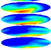
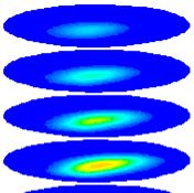
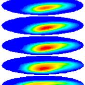
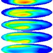
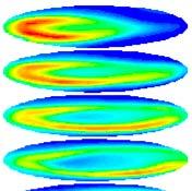
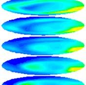
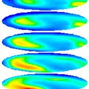
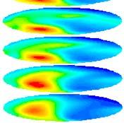
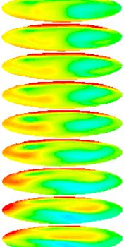
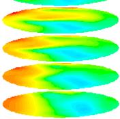
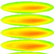
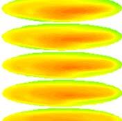
182 162 Table 6.2 Predicted axial eddy diffusivity in bubbly flow D C (cm) U g (cm/s) Computed D zz (cm 2 /sec) D zz (cm 2 /sec) Sparger 6A Sparger 6B Figure s 1 s 2 s 4 s 8 s 16 s 40 s Time evolution of the liquid tracer concentration inside a 44-cm diameter column at U g =10 cm/s.