Lecture 5: Classification

Transcription

1 Lecture 5: Classification Advanced Applied Multivariate Analysis STAT 2221, Spring 2015 Sungkyu Jung Department of Statistics, University of Pittsburgh Xingye Qiao Department of Mathematical Sciences Binghamton University, State University of New York 1 / 85

2 Outline 1 Example: Fisher s iris data 2 Bayes Rule, LDA & QDA 3 Logistic Regression 4 Assessment of classifiers 5 Software 6 More classifiers 2 / 85

3 Classification and Discriminant Analysis Data: {(x i, y i ) : i = 1,..., n} with multivariate observations x i R p (continuous) and population labels or class information y i = 1,..., K (categorical). Assume X (Y = k) F k, for different distributions F k. Binary classification: If there are only two cases, may write X 1,..., X n1 i.i.d. F 1 and Y 1,..., Y n2 i.i.d. F 2. Classification aims to classify a new observation, or several new observations into one of those classes (groups, populations). A classifier (classification rule) is a function φ(x) : X {1,..., K}. 3 / 85

4 The next section would be Example: Fisher s iris data 2 Bayes Rule, LDA & QDA 3 Logistic Regression 4 Assessment of classifiers 5 Software 6 More classifiers 4 / 85

5 Example: Fisher s iris data Fisher s iris dataset. Classification of flowers into different species (setosa, versicolor, virginica) based on lengths and widths of sepal and petal (4 variables). n = 150 observations Sepal.Length setosa versicolor virginica Sepal.Width Petal.Length Petal.Width / 85

6 Example: Fisher s iris data Focus on the latter two labels (red and green) Sepal.Length setosa versicolor virginica Sepal.Width Petal.Length Petal.Width / 85

7 Example: Fisher s iris data Try dimension reduction. Focus on the first two principal component scores PC1 setosa versicolor virginica PC PC3 PC / 85

8 Example: Fisher s iris data Species versicolor virginica PC PC2 8 / 85

9 Example: Fisher s iris data An example of classifier given by a linear hyperplane. φ(z) : R 2 {versicolor, virginica}, where { versicolor, b z < 0; φ(z) = virginica, b z 0, assuming no intercept b = ( 1.55, 3.06) Species versicolor virginica PC / 85

10 Example: Classifiers The previous example on classifying Fisher s iris data is an example of linear classifier. A linear classifier φ(x) is a function of linear combinations of input vector x and is of the form φ(x) = h(b 0 + b x). In binary classification (K = 2), the linear classifier may be written as φ(x) = sign(b 0 + b x) : b 0 + b x > 0 +1 Class; b 0 + b x < 0 1 Class R p is divided by a hyperplane { x : b 0 + b x = 0 } Moreover, a classifier may be quadratic, and beyond. φ(x) = h(b 0 + b x, x C x), 10 / 85

11 The next section would be Example: Fisher s iris data 2 Bayes Rule, LDA & QDA Bayes Rule Fisher s Linear Discriminant Exaples of LDA and QDA 3 Logistic Regression 4 Assessment of classifiers 5 Software 6 More classifiers 11 / 85

12 Setup Assume K = 2 for simplicity X (Y = 1) f 1 (x), X (Y = 2) f 2 (x). Denote a random observation from this population (a mixture of two populations) by (X, Y ). We assume P(Y = 1) = π 1, P(Y = 2) = π 2, π 1 + π 2 = 1 If the observed value of X is x, then Bayes theorem yields the posterior probability that the observed x was from the population 1: f 1 (x)π 1 η(x) := P(Y = 1 X = x) =. f 1 (x)π 1 + f 2 (x)π 2 12 / 85

13 0-1 Loss and Bayes (decision) rule Use a decision theory framework, if we care about the 0-1 loss: 1 {Y δ(x )}, we would hope to choose a decision function to minimize the risk associated with the 0-1 loss. E[1 {Y δ(x )} ] = Pr[Y δ(x )] We only need to choose a best decision δ(x) for each given X = x, that minimizes Pr[Y δ(x) X = x] Rewrite Pr[Y δ(x) X = x] =Pr[1 δ(x) X = x, Y = 1]P(Y = 1 X = x) + Pr[2 δ(x) X = x, Y = 1]P(Y = 2 X = x) The blue parts are either 0 or 1. Hence we only need to choose δ(x) to be the class j with greater P(Y = j X = x) 13 / 85

14 Bayes Rule Classifier for Gaussian The derivation from the last page is how we find the Bayes (decision rule): Bayes Rule classifier assigns the class label (1 or 2) which gives the higher posterior probability: φ Bayes (x) = argmax P(Y = k X = x). k=1,2 Now assume Gaussian data: X (Y = 1) N p (µ 1, Σ), X (Y = 2) N p (µ 2, Σ), µ 1 µ 2. Recall that η(x) := P(Y = 1 X = x) = f 1 (x)π 1 f 1 (x)π 1 + f 2 (x)π / 85

15 Bayes Rule Classifier: Gaussian 1-D As a special case, assume p = 1 and X (Y = 1) N 1 (µ 1, σ 2 1), X (Y = 2) N 1 (µ 2, σ 2 2), µ 1 µ 2. Then P(Y = i X = x) 1 exp( (x µ i ) 2 )π 2πσ 2 i i 2σ 2 i 0.4 equal variance, π 1 = 1/ unequal variance, π 1 = 1/ equal variance, π 1 = 2/ / 85

16 Bayes Rule Classifier: Gaussian 1-D The Bayes classifier classifier classify a point x into class 1 (blue) 1 case I (σ 1 = σ 2, π 1 = π 2 ): if 2 case II (σ 1 < σ 2, π 1 = π 2 ): if ( x µ 1 σ case III (σ 1 = σ 2, π 1 > π 2 ): if ( x µ 1 σ 2 1 x µ 1 < x µ 2. ) 2 < ( x µ 2 σ2 2 ) 2 + log(σ2/σ 2 1 ). ) 2 < ( x µ 2 σ2 2 ) log(π 1 /π 2 ). 16 / 85

17 More General Bayes Rule Classifier In general, for k = 1,..., K > 2. If the observed value of X is x, then Bayes theorem yields the posterior probability that the observed x was from the population k: P(Y = k X = x) = f k(x)π k f (x), where f k is the conditional density function of X (Y = k). Bayes Rule classifier assigns the class label (among 1,..., K) which gives highest posterior probability: Gaussian Example: φ Bayes (x) = argmax P(Y = k X = x). k=1,...,k X (Y = k) N p (µ k, Σ k ), k = 1,..., K, K P(Y = k) = π k, π k = 1, k=1 X f (x), a mixture density for multivariate normals 17 / 85

18 See that More General Bayes Rule Classifier for Gaussian Data φ Bayes (x) = k iff P(Y = k X = x) P(Y = i X = x) for all i, which is equivalent to 1 2 (x µ k) Σ 1 k (x µ k) log Σ k log(π k ) 1 2 (x µ i) Σ 1 i (x µ i ) log Σ i log(π i ) for all i. Moreover, φ Bayes (x) = argmin k=1,...,k δ k (x), where δ k (x) = b 0k + b k x + x C k x, where b 0k = 1 2 µ k Σ 1 k µ k log Σ k log(π k ), b k = Σ 1 k µ k, C k = 1 2 Σ 1 k. 18 / 85

19 Sample Bayes Rule Classifier for Gaussian Data In practice, we do not know the parameters (µ k, Σ k, π k ). Given n observations (x ij, i), (i = 1,..., K), (j = 1,..., n k ), n = K k=1 n k, sample versions of the classifiers are obtained by substituting µ k with ˆµ k = x k, Σ k with Σ k = S k. Also ˆπ k = n k /n. The moment estimate of the Bayes rule classifier for Gaussian data is then φ(x) = argmin k=1,...,k ˆδ k (x), where ˆδ k (x) = b 0k b k x + x C k x, where b 0k = 1 2 x k S 1 k x log S k log(n k /n), b k = S 1 k x k, C k = 1 2 S 1 k. 19 / 85

20 Mahalanobis distance In a special case where Σ k Σ, π k = 1/K, for all k: The Bayes rule classifier boils down to comparing the quantity d 2 M (x, µ k) = (x µ k ) Σ 1 (x µ k ), which is called (squared) Mahalanobis distance. Mahalanobis distance d M (x, µ) measures how much x is away from the center of distribution N p (µ, Σ). The set of points with the same Mahalanobis distance is an ellipsoid. Replacing Σ with its estimator S, and x with the sample mean x, the squared Mahalanobis distance is proportional to Hotelling s T 2 statistic. 20 / 85

21 Special cases of Bayes Rule Classifier for Gaussian Data Equal covariance Σ k Σ: φ Bayes (x) = argmin k=1,2 δ k (x), where δ k (x) = b 0k b k x, where b 0k = 1 2 µ k Σ 1 µ k log(π k ), b k = Σ 1 µ k For Equal covariance Σ k Σ and binary classification (K = 2): φ Bayes (x) = 1 when or (µ 2 µ 1 ) Σ 1 (x µ 1 + µ 2 ) < log(π 1 /π 2 ), 2 v x v µ < log(π 1 /π 2 ), v = Σ 1 (µ 2 µ 1 ). 21 / 85

22 Sample Bayes Rule Classifier for Gaussian Data (with equal Cov. mat.) In practice, we do not know the parameters (µ k, Σ, π k ). Given n observations (x ij, i), (i = 1,..., K), (j = 1,..., n k ), n = K k=1 n k, a sample version of the classifiers are obtained by substituting µ k with ˆµ k = x k, Σ with Σ = S P (pooled sample covariance matrix). Also ˆπ k = n k /n. The moment estimate of the Bayes rule classifier with the equal covariance assumption is then φ(x) = argmin k=1,...,k ˆδk (x), where ˆδ k (x) = b 0k b k x, where b 0k = 1 2 x k S 1 P x k log(n k /n), b k = S 1 P x k. 22 / 85

23 So far, we have developed TWO classifiers for Gaussian Data Linear Discriminant Analysis (Sample) Bayes rule classifier with equal covariance. For binary classification, φ(x) = 1 if b (x x 1 + x 2 ) < log( n 1 ), 2 n 2 b = S 1 P ( x 2 x 1 ). In general, φ(x) = argmax(b 0k b k x), b k = S 1 P x k. k Quadratic Discriminant Analysis (Sample) Bayes rule classifier with unequal covariance (see pp 19). φ(x) = argmax(b 0k b k x + x C k x). k 23 / 85

24 Fisher s LDA LDA (the sample estimate of Bayes rule classifier for Gaussian data with equal covariance) is often referred to as R.A. Fisher s Linear Discriminant Analysis. His original work did not involve any distributional assumption, and develops LDA through a geometric understanding of PCA. The LDA direction u 0 R p is a direction vector orthogonal to the separating hyperplane, and is found by maximizing the between-group variance while minimizing the within-group variance of the projected scores. (u x 1 u x 2 ) 2 u 0 = argmax u R p u S P u 24 / 85

25 Since we have Note that (u x1 u x2) 2 [ S 1 P u SP u = u ( x1 x2)( x1 x2) u, from Theorem 2.5 in HS, u SP u u 0 = e.v.1{s 1 P ( x 1 x 2 )( x 1 x 2 ) } ( x 1 x 2 )( x 1 x 2 ) ] S 1 P ( x 1 x 2 ) = λs 1 P ( x 1 x 2 ) where λ = ( x 1 x 2 ) S 1 P ( x 1 x 2 ) which happens to be the greatest eigenvalue of [ S 1 P ( x 1 x 2 )( x 1 x 2 ) ]. Hence the solution of u 0 is actually u 0 = S 1 P ( x 1 x 2 ) 25 / 85

26 Fisher s LDA Geometric understanding Two point clouds, each with S i = I 2. u 0 b = S 1 P ( x 2 x 1 ). 26 / 85

27 u 0 S 1 P ( x 2 x 1 ) = ( x 2 x 1 ). (direction of mean difference) 27 / 85

28 Slanted clouds. Assumed to have equal covariance. 28 / 85

29 Mean difference direction not efficient, as S P ci / 85

30 Individually transform subpopulations so that both are spherical about their means. y ij = S 1/2 P x ij. 30 / 85

31 In transformed space, best separating hyperplane is the perpendicular bisector of line between means. Transformed normal vector b Y : ȳ 2 ȳ 1 = S 1/2 P ( x 2 x 1 ). Transformed intercept b 0(Y ) : (ȳ 1 +ȳ 2 )/2 = S 1/2 P ( x 1 + x 2 )/2. Transformed input x is classified to 1 if b Y (y b 0(Y ) ) < 0 y = S 1/2 P 31 / 85

32 Original input x = S 1/2 y is classified to 1 if P b Y (y b 0(Y ) ) < 0 S 1/2 P ( x 2 x 1 ) (S 1/2 P x S 1/2 P ( x 1 + x 2 )/2) < 0 S 1 P ( x 2 x 1 ) (x ( x 1 + x 2 )/2) < 0 32 / 85

33 Leads to Fisher s LDA (u 0 S 1 P ( x 2 x 1 ) ) by actively using covariance structure. 33 / 85

34 In the next four sets of examples, LDA vs QDA Examples Blue and red points represent observations from two different populations. Blue line is the separating hyperplane given by computing the sample LDA, and is a line perpendicular to LDA direction b = S 1 P ( x 2 x 1 ), and is the set {x R 2 : b (x x 1 + x 2 ) = log( n 1 )}. 2 n 2 Red curve represent the boundary of classification regions given by the sample QDA, and is {x R 2 : b 01 b 1 x + x C 1 x = b 02 b 2 x + x C 2 x}. 34 / 85

35 LDA vs QDA Ex.1 35 / 85

36 LDA vs QDA Ex.1 36 / 85

37 LDA vs QDA Ex.2 37 / 85

38 LDA vs QDA Ex.2 38 / 85

39 LDA vs QDA Ex.3 39 / 85

40 LDA vs QDA Ex.3 40 / 85

41 LDA vs QDA Ex.4 41 / 85

42 LDA vs QDA Ex.4 42 / 85

43 The next section would be Example: Fisher s iris data 2 Bayes Rule, LDA & QDA 3 Logistic Regression 4 Assessment of classifiers 5 Software 6 More classifiers 43 / 85

44 Logistic Regression model Logistic Regression is another model based method (we need to impose a model to the underlying distribution.) Binary classification case. Assume that Y = 0 or 1, esp. the occurrence of an event. Model: logit(η(x)) := log ( ) η(x) = b + β x = f (x), 1 η(x) where η(x) = Pr(Y = 1 X = x) and η(x) = Pr(Y = 0 X = x) and β R p is the coefficient vector (similar to b in the previous section.) Can show that η(x) = exp(f (x)) 1+exp(f (x)) and 1 η(x) = 1 1+exp(f (x)). 44 / 85

45 Conditional likelihood Data: {(x i, y i ), i = 1,..., n} Given X i = x i, the Y i is a Bernoulli random variable (conditionally) with parameter η(x). [recall that η(x) depends on b and β.] Conditional likelihood of (b, β) is n η(x i ; b, β) y i [1 η(x i ; b, β)] 1 y i i=1 Conditional log-likelihood of (b, β) is l(b, β) := = n {y i log(η(x i ; b, β)) + (1 y i ) log[1 η(x i ; b, β)]} i=1 n {y i log i=1 ( ) [ exp(f (x i )) + (1 y i ) log 1 + exp(f (x i )) exp(f (x i )) ] } 45 / 85

46 l(b, β) := = = = n {y i log(η(x i ; b, β)) + (1 y i ) log[1 η(x i ; b, β)]} i=1 n {y i log i=1 ( ) [ exp(f (x i )) + (1 y i ) log 1 + exp(f (x i )) n {y i f (x i ) log[1 + exp(f (x i ))]} i=1 n {y i (b + β x i ) log[1 + exp(b + β x i )]} i=1 The maximizer of l(b, β), say (b, β ) can be plugged into f (x; b, β) f (x) = b + β x exp(f (x i )) ] } 1 f (x) > 0 η(x) > 1/2 Y is more likely to be 1 2 f (x) < 0 η(x) < 1/2 Y is more likely to be 0 46 / 85

47 For simplicity, view (b, β ) as new β Search solution β to score equation Optimization l(β) = 0 Recall univariate Newton-Raphson method: find root of f (x) = 0. Iteratively do: x n+1 x n f (x n )/f (x n ) Motivated by Taylor expansion. Here: where l(β) = g(β, b) := β (k+1) β (k) [ l(β (k) )] 1 l(β (k) ), 2 l(β) is the Hessian matrix β β T 47 / 85

48 Calculations lead to l(β) = n x i {y i η(x i ; β)} = X(y η) (1) i=1 where η := (η(x 1 ; β),..., η(x n ; β)) T (2) l(β) = X(y η) T β (3) = X η β T (4) = XWX T (5) Note that η(x i ;β) = β T η(x i ; β)[1 η(x i ; β)]x T i. Hence η = WX T, where W = β T Diag{η(x i ; β)[1 η(x i ; β)]} 48 / 85

49 Write the N-R method as β (k+1) β (k) [ l(β (k) )] 1 l(β (k) ) (6) = β (k) + [XWX T ] 1 X(y η) (7) = [XWX T ] 1 XW[X T β (k) + W 1 (y η)] (8) = [XWX T ] 1 XWz (9) This is exactly the solution to weighted least square with design matrix X, response variable z and weights η(x i ; β)[1 η(x i ; β)]. One must update the response variable and the weight matrix for each iteration. Convergence is NOT guaranteed. W and XWX T must be invertible. Data separation issue: if two classes are well separated, all η(x i ) are too close to 0 or 1 W is almost 0 (trouble!) 49 / 85

50 LDA vs Logistic Regression Logistic Regression is less sensitive to nongaussian data. Logistic Regression beats LDA when nongaussian or the covariance is not equal LDA is subject to outliers. Logistic less efficient than LDA. The latter exploits the full likelihood while logistic regression uses conditional likelihood. Logistic regression needs large sample size to work well. LDA can be quite flexible. Both have big problem when p n. 50 / 85

51 Alternative coding for logistic regression Recall for y i = 0, 1 y i log ( exp(f (x i )) 1 + exp(f (x i )) ) [ + (1 y i ) log exp(f (x i )) This is equivalent to the following function for coding y i = ±1 ( ) 1 log = log (exp( y i f (x i )) + 1) exp( y i f (x i )) + 1 Logistic regression can be viewed as minimizing over (β, b) ] n log (exp( y i f (x i )) + 1) = i=1 n L(y i (β T x i + b)) i=1 51 / 85

52 Gradient descent optimization The gradient descent algorithm takes the following update iteratively to minimize f (ω): where 0 < γ 1 is step size. ω (k+1) ω (k) γf (ω (k) ) Compared to the Newton-Raphson method ω (k+1) ω (k) (f (ω)) 1 f (ω (k) ), the gradient descent method directly update the minimizing point toward the direction of smaller (smallest) value of f, while Newton-Raphson method essentially indirectly optimizes by finding the root of f (ω) = 0 The direction γf (ω (k) ) is different from (f (ω)) 1 f (ω (k) ). N-R should converge sooner than gradient descent. The latter may call for many iterations. 52 / 85

53 The goal is to minimize over ω = (β, b) f (ω) := n log[1 + exp( y i ω T x i )] i=1 whose gradient is n f exp( y i ω T x i ) (ω) := 1 + exp( y i ω T x i ) y i x i i=1 n { } 1 = 1 + exp( y i ω T x i ) 1 i=1 y i x i At each iteration, we calculate the gradient, and then update according to ω (k+1) ω (k) γf (ω (k) ) 53 / 85

54 The next section would be Example: Fisher s iris data 2 Bayes Rule, LDA & QDA 3 Logistic Regression 4 Assessment of classifiers 5 Software 6 More classifiers 54 / 85

55 Assessment of classifiers A classifier φ classifies any input x into a class label {1,..., K}. How do we assess the performance of classifier φ? Misclassification occurs if x is classified to label j, but was actually from class k j. For a mixed population (X, Y ), the total probability of misclassification for classifier φ: P(φ(X ) Y ) = K P(φ(X ) k Y = k)p(y = k), k=1 where P(φ(X ) k Y = k) is the conditional probability of misclassification given Y = k. Here the probability P on the left side is with respect to the distribution of (X, Y ). A classifier φ is optimal if it has the smallest t.p.m. compared to any other classifiers, i.e., P(φ(X ) Y ) P(ϕ(X ) Y ), ϕ Φ. 55 / 85

56 Total probability of misclassification Bayes rule classifier is optimal (when the distributions are known). If a classifier ˆφ is estimated from a finite sample D := {(x i, y i )}, the total probability of misclassification (t.p.m) is usually adapted to the t.p.m. conditional on D P( ˆφ D (X ) Y D). Clearly, this probability above is a random variable depending on D [different data D lead to different realized ˆφ D ( ) which have different (conditional) t.p.m.] When treating D as given (and fixed), this probability becomes a constant. Total probability of misclassification is also called generalization error, test error, etc. 56 / 85

57 Misclassification rates In practice, since the distribution of (X, Y ) is unknown, one cannot compute P. Instead, we consider a big test data set T = {(x j, y j ), j = 1,..., M}, which induces an empirical distribution. This empirical distribution assigns 1/M probability mass to each point (x j, y j ) in T. The probability of φ(x ) Y based on this empirical distribution is ˆP( ˆφ D (X ) Y D) = 1 M M 1 {φ(x j ) y j} j=1 which is an unbiased and consistent estimate of the true generalization error P( ˆφ D (X ) Y D) This is sometimes called misclassification rate. 57 / 85

58 We usually do not have the luxury to have a big test data set. The same sample is used for estimation of the classification rule φ and also for evaluation of the performance of φ. In these cases, we could either 1 divide the sample into training and testing sets; or 2 use cross-validation. 58 / 85

59 Training and testing sets Binary classification (K = 2). Divide inputs x 1,..., x m and y 1,..., y n into two groups X tr = {x 1,..., x m1, y 1,..., y n1 } (training) and X test = {x m1 +1,..., x m, y n1 +1,..., y n } (testing). (Sorry for the abuse of notation. y is not the class label here.) Estimate the classifier φ using X tr. Estimate the misclassification rate using X test. Use Confusion matrix, defined in the next slide. 59 / 85

60 Training confusion matrix True class Class 1 Class 2 Class 1 r classified to 11 r 12 Class 2 r 21 r 22 where r ij is the number of observations in the training sample which are classified to class i and are actually from class j. rij = n 1 + m 1 := N tr, thus Training misclassification rate = (r 12 + r 21 )/N tr. Testing confusion matrix True class Class 1 Class 2 Class 1 s classified to 11 s 12 Class 2 s 21 s 22 where r ij is the number of observations in the testing sample which are classified to class i and are actually from class j. sij = n n 1 + m m 1 := N test, thus Testing misclassification rate = (s 12 + s 21 )/N test. 60 / 85

61 Training and testing sets IRIS data example Figure: Left: Two classes (versicolor and virginica), n = 50, m = 50 total observations, together with the separating hyperplane by LDA. Right: n 1 = 25, m 2 = 25 training observations. 61 / 85

62 Training and testing sets IRIS data example Figure: Right: n 1 = 25, m 2 = 25 training observations, together with the separating hyperplane by LDA, estimated using only training observations. 62 / 85

63 Training and testing sets IRIS data example Figure: Right: The remaining points corresponding to the testing set are overlaid. 63 / 85

64 Training and testing sets IRIS data example Training confusion matrix for this particular choice of training set. True class Versicolor Virginica Versicolor 24 1 classified to Virginica 1 24 Training misclassification rate = (r 12 + r 21 )/N tr = 2/50 = 4%. 64 / 85

65 Training and testing sets IRIS data example Testing confusion matrix for this particular choice of training set. True class Versicolor Virginica Versicolor 23 0 classified to Virginica 2 25 Testing misclassification rate = (s 12 + s 21 )/N test = 2/50 = 4%. The testing misclassification rate is an estimate of the total probability of misclassification P( ˆφ(X ) Y ). May not be a good one since the sample size is too small. In most cases the tr. and testing sets are chosen in advance. In this example, testing and training sets are chosen at random. Different choice of sets will lead to different rates. 65 / 85

66 K-fold Cross Validation To minimize the randomness in the choice of training and testing sets, we repeat the process. One example is the K-fold cross validation. Figure: For ith fold, testing misclassification rate p i is computed, average of those p i is the estimate of the total probability of misclassification P( ˆφ(X ) Y ). 66 / 85

67 Leave-One-Out Cross Validation The N-fold cross validation, where N is the sample size, is called Leave-One-Out Cross Validation. Figure: For ith iteration, testing misclassification rate p i is computed, average of those p i is the estimate of the total probability of misclassification P( ˆφ(X ) Y ). 67 / 85

68 Note that for each fold, say V 1, and its complement V 1, we are not estimating the performance of ˆφ D on V 1, but are estimating the performance of ˆφ V 1 on V 1. Hence the estimated generalization error is biased. Larger K means each fold is smaller, and since only one fold is left out, the training set V 1 is closer to the full set D. Hence larger K means less biased estimate. On the other hand, as K N, V i s become too similar to each other. An extreme case is K = N. This makes it difficult for V i s to mimic the typical observations of a (n 1) data set from the true distribution (especially when N is itself small). Moreover, this makes the resulting CV estimator too much depend on the data D. Larger K means the estimated generalization errors (before taking average) are highly correlated and taking average does not help to reduce the variance. Smaller K means that the errors are less dependent, and taking average does help to reduce the variance 68 / 85

69 How many folds are needed? Often K = 10 For smaller data, perhaps 5 or 3. K-fold CV (K N) is different from N-fold CV in that: For a given data set, the N-fold CV is deterministic, since each observation is classified by a deterministic classifier. For a given data set, the K-fold CV depends on how the data are split into folds. An observation may be judged by a different classifier (trained from a different set of training data) due to a different way of splitting. Find a balance between bias and variance. If time is not an issue, try repeat the K-fold many times with random splitting. 69 / 85

70 Cross Validated Misclassification Rates 10-fold cross validation is used to estimate the probability of misclassification, for each data: classification methods LDA QDA IRIS Ex. 1 (Equal Cov.) Examples Ex. 2 (Unequal Cov.) Ex. 3 (Unequal Cov.) Ex. 4 (Donut) / 85

71 Expected generalization error P(φ(X ) Y ) is the generalization error for a given classifier φ( ). This describes the performance of φ( ). Often φ( ) is trained from sample D, hence we have GE D := P( ˆφ D (X ) Y D). This quantity measures the performance of ˆφ D (X ), which is indirectly a measure of the performance of a classification procedure / method (through its behavior on D.) A related quantity is GE := E[GE D ] = E[P( ˆφ D (X ) Y D)] where the expectation is with respect to the distribution of D and the probability P is with respect to the distribution of (X, Y ). This measures the average performance of the procedure / method. Hence this quantity is not specific to any sample. 71 / 85

72 The next section would be Example: Fisher s iris data 2 Bayes Rule, LDA & QDA 3 Logistic Regression 4 Assessment of classifiers 5 Software 6 More classifiers 72 / 85

73 LDA and QDA in R library(mass) data(iris) train <- sample(1:150, 75) table(iris$species[train]) z <- lda(species ~., iris, prior = c(1,1,1)/3, subset = train) # predictions predict(z, iris[-train, ])$class # true labels iris$species[-train] z <- qda(species ~., iris, prior = c(1,1,1)/3, subset = train) # predictions predict(z, iris[-train, ])$class # true labels iris$species[-train] 73 / 85

74 Logistic Regression in R Use glm function. > z <- glm(species ~., iris, family = binomial ) Warning messages: 1: glm.fit: algorithm did not converge 2: glm.fit: fitted probabilities numerically 0 or 1 occurre > Data separation issue in this data set. 74 / 85

75 The next section would be Example: Fisher s iris data 2 Bayes Rule, LDA & QDA 3 Logistic Regression 4 Assessment of classifiers 5 Software 6 More classifiers 75 / 85

76 Various classifiers There are thousands of classification methods available. Examples of simpler methods 1 Nearest Centroid classifier, 2 Naive Bayes classifier, 3 k-nearest Neighbor classifier, Examples of advanced methods 1 Support Vector Machines (SVM: Ch 11, Izenman), 2 Distance Weighted Discrimination (DWD: Marron and his colleagues), 3 Classification And Regression Trees (CART: Ch 9, Izenman). A nonlinear classifier can be obtained by using the kernel trick. (Section 11.3, Izenman) Some advanced classifiers and nonlinear classifiers will be introduced later in this course. 76 / 85

77 Nearest Centroid/ Naive Bayes classifier For two group classification (x 11,..., x 1n and x 21,..., x 2n ), the nearest centroid classifier is φ(x) = 1 if b (x x 1 + x 2 ) < 0, b = ( x 2 x 1 ), 2 sometimes called mean difference classifier; the Naive Bayes classifier is φ(x) = 1 if b (x x 1 + x 2 ) < 0, b = D 1 2 P ( x 2 x 1 ), where D P is the diagonal matrix consisting of diagonal elements of S P. This is a Bayes rule classifier (applied to Gaussian data; hence is LDA) assuming the (common) covariance matrix Σ is diagonal (a reason that it is called naive). 77 / 85

78 Nearest Centroid (Mean Difference) IRIS data example Figure: Mean difference direction b x 1 x 2 and its separating hyperplane. 78 / 85

79 Naive Bayes classifier IRIS data example Figure: Better classification by Naive Bayes (Naive LDA) and by LDA. 79 / 85

80 Naive Bayes classifier IRIS data example Figure: Better classification by Naive Bayes (Naive LDA) and by LDA. 80 / 85

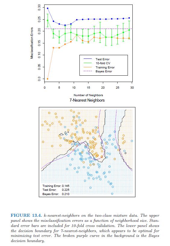
81 k-nearest-neighbor (k-nn) The k-nearest-neighbor classifiers are memory-based, and require no model to fit. Given a point x, we find k points x (r), r = 1,..., k, among training inputs, closest in distance to x. x is classified using majority vote among the k neighbors. simple to use. shown to be successful in examples. requires large memory if the dataset is huge. k chosen by comparing test error or cross validated error. not so useful for large p (as the concept of distance / neighbor becomes meaningless) 81 / 85

82 Example from ESL (Hastie, Ribshirani, Friedman) k-nearest Neighbor classifiers applied to a simulated data set, with three groups. The decision boundary of a 15-Nearest Neighbor classifier (top) is fairly smooth compared to a 1-Nearest Neighbor classifier (bottom). 82 / 85

83 Plug-in classifier Given a good estimator for η(x) := P(Y = 1 X = x), use a classifier defined as φ(x) := 1 [ η(x)>1/2] The idea of knn is essential to estimate P(Y = 1 X = x) by 1 k k j=1 y (j) where subscript (j) denotes the jth closest observation in the training data set to x. If the sample is dense enough, and if the sample size is large, then we expect that x (j) (j = 1,..., k) are all at x. Remember that Y X = x is simply a (conditional) Bernoulli random variable and its (conditional) expectation can be estimated by the sample mean (conditioning on X = x), 1 k k j=1 Y (j) k = 1, small bias, but large variance. Larger k, larger bias (because some of these neighbors may be far away from x), but smaller variance (because of the average). 83 / 85

84 84 / 85

85 k-nn in R library(class) data(iris3) train <- rbind(iris3[1:25,,1], iris3[1:25,,2], iris3[1:25,,3]) test <- rbind(iris3[26:50,,1], iris3[26:50,,2], iris3[26:50,,3]) cl <- factor(c(rep("s",25), rep("c",25), rep("v",25))) class<-knn(train, test, cl, k = 3, prob=true) mcr <- 1 - sum(class == cl) / length(cl) 85 / 85