THE RELATIVE IMPORTANCE OF HEAD, FLUX AND PRIOR INFORMATION IN HYDRAULIC TOMOGRAPHY ANALYSIS

Transcription

1 THE RELATIVE IMPORTANCE OF HEAD, FLUX AND PRIOR INFORMATION IN HYDRAULIC TOMOGRAPHY ANALYSIS Chak-Hau Michael Tso 1,5, Yuanyuan Zha 1,2, Tian-Chyi Jim Yeh 1, and Jet-Chau Wen 3,4* 1. Department of Hydrology and Water Resources, University of Arizona, Tucson, Arizona, U.S.A. 2. State Key Laboratory of Water Resources and Hydropower Engineering Science, Wuhan University, Wuhan, China. 3. Department of Safety, Health and Environmental Engineering, National Yunlin University of Science and Technology, Touliu, Yunlin, Taiwan, China. 4. Research Center for Soil and Water Resources and Natural Disaster Prevention, National Yunlin University of Science and Technology, Touliu, Yunlin, Taiwan, China. 5. Now at Lancaster Environment Centre, Lancaster University, Lancaster, U.K. * Corresponding author (wenjc@yuntech.edu) Highlights Flux data and head data carry non-redundant information about heterogeneity Flux measurements in addition to head data improve K estimates Estimates are less prone to uncertainty of prior K information when flux measurements are included This article has been accepted for publication and undergone full peer review but has not been through the copyediting, typesetting, pagination and proofreading process which may lead to differences between this version and the Version of Record. Please cite this article as an Accepted Article, doi: /2015WR017191

2 2 Research Significance This research leads to several significant findings: 1) information about hydraulic conductivity (K) embedded in head and flux measurements at the same location during hydraulic tomography (HT) are non-redundant; 2) joint interpretations of these measurements yield superior estimates of K heterogeneity, even when prior layering information is included; 3) as flux measurements are included in additional to head data in HT analysis, the estimates are less prone to uncertainty of prior information required in the analysis. Index Terms: 1829 Groundwater hydrology 1869 Stochastic hydrology 1894 Instruments and techniques: modeling 3260 Inverse theory Keywords: hydraulic tomography, groundwater, geostatistics, prior information, inverse modeling, flux

3 3 1 ABSTRACT Using cross-correlation analysis, we demonstrate that flux measurements at observation locations during hydraulic tomography (HT) surveys carry non-redundant information about heterogeneity that are complementary to head measurements at the same locations. We then hypothesize that a joint interpretation of head and flux data, even when the same observation network as head has been used, can enhance the resolution of HT estimates. Subsequently, we use numerical experiments to test this hypothesis and investigate the impact of flux conditioning and prior information (such as correlation lengths, and initial mean models (i.e. uniform mean or distributed means)) on the HT estimates of a non-stationary, layered medium. We find that the addition of flux conditioning to HT analysis improves the estimates in all of the prior models tested. While prior information on geologic structures could be useful, its influence on the estimates reduces as more nonredundant data (i.e., flux) are used in the HT analysis. Lastly, recommendations for conducting HT surveys and analysis are presented.

4 4 2 INTRODUCTION Detailed characterization of the spatial distribution of hydraulic properties of aquifers is crucial for high resolution prediction of water and solute movement in the subsurface [Yeh, 1992; Yeh et al., 1995a, 1995b; Mccarthy et al., 1996; Mas-Pla et al., 1997]. Traditional pumping tests and analysis yield either ambiguously averaged and scenario-dependent effective hydraulic parameters for equivalent homogeneous aquifers [Wu et al., 2005; Straface et al., 2007; Wen et al., 2010], or scenario-dependent distributed effective parameter fields that could vary with pumping locations (see Huang et al. [2011] and Wen et al. [2010]). As a consequence, results from traditional analysis can only be used as a first-cut approach for aquifer characterization [Yeh, 1992]. To minimize the impact of these problems, hydraulic tomography (HT) has been developed over the past two decades. While the HT concept had been proposed earlier [e.g., Gottlieb and Dietrich, 1995; Vasco et al., 1997; Butler et al., 1999], after the 3-D work by Yeh and Liu [2000] and Zhu and Yeh [2005], HT has emerged as a subject of active theoretical, laboratory, and field research to characterize the spatial distributions of hydraulic parameters at a higher level of detail (e.g. Yeh and Liu [2000]; Bohling et al. [2002; 2010]; Liu et al. [2002]; Brauchler et al. [2003, 2011, 2013]; Li et al. [2005, 2008]; Li and Cirpka [2006]; Zhu and Yeh [2005, 2006]; Illman et al. [2007, 2008, 2009, 2015]; Liu et al. [2007; 2011]; Straface et al. [2007]; Kuhlman et al. [2008]; Ni and Yeh [2008]; Cardiff et al. [2009, 2013b]; Castagna and Bellin [2009]; Xiang et al. [2009]; Berg and Illman [2011, 2013, 2014]; Cardiff and Barrash [2011]; Huang et al. [2011]; Liu and Kitanidis [2011]; Sharmeen et al. [2012]; Jiménez et al. [2013], Hochstetler et al. [2015] and Zhao et al. [2015]). In particular, Cardiff and Barrash [2011] provide a summary of all peer-reviewed HT studies (1D/2D/3D). These past research efforts have demonstrated that HT is a cost-effective, highresolution aquifer characterization method. Specifically, these studies have consistently

5 5 demonstrated that transient HT can identify not only the pattern of the heterogeneous hydraulic conductivity (K), but also the variation of specific storage (S s ) (see Zhu and Yeh [2005, 2006]; Liu et al. [2007]; Xiang et al., [2009] in particular). More importantly, it is also shown that the hydraulic property fields estimated by HT can lead to better predictions of flow and solute transport processes than conventional characterization approaches [Ni et al., 2009; Illman et al., 2010, 2012]. While HT is a relatively mature technology for characterizing aquifers, there remains room for improvement. HT s cost-effectiveness stems from collecting non-redundant information from a limited number of wells [Yeh and Lee, 2007; Yeh et al., 2008, 2014; Huang et al., 2011; Sun et al., 2013]. New approaches that collect additional non-redundant information at the wells used by HT experiments (i.e. without using new observation locations) would be the most appealing. For example, Lavenue and de Marsily [2001] analyze sinusoidal pumping tests conducted in a tomographic survey fashion in a fractured dolomite of the Rustler Formation within the Delaware Basin in southeastern New Mexico to characterize the K field in the Culebra Dolomite Formation. Cardiff et al. [2013a] promote the advantages of oscillatory hydraulic tomography for characterizing groundwater remediation sites. The fusion of different types of surveys (geophysical or tracer data), which may carry some non-redundant information about heterogeneity, offers another possible suite of approaches to address this issue. Nonetheless, recent studies have demonstrated that they can only provide some limited improvements, which can be attributed to additional uncertainty in the relationships between K and other physical attributes of other surveys (such as spatial variability of Archie s law, which links electrical resistivity to moisture content [see Yeh et al., 2002], and solute transport properties of tracers).

6 6 An alternative approach to improve the resolution of HT is to jointly invert steadystate depth-averaged drawdown HT data and the vertical profile of relative hydraulic conductivities based on prior flowmeter tests along fully screened observation wells (i.e., Li et al. [2008]). In other words, this particular approach overcomes the limitation of the depthaveraged head measurements at fully-screened observation wells by incorporating prior knowledge of vertical relative hydraulic conductivity variations from borehole flowmeter profiles. Li et al. [2008] report that such a joint inversion allow them to derive 3-D heterogeneity even though the observation wells are fully-screened. More recently, Yeh et al. [2011, 2015a, 2015b] and Mao et al. [2013b] discuss the necessary conditions for the inverse problems to be well-defined and advocate the importance of having K or flux measurements around the the perimeter of the pumping experiment field site. They are essential to constrain the inverse problems for the estimation of K and S s values, such that the problems are well defined. In addition, many existing monitoring wells in the field are fully screened and packed with gravel over a long interval. Head measurements at these wells represent some averaged head values over the interval, and they do not carry significant information about vertical aquifer heterogeneity [e.g. Li et al., 2008]. To overcome this problem, flux measurements along the well screen during HT surveys may offer a possible solution. This approach collects flux data along observation wells induced by the pumping of the HT survey, rather than the independently pumping at observation wells as in Li et al [2008]. Following this school of thought, Zha et al. [2014] develop a new approach that incorporates the flux measurements in HT analysis; and this new approach is then applied to 2-D synthetic fractured rocks. They show that inclusion of flux measurements could lead to significant improvements in the estimates of fracture conductivity and fracture distribution if a large number of measurements are available. Their study confirms the necessary conditions

7 7 that are discussed by Yeh et al. [2011, 2015a, 2015b] and Mao et al. [2013b]. Nevertheless, such benefits of flux measurements in more continuous 3-D porous media and impacts of prior information used in HT analysis need to be explored. The objective of this paper, therefore, is to investigate the improvements of hydraulic conductivity (K) estimates based on a joint interpretation of head and flux measurements during HT tests in a 3-D non-stationary heterogeneous aquifer, as well as to study the influence of prior information on these improvements. We first start with a brief description of the Simultaneous Successive Linear Estimator (SimSLE) method for HT analysis using both head and flux measurements in section 3.1. Then, we discuss in section 3.2 the associated cross-correlation analysis, which is used to explain the information about heterogeneity carried by head or flux measurements. This is followed by a description of the setup for numerical experiments (section 4.1). In section 4.2, we show results from threedimensional cross-correlation analysis between K and head and that between K and flux. We then conduct HT inversions in section 4.3 with and without flux conditioning on the synthetic K field and examine the effects of prior mean, correlation lengths, and uncertainty in prior models on the benefits of flux conditioning. Results from these experiments and their relevance to field applications are then discussed (section 5). In section 6, we summarize our findings and provide recommendations for conducting HT survey and analysis. 3 METHODS 3.1 Simultaneous Successive Linear Estimator (SimSLE) For the HT analysis in this study, we adopt the steady-state HT technique with flux conditioning developed by Zha et al. [2014], which is based on the SimSLE (Simultaneous SLE) algorithm [Xiang et al., 2009]. The SimSLE approach is basically the same as the SLE (successive linear estimator) developed by Yeh and colleagues [Yeh et al., 1996, 2002, 2006;

8 8 Zhang and Yeh, 1997; Hughson and Yeh, 2000; Yeh and Liu, 2000; Zhu and Yeh, 2005; Yeh and Zhu, 2007], with the extension that it simultaneously considers the observations from multiple pumping/injection events. SLE conceptualizes the natural logarithm of hydraulic conductivity (lnk=f) as a spatial stochastic process, characterized by prior information (i.e., mean, variance, and spatial correlation function). It assumes that the correlation function is an exponential correlation function with correlation scales λx and λ y in the horizontal directions, and λ z, in the vertical direction. Similarly, head (H), and the magnitude of flux (q), are also treated as spatial stochastic processes. These stochastic processes can be expressed as the sum of the unconditional mean and the unconditional perturbation (i.e., H( x) = H( x) + h( x ), q( x) = q( x) + v( x ), and F ( x) = F( x) + f ( x ) ). The unconditional mean head, H ( x ), and flux, q( x ), are derived from solving the ensemble mean steady groundwater flow equation with a given F( x ). The ensemble mean equation is a combination of Darcy s law and mass conservation in a continuum: subject to the boundary conditions qx ( ) + Q( x ) = 0, qx () = K() x H() x (1) p H = H, Γ 1 0 q n = q Γ1 0 (2) In the above equations, x = (x,y,z), [L], where x, and y are in the horizontal plane and z is positive upward; K(x) is the saturated hydraulic conductivity [L/T], H is the total head [L], q is the Darcian flux or the specific discharge (q = [q x, q y, q z ], [L/T]), and Q(x p ) is the flow rate at a source/sink at the location x p. q or q is the magnitude of flux. Γ1 and Γ 2 are prescribed head and flux at the Dirichlet and Neumann boundary, respectively. For the finite

9 9 element analysis, the solution domain for Eqs. (1) and (2) is discretized into N elements, such that the parameter K field is written as a vector f (N 1) and in turn, <F(x)>. Equations (1) and (2) are solved using the finite element code VSAFT3 (Variably SAturated Flow and Transport in 3-D) developed by Srivastava and Yeh [1992]. Suppose we have collected m h observed head, H and m q observed flux perturbations, q, during an HT survey which consists of several pumping tests. Thus, the observed data vector d (m 1, where m= m h + m q ) is composed of m h head data values and m q flux data sets. We then employ a stochastic linear estimator (Eq. 3) to improve the unconditional mean ln K(x) by using observed data set. Since the relationship between parameter K and head is nonlinear, a successive iteration scheme [Yeh et al., 1996] is adopted here to fully exploit the information about K conveyed in the head data sets. That is, ( ) Fˆ Fˆ ω d d (3) ( r +1 ) ( r) ( r) T ( r) c = c + In Eq. (3), ˆ ( r ) c F is an N 1 vector representing the estimate of <F(x)> c, given the observed data set (conditioning denoted by the subscript c), r is the iteration index. When r = 0, the estimate starts from an initial guess (prior information) of the K field (unconditional mean K, in general). Afterwards, the estimate of the conditional mean <F(x)> c is successively improved by the weighted difference between d (the observed data) and the vector ( r) d (the simulated data). This simulated data is obtained from the conditional mean equation (Eq. (1)) using the estimate of the conditional mean ˆ ( r ) c F at the iteration r. The coefficient matrix ω (m N) in Eq. (3) is determined by solving the following equation: [ + +θdiag( )] ε Q ε ω =ε (4) dd d dd df

10 10 where ε dd is the conditional covariance matrix (m m) between the secondary data (i.e., head, flux magnitude, or flux vector) sets, and ε df is the conditional cross-covariance matrix (m N) between the secondary data sets and the parameter f representing the conditional perturbation of the lnk(x) field. In Eq. (4), θ is a stability multiplier and diag( ε dd ) is a stability matrix, which is the diagonal elements of the ε dd measurement errors, unresolved heterogeneity, and others. matrix, and Q d is a diagonal matrix of variances of In Eq. 4, estimates of covariance matrix εdd and cross-covariance εdf matrix are required. They can be approximated by using 1 st -order Taylor s expansion to obtain ε = J ε J and ( r) ( r) ( r) ( r) T dd df ff df ε = J ε respectively, where ( r) ( r) ( r) df df ff ( r) Jdf is the sensitivity (or Jacobian) matrix for the observed data with respect to f using the set of estimated parameters at the r-th iteration. At r = 0, the covariance matrix for parameters ε ff is unconditional and is essentially the spatial covariance matrix R ff. It can be obtained using a user-specified covariance function. In the subsequent iterations, the covariance matrices become conditional (or residual) covariance given the observations and are updated to reflect the successive improvements in the estimates: ε = ε ω ε (5) ( r+ 1) ( r) ( r) T ( r) ff ff df Mathematically, this updating procedure is similar to that in the Kalman filter algorithm [e.g. Schöniger et al., 2012] as new information is included. However, this update is applied to reflect the change in cross-correlation between head and parameters due to improved conditional mean parameters during each iteration. The adjoint sensitivity formulation for SimSLE used in this work can be found in Zha et al. [2014].

11 Cross-correlation Analysis Formulation Cross-correlation analysis is a weighted sensitivity analysis casted into a stochastic framework [Mao et al., 2013a]. It determines the relative impact of each parameter with respect to others in time and space on the observed heads according to uncertainty or spatial variability of each parameter. The cross-correlation matrix can be obtained by: 1/2 ( ) diag( ) 1/2 ρdf = diag ε dd εdf ε ff (6) Each row of the cross-correlation matrix ρdf defines the fractional contribution from the uncertainty of data at the given observation location, which are carried forward to parameter estimation uncertainty of each element in a geostatistical sense. Since this crosscorrelation analysis is conducted without conditioning on any data, ε ff is replaced by its unconditional counterpart R ff. Consequently, ε df and εdd are determined by R ff and the unconditional mean K. With a given mean K, a pumping rate, and boundary conditions, these cross-covariances are evaluated numerically using the first-order analysis discussed earlier. The above cross-correlation analysis in heterogeneous aquifers is similar to the sensitivity analysis by Oliver [1993] but it adopts the stochastic or geostatistics concept. In particular, the cross-correlation analysis considers the variance (spatial variability) of the parameter and its spatial correlation structure (covariance function of the parameter) in addition to the most likely flow field considered in the sensitivity analysis. Physically, the correlation structure represents the average dimensions of aquifer heterogeneity. The crosscorrelation in essence represents the statistical relationship of spatial variability (or uncertainty) of a given parameter (K) at any location and the variability (or uncertainty) of head or flux at an observation location in the aquifer. Therefore, if the cross-correlation pattern between an observed head at a location and K everywhere is different from that between an observed flux at the same location and K, then the head and flux carry non-

12 12 redundant information about K distribution in the aquifer. Inclusion of these different data sets will be useful for HT analysis. The above cross-correlation analysis is also similar to the interpolation splines used by Kitanidis [1998], Snodgrass and Kitanidis [1998], and Fienen et al. [2008]. Note that the cross-correlation is the foundation of the cokriging approach [e.g. Kitanidis and Vomvoris, 1983; Hoeksema and Kitanidis, 1984; Yeh et al., 1995b; Yeh and Zhang, 1996; Li and Yeh, 1999], the nonlinear geostatistical inverse approach [e.g. Kitanidis, 1995; Yeh et al., 1996; Zhang and Yeh, 1997; Hanna and Yeh, 1998; Li and Yeh, 1998, 1999; Hughson and Yeh, 2000], the HT inverse model [e.g. Yeh and Liu, 2000; Zhu and Yeh, 2005], and the geostatistical inverse modeling of electrical resistivity tomography [Yeh et al., 2002]. 4 NUMERICAL EXPERIMENTS 4.1 Experimental Setup The synthetic aquifer that is used for the following numerical experiments is 45 m in length, 45 m in width and 18 m in depth (Figure 1a). The well configuration and design are identical to those at the North Campus Research Site (NCRS) in Waterloo, Ontario, Canada [Berg and Illman, 2011]. Results from the analysis herein may help in the assessment of previous field experiments and the design of future experiments at the site. The 15 m 15 m 18 m well array is set up in a nine-spot square pattern such that the centers of the well array and the synthetic aquifer coincide. It consists of four continuous multichannel tubing (CMT) wells containing seven channels as observation ports, and five multilevel pumping wells (PW) containing three to five channels (Figure 1b). For the CMT wells, the screens are spaced 2 m apart with the upper most screens located between 4.5 and 5.5 m below-ground surface (mbgs), and the deepest screens are set at 16.5 to 17.5 mbgs.

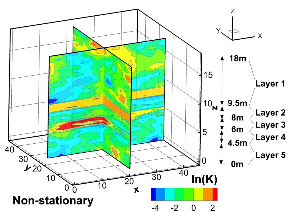
13 13 This aquifer is discretized into 26,353 nodes that form 23,328 rectangular elements. The dimensions of each element are 2.5 m (length) x 2.5 m (width) x 0.25 m (high). The side boundaries of the aquifer are identical constant head boundaries of 100 m, while the top and bottom boundaries are no-flow. We then generate K values for each element such that the K values in the entire aquifer represent a non-stationary random field with five alternating layers of aquifers and aquitards, which is analogous to the geologic characteristics of the NCRS. The K field consists of 5 horizontal layers (Figure 2) layer 1 is from z = 18 m to 9.5 m, 8.5 m thick; layer 2 is from z = 9.5 m to 8 m, 1.5 m thick; layer 3 is from z = 8 m to 6m, 2m thick; layer 4 is from 6 m to 4.5 m; 1.5 m thick; and layer 5 is from z = 4.5 m to 0 m. For each of the layers, independent random fields of K are generated individually using the random field generator. The mean lnk (m/d) or each of the layers, from layer 1 to layer 5, is , , , , and , respectively, and the variance of lnk for each corresponding layer is 2.5, 0.1, 1.0, 4.0, and 2.0, respectively. The horizontal correlation lengths for each layer are 10 m, while the vertical correlation length is 3 m for layer 1 and layer 5, and 0.5 m for others. The overall mean is , while the overall variance is Notice that layer 2 is a highly permeable layer with very small variability, and layer 4 is also a layer of high permeability but high variability. After generating the random K field with these spatial statistics, steady-state responses of the aquifer under a HT survey are simulated. The HT survey uses the same set of pumping rates and locations as Berg and Illman [2011]. During each pumping test, head (H) and flux data are collected at observation ports (see Figure 1b). The pumping and observation locations are the same as Berg and Illman [2011], which are listed in supplementary information Table S1, while the pumping rates are in Table S2. The HT experiment is designed in such a way in order to guide the field experiments at NCRS.

14 Cross-correlation Analysis For flux measurements to improve HT estimates, they must possess additional and non-redundant information on K heterogeneity to that provided in head measurements collected at the same location. This non-redundancy of the flux data can be demonstrated by comparing the cross-correlations between the flux magnitude at a location and K everywhere in the aquifer ( ρ qf ), and that between H and K ( ρ Hf ). In order to investigate these cross-correlations, we used a pumping-observation well couplet in the synthetic aquifers with the same boundary conditions as discussed in previous sections. The couplet includes a pumping port (PW), located at x = 22.5 m, y = 15 m and z = 9 m, and a head and flux measurement port (OW) at x = 22.5 m, y = 30 m and z = 9 m. The pumping rate is given as 2.5 m 3 /d, and the flow field is at steady state. The mean K field used is m/d and variance of lnk is 0.1. We first assume the correlation lengths in x, y, and z-directions to be 1m. The 3-D isosurfaces of the cross-correlations between K and head, flux magnitude, and flux vectors are shown in Figure S1. While the 3-D cross-correlation pattern between K and head and flux is new, the pattern and physical explanations are very similar to those presented in other recent work. (i.e. 1-D head examples [Yeh et al., 2014], 2-D head examples [Mao et al., 2013a; Sun et al., 2013]; 2-D flux example [Zha et al., 2014], and 3-D head examples [Mao et al., 2013a]). Next, we explore the cross-correlation patterns between head and K, and between flux and K under different mean K distributions. In Figure 3, the horizontal and vertical correlation lengths in x, y, and z-directions in all cases are assumed to be 10 m, 10 m, and 2.5

15 15 m respectively. For the ease of comparison, we report only the cross-correlation contours of the vertical cross-section that bisects PW and OW. Figures 3a and 3b show the cross-correlations for a uniform assumed mean K. In Figure 3a, the cross-correlation between head and K is the highest upstream of PW near the left boundary and upstream of OW near the right boundary. As shown in Figure 3b, the crosscorrelation between flux and K is the highest at OW and decreases concentrically away from it according to the correlation scales in the horizontal plane. We repeat the cross-correlation analysis by moving OW down to z = 4 m (Figure 3c-d). As expected, since a uniform mean is assumed, the change in cross-correlation patterns only corresponds to the change in OW location. We now proceed to examine the cross-correlation between head and lnk (Figure 3e), as well as flux and lnk (Figure 3f) respectively when a layered K field is assumed. Each layer is homogeneous, and layer locations and the mean K values are identical to those for the 5 zones of the reference field (Figure 2). The horizontal and vertical correlation lengths in x, y, and z are assumed to be 10 m, 10m, and 2.5 m respectively, and the variance of lnk for all layers is 0.1. When comparing Figure 3e with 3a, and Figure 3f with 3b, we notice the magnitude of cross-correlation becomes higher at elevations near to that of PW and OW, while it becomes smaller near the top and bottom of the domain. We attribute such behavior to the fact that the two wells are located in the same highly permeable layer, which suggests flow is predominately parallel to the layer boundaries. We also repeat the cross-correlation analysis by moving the OW down to 4 m. The head and K cross-correlation (Figure 3g) changes slightly but high cross-correlation areas remain in the high permeability zone, even though the OW is at the low permeability zone. The flux and K cross-correlation (Figure 3h), however, drops to close to zero everywhere. Such behaviors suggest that the flux measurements carry information highly pertinent to the

16 16 connectivity between pumping location and observation location. This finding corroborates the work by Zha et al. [2014], which demonstrates that flux measurements can enhance mapping of fractures significantly. The above finding also has important implications to the HT estimates of the layered system in next section. 4.3 HT ANALYSIS In this section, we discuss the use of simulated head data or both head and flux data from the numerical experiments and SimSLE to estimate the reference K field (Figure 2), with different types of prior information. The aim of this analysis is to evaluate the relative importance of observed data (head or head and flux) and prior information required by SimSLE and other geostatistically based models Prior Information Cases The prior information for SimSLE consists of a mean and a covariance function. The covariance function is a statistical representation of the average shape of the heterogeneous field to be estimated. The covariance function comprises variance, autocorrelation function, and spatial correlation scales, λ x, λ y, and, λ z in x, y, and z directions, respectively, of the parameter field. These correlation scales are analogous to the average dimensions (i.e., length, thickness, and width) of the heterogeneity in the entire domain. For mathematical convenience, the autocorrelation function is commonly assumed to be an exponential function. For this non-stationary reference K field, we will consider two approaches to the prior information: in Case 1, we treat the K field to be estimated as a stationary random field, with a uniform mean; and in Case 2, we treat it as a nonstationary random field with distributed means.

17 Case 1a and Case 1b Two scenarios are considered in Case 1. A geostatistical inversion generally starts with a uniform mean model the field is taken to be homogeneous before it is conditioned on measurements to estimate perturbation of parameters about the mean. This represents the case in which we have no knowledge about the presence of site-specific geologic structure(s) or trend of K in a field site. With a given mean value of the entire K field, we derive the estimates from HT data in Case 1a, assuming short horizontal correlation scales (i.e., λ x = λ y = 10 m, λ z = 2.5 m), i.e., we underestimate the true correlation scales of the entire domain. In Case 1b, we assume long horizontal correlation scales (i.e., λ x = λ y = 50 m, λ z = 2.5 m) to represent our prior knowledge about the stratified reference K field Case 2 Case 2 also considers several possible scenarios (Cases 2a, 2b, 2c, and 2d). In practice, geologic cross-sections based on well logs or geophysical surveys can reveal some layering structures in an aquifer. This information can serve as our prior knowledge about the site-specific distribution of mean K values (e.g., a layer of coarse sand overlying a layer of silty clay sand or vice versa) at a site. As a consequence, in Case 2a, we assume that the prior distributed model has perfect information about the layering. That is, it consists of the 5 zones identical to that used in the reference field generation. Each of the zones is homogeneous with a known mean K value identical to that of the corresponding layer in the reference K field. In Case 2b, we examine the effects of imprecise prior information on layer boundaries, while the mean for each layer is known exactly. That is, we repeat the runs for the distributed mean K field using a smoothed layered initial guesses, rather than precise ones as in Case 2a. The smoothing is done by shifting the position of the four layer boundaries about the

18 18 reference ones by an arbitrarily chosen perturbation function: Δ = cos(0.4 x )cos(0.2 y ), where e e e Δ e, rounded to the nearest integer, is the number of elements shifted vertically, while x e and ye are element numbers in the horizontal directions. Commonly, true mean K value of each layer is not known based on geologic or geophysical investigations. Point measurements of K from core samples or slug tests are usually used to estimate the mean of each layer. These mean estimates are likely to be different from the true means. Therefore, in Case 2c, we will consider that the layer boundary is known exactly but the mean K values are assigned from point measurements and different from the true means. On the other hand, Case 2d represents the scenario where both the boundary and the means are uncertain. The assigned mean lnk (m/d) value for each of the layers in Case 2c-d is, from layer 1 to layer 5, , , , , , respectively, as compared with those in the reference field ( , , , , and ). For all scenarios in Case 2 (i.e., 2a-d), we also examine effects of both small horizontal correlation scales (i.e., λ x = λ y = 10 m, λ z = 2.5 m) and large horizontal correlation scales (i.e., λ x = λ y = 50 m, λ z = 2.5 m). Generally, since large-scale geologic structures have already been depicted by the distributed means, using a smaller horizontal correlation scales should facilitate characterization of small-scale heterogeneity within layers [Ye et al., 2005] Performance Metrics To evaluate the HT estimates with either head or both head and flux data with different pieces of prior information, scatter plots of the estimated vs. true K values for each case are plotted, and a linear model is then fitted to each case without forcing the intercept to zero. The slope and intercept of the fitted linear model, the coefficient of determination (R 2 ),

19 19 the mean absolute error (L 1 ), and the mean square error (L 2 ) norms are then used as performance metrics for evaluation since a single criterion is not sufficient. The L 1 and L 2 norms are computed as: n 1 L1 = ln Ki ln Ki and N i= 1 1 L2 = K K N n 2 (ln i ln i) (7) i= 1 where N is the total element of the model, i indicates the element number, K i is the estimated K value for the i-th element, and K is the true K value of the i-th element. i In general, the smaller values for L 1 and L 2 are, the better the estimates are; the closer the slope of the linear regression line to 1 and the intercept to 0, the better the estimates are. Similarly, if R 2 value is close to 1, the estimate is considered to be better Results Performance metrics for results of all cases and scenarios using head and head/flux data are listed in Table 1. For clarity, we will discuss only selected cases and scenarios below Head Inversion Figure 4 displays the contour cross-sections and scatter plots along with the performance metrics of the estimated K field from head inversion. Figures 4a-b are estimates from using uniform mean and short correlation lengths as prior (Case 1a), Figures 4c-d are those using uniform mean and long correlation lengths (Case 1b), while Figures 4e-f show the results using a perfect distributed mean (Case 2a) and short correlation lengths. When only head data are used, the estimates based on short correlation scales and uniform mean as prior information (Figures 4b) are largely biased (i.e., slopes deviating from 1 and large

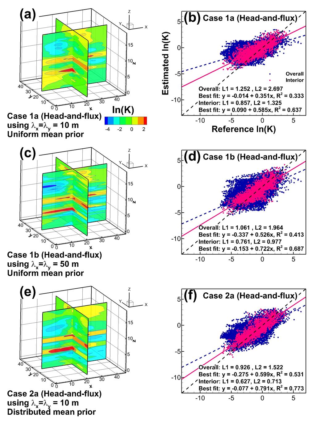
20 20 intercepts) for both the entire field and the interior field. The estimated K field (Figure 4a) successfully resolves the top aquifer (i.e. layer 2), yet most of the other features in the reference field are unresolved. On the other hand, when the long correlation scales and uniform mean are used as the prior information, the bias and errors of the estimates both drop drastically (Figure 4d). This reduction in bias is clearly reflected in all performance metrics. In particular, the L 2 drops from to for interior points and from to overall. The use of the long correlation scales as prior information in essence permits SimSLE to closely reproduce the head field in the layered medium, such that the final estimated field is more layer-like (Figure 4c). However, the estimates still cannot capture the true variability of the reference field, as manifested by the large envelope of spread of both the overall and interior scatter points. In particular, the shape of the high permeability layer 4 is not clearly identified. When a distributed mean is used alongside with the assumed short correlation lengths as prior, the K estimates from head inversion improve greatly (Figure 4f), while the bias and error of the estimates reduce remarkably. The layering, as expected, is better recovered given the correct distributed prior (Figure 4e). That in turn has helped local features within the well field to be better reproduced. Head inversion results from using noisy distributed mean prior models (Case 2b-d) with short horizontal correlation scales are illustrated in Figure S2 of the supporting information section Head-and-flux Inversion We next examine the effects of prior information on the estimates when both head and flux data are used (Figure 5). Figures 5a and 5b are the contour map and the associated scatter plot, respectively, of estimates from using uniform mean and short correlation lengths

21 21 as prior (as in Case 1a). The same plots for estimates from using the same uniform mean and long correlation lengths (as in Case 1b) are shown in Figures 5c and 5d. Similarly, Figure 5e and 5f illustrate those based on the precise distributed mean and short correlation lengths (as in Case 2a). When the uniform mean with the long correlation lengths are used, the estimates in the whole domain as well as the interior of the well field are less biased in Figure 5d than those in Figure 5b. This reduction in bias is well manifested when the slopes and intercepts of the blue dashed lines and red solid lines in the scatterplots are compared. The L 2 also drops from to for interior points and from to for overall. Notice that the scattering of the red points in both Figures 5b and 5d appears to be satisfactory. However, the large scatter envelop of the blue points in Figure 5d, seems to indicate that much of the smallscale variability outside the well field remains undetermined when long correlation scales are used. According to the contour plots of the estimates in Figures 5a and 5c, the head-andflux inversion with a uniform mean and short or long horizontal correlation scales as prior generally resolves the layering features of the non-stationary reference K field. However, assuming short correlation lengths leads to estimates with too many lenses (Figure 5a) and assuming long ones overestimates the lateral extents of the high permeability zones (Figure 5c). These anomalies disappear when correct distributed means and short horizontal correlation scales are used as the prior (see Figure 5e). That is, using these as the prior, the inverse model yields an estimated field that faithfully represents the mixture of lenses and layers in the reference field. Head-and-flux inversion results from using noisy distributed mean prior models with short horizontal correlation scales (Case 2b-d) are reported in Figure S3 of the supporting material section.

22 22 5 DISCUSSION Comparing the contour maps and scatter plots of head inversion estimates (Figures 4a through 4f) with head-and-flux inversion estimates (Figures 5a through 5f), we observe that flux conditioning improves estimates in all prior information cases considered. Specifically, according to the contour maps (Figures 4a, 4c, 4e, 5a, 5c, and 5e), estimates from head-andflux inversion better delineate layers and depict more details within layers of the reference field, especially in the cases where the uniform prior K field is used. The improvement is not limited to areas within the well field flux conditioning also improves estimates near the domain boundaries even when small correlation lengths are assumed (Figure 4a and Figure 5a). When a uniform K is the prior mean, scatter plots reveal that the spread and the bias of the estimates based on head and flux data (Figures 5b and 5d) are significantly smaller than those based on both head data alone (Figures 4b and 4d). When distributed means are the prior, the improvements due to additional flux data on the estimates are less obvious (Figures 4f and 5f). This is likely due to the particular reference K field used, in which the highest permeability layer (layer 2) is nearly uniform (variance of lnk = 0.1). Because of its low variability, the benefits of specifying its correct prior mean outweigh the benefits of flux information. We note that, however, the above may not be true for high variability layers such as layer 4, which has variance of lnk= 4.0. Results of flux and head conditioning for the layered system, created with uniform mean and large statistical anisotropy ratios (Figure S4 in supporting material section and Tso [2015]), also corroborate the aforementioned results. In this case, the domain is identical to that of the reference field in Figure 2 but its reference K field has a mean lnk of and a variance of 3.0. The horizontal and vertical correlation lengths are 50 m and 10 m, respectively. As shown in Figure S4a, this is also a layered case but is more stratified than

23 23 the reference field in Figure 2. Using a uniform mean and long horizontal correlation scales, the head-and-flux inversion estimates (Figure S4d) reveal fine layers more sharply than those from head inversion (Figure S4b). It also better portrait the low-k zone beneath at the bottom of the domain. The scatter plots also show that the estimates from head-and-flux inversion are less biased (Figure S4e vs. Figure S4c). To better investigate the effects of head and head/flux data conditioning from the results in Figures 4 and 5, as well as the effect of different levels of noise in distributed mean prior models, we plot bar charts of the performance metrics (R 2, slope, and L 2 ) for Cases 1a-b, as wells as Cases 2a-d that use short correlation lengths, in Figures 6, 7, and 8, respectively. In these bar charts, the metrics for the overall estimates are in blue, while those for the interior estimates are in red. It is apparent from these bar charts that the estimates from using distributed means with short correlation scales as prior information are superior to those from using uniform mean, regardless of using head measurements or both head and flux. For overall performance metrics, the estimates from using the correct distributed mean values, short correlation scales, in conjunction with both head and flux measurements are the best among all estimates. That is to say, the prior knowledge of the site-specific geologic structures can play an important role in the analysis of an HT survey, at least, in the case of this study. Nevertheless, flux measurements in addition to head data collected at the same locations unequivocally improve the estimates in all cases and scenarios (even in Case 2a, where exact distributed means and layer boundaries were used). The improvements are particularly prominent in estimates for within the well field, as indicated by the red bars. Effects of additional flux data on the estimates are even more noticeable in the cases where uniform prior mean K is used (Case 1a-b). For instance, the slope of the scatter plot for

24 24 the interior estimates in Case 1b jumps from to (Figures 7a and Figure 7b) after the inclusion of the flux data. Our findings have substantiated the results of the cross-correlation analysis, which show that 1) flux data carry non-redundant information about heterogeneity in comparison with head data, and 2) this information reflects the connectivity between the pumping location and the observation location and in turn, the layering or geologic structures. These benefits of flux measurements on structures are also evident in the case shown in Figure S4, where the formation is not perfectly stratified. These benefits are even more distinct for HT analysis in fractured rocks for mapping discrete fractures, reported in the study by Zha et al.[2014]. Importance of inclusion of flux measurements is also apparent in the cases (Cases 2b, 2c, and 2d) in which the incorrect prior distributed means or smoothed layer boundaries are assumed. The improvement from the addition of flux is particularly prominent for estimates within the well field, as indicated by the red bars. We also notice that the improvements due to the addition of flux conditioning is more prominent when the prior distributed model is noisier (i.e. the improvement in Case 2d is the greatest, followed by Case 2b-c). Our observations are consistent with the fact that flux in addition to head measurements is critical to yield better estimated K values, as pointed out by Yeh et al. [2011, 2015a, and 2015b] as well as Mao et al. [2013]. Again, we emphasize that our discussion on Cases 2a-d here only considers the use of short horizontal correlation lengths, which yield better results than when they are repeated using long ones. While the measurement of groundwater flux is far from common practice for aquifer testing and monitoring, its importance has long been recognized [e.g. Dagan, 1989]. In groundwater remediation, there has been a growing interest on predicting flux fields, as mass

25 25 flux has become an important metric to evaluate remediation effort [ITRC, 2010; Suthersan et al., 2010]. In reality, numerous methods have been developed over the past few decades for flux measurements in a borehole. Among them, the simplest one is the point dilution method [Drost et al., 1968], which is well documented in many textbooks. More advanced methods commonly involves the release of colloids [Kearl, 1997], heat [Melville et al., 1985], or tracer [Palmer, 1993]. The rate at which they dissipate is used to estimate groundwater velocity at the well. Other borehole methods utilize Doppler shift of waves [Momii et al., 1993; Wilson et al., 2001]. To resolve flow variations along a wellbore, spinner log or electronic borehole flowmeter profiling [Molz et al., 1989; Young and Pearson, 1995] are widely used. In-situ methods are immune from wellbore effects and outperform borehole methods when measuring both magnitude and direction of groundwater velocity. They are more common for shallow, unconsolidated environments [Berg and Gillham, 2010; Kempf et al., 2013]. Small equipment that consists of a tracer or heat release port and several sensors are buried underground and they measure the arrival time of tracer or heated fluid at sensors within the equipment [Ballard, 1996; Labaky et al., 2007, 2009; Devlin et al., 2012]. Lastly, our study certainly is not conclusive and definitive for any real-world problems since it tests the joint interpretation algorithm with a single realization of a synthetic layered heterogeneous random field, without including all possible sources of noise and other influences. Nevertheless, this study brings forth a new way to collect nonredundant data using the same well facilities during an HT survey. Notice that our previous work [Zha et al., 2014] focuses on the joint inversion of head and flux data in fractured media, where fractures are discrete. The current study examines its usefulness for HT analysis in a porous medium, which is more continuous and contains large-scale structures (i.e., stratifications). Effects of flux measurements in addition to head data does not appear to be

26 26 as substantial as in the study by Zha et al. [2014] since the prior distributed means specify the large-scale connectivity or stratifications. Nevertheless, as we have demonstrated, the flux measurements are still useful to improve the resolution of the estimates by HT analysis even if correct layering structures and layer means are known exactly. These results are consistent with the necessary conditions for inverse problems that Yeh et al. [2011, 2015a, 2015b] and Mao et al. [2013b] have advocated. 6 SUMMARY AND CONCLUSION In this paper, using cross-correlation analysis, we first demonstrate that flux measurements at observation locations during HT surveys carry non-redundant information about heterogeneity that are complementary to head measurements at the same locations. That is, a joint interpretation of head and flux data, even if they are collected at the same locations, can enhance the resolution of the HT estimates. We then examine the impacts of prior information such as correlation lengths, and initial mean models (uniform or distributed means) on the HT estimates of a nonstationary field, using either head or both head and flux data. The results of the analysis are summarized below. When a homogeneous initial K model is assumed for HT analysis of a non-stationary K field, head-and-flux inversion provide superior estimates to the inversion based on head data only, independent of initial guess correlation scales. This result is attributed to the fact that flux data in addition to head data provide sufficient information about multi-scale heterogeneity structures. On the contrary, if a distributed mean K model is assumed, improvements due to the flux data in addition to head data are not as prominent. We attribute this to the fact the distributed mean model has already captured layer characteristics of the field. With small initial correlation scales, the head-and-flux inversion then improves its

27 27 interior estimates, indicating flux data can refine the estimates of heterogeneity at sub-layer scales. When noisy distributed prior K models are used, the estimates slightly deteriorate but they are still superior to cases where homogeneous models are used. Also, head-and-flux inversion still generally outperforms head inversion. In conclusion, we find that head data and flux data are complementary to each other as advocated by Yeh et al. [2011, 2015a, and 2015b] and Mao et al. [2013b]. Therefore, using flux measurements in HT analysis can improve the estimates of HT. Moreover, head-and-flux inversion estimates are found to be less impacted by the choice of different prior models. While prior information (such as uniform mean or layered means, correlation scales) could be useful, its influence on the estimates reduces as more non-redundant data (i.e. flux) are used in the HT analysis (see Yeh and Liu, [2000]). Based on our research finding, we provide the following recommendations for practical HT experimental design and analysis. Firstly, collect head data and flux data at as many locations as possible and use them in HT analysis. For locations where head is measured, measurements of flux at the same locations will improve K estimates. Secondly, use uniform mean properties and long horizontal correlation scales as prior information if geologic or geophysical information about the heterogeneity is not available. Finally, if geologic or geophysical information is available, use correct distributed mean properties and short correlation scales as prior information for HT analysis.

28 28 7 ACKNOWLEDGEMENT The work was supported by the U.S. Environmental Security Technology Certification Program (ESTCP) grant ER Additional support partially comes from the NSF EAR grant Y. Zha acknowledges the support of the China Scholarship Council. T.-C.J. Yeh also acknowledges the Outstanding Oversea Professorship award through Jilin University from the Department of Education, China. We thank Ty Ferre and Chin Man Mok for their comments on earlier versions of this manuscript. Reviews from the associate editor and three anonymous reviewers have greatly helped improved this work. We thank Elizabeth Hubbs for editing. All data from this work is available upon request through the corresponding author.

29 29 8 REFERENCES Ballard, S. (1996), The in situ permeable flow sensor: a ground-water flow velocity meter, Ground Water, 34(2), , doi: /j tb01883.x. Berg, S. J., and R. W. Gillham (2010), Studies of water velocity in the capillary fringe: the point velocity probe., Ground Water, 48(1), 59 67, doi: /j x. Berg, S. J., and W. A. Illman (2011), Three-dimensional transient hydraulic tomography in a highly heterogeneous glaciofluvial aquifer-aquitard system, Water Resour. Res., 47(10), W10507, doi: /2011wr Berg, S. J., and W. A. Illman (2013), Field study of subsurface heterogeneity with steadystate hydraulic tomography, Ground Water, 51(1), 29 40, doi: /j x. Berg, S. J., and W. A. Illman (2014), Comparison of hydraulic tomography with traditional methods at a highly heterogeneous site, Ground Water, 53(1), 71 89, doi: /gwat Bohling, G. C., and J. J. Butler (2010), Inherent limitations of hydraulic tomography., Ground Water, 48(6), , doi: /j x. Bohling, G. C., X. Zhan, J. J. Butler, and L. Zheng (2002), Steady shape analysis of tomographic pumping tests for characterization of aquifer heterogeneities, Water Resour. Res., 38(12), , doi: /2001wr Brauchler, R., R. Liedl, and P. Dietrich (2003), A travel time based hydraulic tomographic approach, Water Resour. Res., 39(12), 1370, doi: /2003wr Brauchler, R., R. Hu, P. Dietrich, and M. Sauter (2011), A field assessment of high-resolution aquifer characterization based on hydraulic travel time and hydraulic attenuation tomography, Water Resour. Res., 47(3), W03503, doi: /2010wr Brauchler, R., R. Hu, L. Hu, S. Jiménez, P. Bayer, P. Dietrich, and T. Ptak (2013), Rapid field application of hydraulic tomography for resolving aquifer heterogeneity in unconsolidated sediments, Water Resour. Res., 49(4), , doi: /wrcr Butler, J. J., C. D. McElwee, and G. C. Bohling (1999), Pumping tests in networks of multilevel sampling wells: Motivation and methodology, Water Resour. Res., 35(11), , doi: /1999wr Cardiff, M., and W. Barrash (2011), 3-D transient hydraulic tomography in unconfined aquifers with fast drainage response, Water Resour. Res., 47(12), W12518, doi: /2010wr

30 30 Cardiff, M., W. Barrash, P. K. Kitanidis, B. Malama, A. Revil, S. Straface, and E. Rizzo (2009), A potential-based inversion of unconfined steady-state hydraulic tomography, Ground Water, 47(2), , doi: /j x. Cardiff, M., T. Bakhos, P. K. Kitanidis, and W. Barrash (2013a), Aquifer heterogeneity characterization with oscillatory pumping: Sensitivity analysis and imaging potential, Water Resour. Res., 49(9), , doi: /wrcr Cardiff, M., W. Barrash, and P. K. Kitanidis (2013b), Hydraulic conductivity imaging from 3-D transient hydraulic tomography at several pumping/observation densities, Water Resour. Res., 49(11), , doi: /wrcr Castagna, M., and A. Bellin (2009), A Bayesian approach for inversion of hydraulic tomographic data, Water Resour. Res., 45(4), W04410, doi: /2008wr Dagan, G. (1989), Flow and Transport in Porous Formations, Springer Berlin Heidelberg, Berlin, Heidelberg. Devlin, J. F., P. C. Schillig, I. Bowen, C. E. Critchley, D. L. Rudolph, N. R. Thomson, G. P. Tsoflias, and J. A. Roberts (2012), Applications and implications of direct groundwater velocity measurement at the centimetre scale., J. Contam. Hydrol., 127(1-4), 3 14, doi: /j.jconhyd Drost, W., D. Klotz, A. Koch, H. Moser, F. Neumaier, and W. Rauert (1968), Point dilution methods of investigating ground water flow by means of radioisotopes, Water Resour. Res., 4(1), , doi: /wr004i001p Gottlieb, J., and P. Dietrich (1995), Identification of the permeability distribution in soil by hydraulic tomography, Inverse Probl., 11(2), , doi: / /11/2/005. Hanna, S., and T.-C. J. Yeh (1998), Estimation of co-conditional moments of transmissivity, hydraulic head, and velocity fields, Adv. Water Resour., 22(1), Hochstetler, D. L., W. Barrash, C. Leven, M. Cardiff, F. Chidichimo, and P. K. Kitanidis (2015), Hydraulic tomography: continuity and discontinuity of high-k and low-k zones, Groundwater, doi: /gwat Hoeksema, R. J., and P. K. Kitanidis (1984), An application of the geostatistical approach to the inverse problem in two-dimensional groundwater modeling, Water Resour. Res., 20(7), , doi: /wr020i007p Huang, S.-Y., J.-C. Wen, T.-C. J. Yeh, W. Lu, H.-L. Juan, C.-M. Tseng, J.-H. Lee, and K.-C. Chang (2011), Robustness of joint interpretation of sequential pumping tests: Numerical and field experiments, Water Resour. Res., 47(10), W10530, doi: /2011wr Hughson, D. L., and T.-C. J. Yeh (2000), An inverse model for three-dimensional flow in variably saturated porous media, Water Resour. Res., 36(4),

31 31 Illman, W. A., X. Liu, and A. Craig (2007), Steady-state hydraulic tomography in a laboratory aquifer with deterministic heterogeneity: Multi-method and multiscale validation of hydraulic conductivity tomograms, J. Hydrol., 341(3-4), , doi: /j.jhydrol Illman, W. A., A. J. Craig, and X. Liu (2008), Practical issues in imaging hydraulic conductivity through hydraulic tomography., Ground Water, 46(1), , doi: /j x. Illman, W. A., X. Liu, S. Takeuchi, T.-C. J. Yeh, K. Ando, and H. Saegusa (2009), Hydraulic tomography in fractured granite: Mizunami Underground Research Site, Japan, Water Resour. Res., 45(1), W01406, doi: /2007wr Illman, W. A., S. J. Berg, X. Liu, and A. Massi (2010), Hydraulic/partitioning tracer tomography for DNAPL source zone characterization: small-scale sandbox experiments., Environ. Sci. Technol., 44(22), , doi: /es101654j. Illman, W. A., S. J. Berg, and T.-C. J. Yeh (2012), Comparison of approaches for predicting solute transport: sandbox experiments., Ground Water, 50(3), , doi: /j x. Illman, W. A., S. J. Berg, and Z. Zhao (2015), Should hydraulic tomography data be interpreted using geostatistical inverse modeling? A laboratory sandbox investigation, Water Resour. Res., in press, doi: /2014wr ITRC (2010), Use and Measurement of Mass Flux and Mass Discharge, Washington DC. Jiménez, S., R. Brauchler, and P. Bayer (2013), A new sequential procedure for hydraulic tomographic inversion, Adv. Water Resour., 62, 59 70, doi: /j.advwatres Kearl, P. M. (1997), Observations of particle movement in a monitoring well using the colloidal borescope, J. Hydrol., 200(1-4), , doi: /s (97) Kempf, A., C. E. Divine, G. Leone, S. Holland, and J. Mikac (2013), Field performance of point velocity probes at a tidally influenced site, Remediat. J., 23(1), 37 61, doi: /rem Kitanidis, P. K. (1995), Quasi-linear geostatistical theory for inversing, Water Resour. Res., 31(10), Kitanidis, P. K. (1998), How Observations and Structure Affect the Geostatistical Solution to the Steady-State Inverse Problem, Ground Water, 36(5), , doi: /j tb02192.x. Kitanidis, P. K., and E. G. Vomvoris (1983), A geostatistical approach to the inverse problem in groundwater modeling (steady state) and one-dimensional simulations, Water Resour.

32 32 Res., 19(3), , doi: /wr019i003p Kuhlman, K. L., A. C. Hinnell, P. K. Mishra, and T.-C. J. Yeh (2008), Basin-scale transmissivity and storativity estimation using hydraulic tomography., Ground Water, 46(5), , doi: /j x. Labaky, W., J. F. Devlin, and R. W. Gillham (2007), Probe for Measuring Groundwater Velocity at the Centimeter Scale, Environ. Sci. Technol., 41(24), , doi: /es Labaky, W., J. F. Devlin, and R. W. Gillham (2009), Field comparison of the point velocity probe with other groundwater velocity measurement methods, Water Resour. Res., 45(4), W00D30, doi: /2008wr Lavenue, M., and G. de Marsily (2001), Three-dimensional interference test interpretation in a fractured aquifer using the Pilot Point Inverse Method, Water Resour. Res., 37(11), , doi: /2000wr Li, B., and T.-C. J. Yeh (1998), Sensitivity and moment analyses of head in variably saturated regimes, Adv. Water Resour., 21, Li, B., and T.-C. J. Yeh (1999), Cokriging estimation of the conductivity field under variably saturated flow conditions, Water Resour. Res., 35(12), , doi: /1999wr Li, W., and O. A. Cirpka (2006), Efficient geostatistical inverse methods for structured and unstructured grids, Water Resour. Res., 42(6), W06402, doi: /2005wr Li, W., W. Nowak, and O. A. Cirpka (2005), Geostatistical inverse modeling of transient pumping tests using temporal moments of drawdown, Water Resour. Res., 41(8), W08403, doi: /2004wr Li, W., A. Englert, O. A. Cirpka, and H. Vereecken (2008), Three-dimensional geostatistical inversion of flowmeter and pumping test data., Ground Water, 46(2), , doi: /j x. Liu, S., T.-C. J. Yeh, and R. Gardiner (2002), Effectiveness of hydraulic tomography: Sandbox experiments, Water Resour. Res., 38(4), Liu, X., and P. K. Kitanidis (2011), Large-scale inverse modeling with an application in hydraulic tomography, Water Resour. Res., 47(2), W02501, doi: /2010wr Liu, X., W. A. Illman, A. J. Craig, J. Zhu, and T.-C. J. Yeh (2007), Laboratory sandbox validation of transient hydraulic tomography, Water Resour. Res., 43(5), W05404, doi: /2006wr Mao, D., T.-C. J. Yeh, L. Wan, C.-H. Lee, K.-C. Hsu, J.-C. Wen, and W. Lu (2013a), Cross-

33 33 correlation analysis and information content of observed heads during pumping in unconfined aquifers, Water Resour. Res., 49(2), , doi: /wrcr Mao, D., T.-C. J. Yeh, L. Wan, K.-C. Hsu, C.-H. Lee, and J.-C. Wen (2013b), Necessary conditions for inverse modeling of flow through variably saturated porous media, Adv. Water Resour., 52, 50 61, doi: /j.advwatres Mas-Pla, J., T.-C. J. Yeh, T. M. Williams, and J. F. Mccarthy (1997), Analyses of slug tests and hydraulic conductivity variations in the near field of a two-well tracer experiment site, Groundwater, 35(3), Mccarthy, J. F., B. Gu, L. Liang, T. M. Williams, and T.-C. J. Yeh (1996), Field tracer tests on the mobility of natural organic matter in a sandy aquifer, Water Resour. Res., 32(5), Melville, J. G., F. J. Molz, and O. Guven (1985), Laboratory Investigation and Analysis of a Ground-Water Flowmeter, Ground Water, 23(4), , doi: /j tb01498.x. Molz, F. J., R. H. Morin, A. E. Hess, J. G. Melville, and O. Güven (1989), The Impeller Meter for measuring aquifer permeability variations: Evaluation and comparison with other tests, Water Resour. Res., 25(7), , doi: /wr025i007p Momii, K., K. Jinno, and F. Hirano (1993), Laboratory studies on a new laser Doppler Velocimeter System for horizontal groundwater velocity measurements in a borehole, Water Resour. Res., 29(2), , doi: /92wr Ni, C.-F., and T.-C. J. Yeh (2008), Stochastic inversion of pneumatic cross-hole tests and barometric pressure fluctuations in heterogeneous unsaturated formations, Adv. Water Resour., 31(12), , doi: /j.advwatres Ni, C.-F., T.-C. J. Yeh, and J.-S. Chent (2009), Cost-effective hydraulic tomography surveys for predicting flow and transport in heterogeneous aquifers., Environ. Sci. Technol., 43(10), Oliver, D. S. (1993), The influence of nonuniform transmissivity and storativity on drawdown, Water Resour. Res., 29(1), , doi: /92wr Palmer, C. D. (1993), Borehole dilution tests in the vicinity of an extraction well, J. Hydrol., 146, , doi: / (93)90279-i. Schöniger, A., W. Nowak, and H.-J. Hendricks Franssen (2012), Parameter estimation by ensemble Kalman filters with transformed data: Approach and application to hydraulic tomography, Water Resour. Res., 48(4), W04502, doi: /2011wr Sharmeen, R., W. A. Illman, S. J. Berg, T.-C. J. Yeh, Y.-J. Park, E. A. Sudicky, and K. Ando (2012), Transient hydraulic tomography in a fractured dolostone: Laboratory rock block experiments, Water Resour. Res., 48(10), W10532, doi: /2012wr

34 34 Srivastava, R., and T.-C. J. Yeh (1992), A three-dimensional numerical model for water flow and transport of chemically reactive solute through porous media under variably saturated conditions, Adv. Water Resour., 15, Straface, S., T.-C. J. Yeh, J. Zhu, S. Troisi, and C. H. Lee (2007), Sequential aquifer tests at a well field, Montalto Uffugo Scalo, Italy, Water Resour. Res., 43(7), W07432, doi: /2006wr Sun, R., T.-C. J. Yeh, D. Mao, M. Jin, W. Lu, and Y. Hao (2013), A temporal sampling strategy for hydraulic tomography analysis, Water Resour. Res., 49(7), , doi: /wrcr Suthersan, S., C. Divine, J. Quinnan, and E. Nichols (2010), Flux-informed remediation decision making, Gr. Water Monit. Remediat., 30(1), 36 45, doi: /j x. Tso, C.-H. M. (2015), The relative importance of head, flux, and prior information on hydraulic tomography analysis, University of Arizona. Vasco, D. W., A. Datta-Gupta, and J. C. S. Long (1997), Resolution and uncertainty in hydrologic characterization, Water Resour. Res., 33(3), , doi: /96wr Wen, J.-C., C.-M. Wu, T.-C. J. Yeh, and C.-M. Tseng (2010), Estimation of effective aquifer hydraulic properties from an aquifer test with multi-well observations (Taiwan), Hydrogeol. J., 18(5), , doi: /s Wilson, J. T., W. A. Mandell, F. L. Paillet, E. R. Bayless, R. T. Hanson, P. M. Kearl, W. B. Kerfoot, M. W. Newhouse, and W. H. Pedler (2001), An evaluation of borehole flowmeters used to measure horizontal ground-water flow in limestones of Indiana, Kentucky, and Tennessee, 1999, U.S.G.S Water-Resources Investig. Rep Wu, C.-M., T.-C. J. Yeh, J. Zhu, T. H. Lee, N.-S. Hsu, C.-H. Chen, and A. F. Sancho (2005), Traditional analysis of aquifer tests: Comparing apples to oranges?, Water Resour. Res., 41(9), W09402, doi: /2004wr Xiang, J., T.-C. J. Yeh, C.-H. Lee, K.-C. Hsu, and J.-C. Wen (2009), A simultaneous successive linear estimator and a guide for hydraulic tomography analysis, Water Resour. Res., 45(2), W02432, doi: /2008wr Ye, M., R. Khaleel, and T.-C. J. Yeh (2005), Stochastic analysis of moisture plume dynamics of a field injection experiment, Water Resour. Res., 41(3), W03013, doi: /2004wr Yeh, T.-C. J. (1992), Stochastic modelling of groundwater flow and solute transport in aquifers, Hydrol. Process., 6(4), Yeh, T.-C. J., and C.-H. Lee (2007), Time to change the way we collect and analyze data for

35 35 aquifer characterization., Ground Water, 45(2), 116 8, doi: /j x. Yeh, T.-C. J., and S. Liu (2000), Hydraulic tomography : Development of a new aquifer test method, Water Resour. Res., 36(8), Yeh, T.-C. J., and J. Zhang (1996), A geostatistical inverse method for variably saturated flow in the vadose zone, Water Resour. Res., 32(9), Yeh, T.-C. J., and J. Zhu (2007), Hydraulic/partitioning tracer tomography for characterization of dense nonaqueous phase liquid source zones, Water Resour. Res., 43(6), W06435, doi: /2006wr Yeh, T.-C. J., J. Mas-pla, J. F. Mccarthy, and T. M. Williams (1995a), Modeling of natural organic matter transport processes in groundwater, Environ. Health Perspect., 103(Suppl 1), Yeh, T.-C. J., J. Mas-pla, T. M. Williams, and J. F. McCarthy (1995b), Observation and three-dimensional simulation of chloride plumes in a sandy aquifer under forcedgradient conditions, Water Resour. Res., 31(9), Yeh, T.-C. J., M. Jin, and S. Hanna (1996), An iterative stochastic inverse method: Conditional transmissivity and hydraulic head fields, Water Resour. Res., 32(1), Yeh, T.-C. J., S. Liu, R. J. Glass, K. Baker, J. R. Brainard, D. Alumbaugh, and D. LaBrecque (2002), A geostatistically based inverse model for electrical resistivity surveys and its applications to vadose zone hydrology, Water Resour. Res., 38(12), WR001204, doi: /2001wr Yeh, T.-C. J., J. Zhu, A. Englert, A. Guzman, and S. Flaherty (2006), A successive linear estimator for electrical resistivity tomography, in Applied hydrogeophysics, edited by H. Vereecken, A. M. Binley, G. Cassini, A. Revil, and K. Titov, pp , Springer Netherlands. Yeh, T.-C. J. et al. (2008), A view toward the future of subsurface characterization: CAT scanning groundwater basins, Water Resour. Res., 44(3), W03301, doi: /2007wr Yeh, T.-C. J., D. Mao, L. Wan, C.-H. Lee, J.-C. Wen, and K.-C. Hsu (2011), Well definedness, scale consistency, and resolution issues in groundwater model parameter identification, Tucson: Department of Hydrology and Water Resources, University of Arizona. Yeh, T.-C. J., D. Mao, Y. Zha, K.-C. Hsu, C.-H. Lee, J.-C. Wen, W. Lu, and J. Yang (2014), Why hydraulic tomography works?, Ground Water, 52(2), , doi: /gwat Yeh, T.-C. J., R. Khaleel, and K. C. Carroll (2015a), Flow Through Heterogeneous Geologic

36 36 Media, Cambridge University Press, Cambridge. Yeh, T.-C. J., D. Mao, L. Wan, C.-H. Lee, J.-C. Wen, and K.-C. Hsu (2015b), Well definedness, scale consistency, and resolution issues in groundwater model parameter identification, Water Sci. Eng., accepted m, doi: /j.wse Young, S. C., and H. S. Pearson (1995), The Electromagnetic Borehole Flowmeter: Description and Application, Ground Water Monit. Remediat., 15(4), , doi: /j tb00561.x. Zha, Y., T.-C. J. Yeh, D. Mao, J. Yang, and W. Lu (2014), Usefulness of flux measurements during hydraulic tomographic survey for mapping hydraulic conductivity distribution in a fractured medium, Adv. Water Resour., 71, , doi: /j.advwatres Zhang, J., and T.-C. J. Yeh (1997), An iterative geostatistical inverse method for steady flow in the vadose zone, Water Resour. Res., 33(1), Zhao, Z., W. A. Illman, T.-C. J. Yeh, S. J. Berg, and D. Mao (2015), Validation of hydraulic tomography in an unconfined aquifer: A controlled sandbox study, Water Resour. Res., 51(6), , doi: /2015wr Zhu, J., and T.-C. J. Yeh (2005), Characterization of aquifer heterogeneity using transient hydraulic tomography, Water Resour. Res., 41(7), W07028, doi: /2004wr Zhu, J., and T.-C. J. Yeh (2006), Analysis of hydraulic tomography using temporal moments of drawdown recovery data, Water Resour. Res., 42(2), W02403, doi: /2005wr

37 37 TABLES Table 1 Summary statistics for head and head-and-flux inversion using different prior models. Head (λ=10m) L1 L2 Slope Intercept R 2 Figure No. Overall Interior Overall Interior Overall Interior Overall Interior Overall Interior (Case 1) Uniform Prior a-b (Case 2a) Exact Layer Mean K and True Layer Boundary e-f (Case 2b) Exact Layer Mean K and Smoothed Layer Boundary S.2a-b (Case 2c) Point Layer Mean K and True Layer Boundary S.2c-d (Case 2d) Point Layer Mean K and Smoothed Layer Boundary S.2e-f Head (λ=50m) (Case 1) Uniform Prior c-d (Case 2a) Exact Layer Mean K and True Layer Boundary (Case 2b) Exact Layer Mean K and Smoothed Layer Boundary (Case 2c) Point Layer Mean K and True Layer Boundary (Case 2d) Point Layer Mean K and Smoothed Layer Boundary Head-and-flux (λ=10m) (Case 1) Uniform Prior a-b (Case 2a) Exact Layer Mean K and True Layer Boundary e-f (Case 2b) Exact Layer Mean K and Smoothed Layer Boundary S.3a-b (Case 2c) Point Layer Mean K and True Layer Boundary S.3c-d (Case 2d) Point Layer Mean K and Smoothed Layer Boundary S.3e-f Head-and-flux (λ=50m) (Case 1) Uniform Prior c-d (Case 2a) Exact Layer Mean K and True Layer Boundary (Case 2b) Exact Layer Mean K and Smoothed Layer Boundary (Case 2c) Point Layer Mean K and True Layer Boundary (Case 2d) Point Layer Mean K and Smoothed Layer Boundary

38 38 FIGURES Figure 1 (a) Plane view of the model domain, the 15m by 15m enclosed area is bounded by pumping and observations wells (b) The well layout. Figure 2 Reference hydraulic conductivity (K) field. Figure 3 Cross-correlation between K and head (a, c, e, g), as well as K and flux (b, d, g, h) along the vertical plane bisecting the pumping (PW) and observation ports (OW). a-d are evaluated with a uniform mean K field (λ x = λ y = 10 m and λ z = 2.5m), while e-h are evaluated with a distributed mean K field (λ x = λ y = 10 m and λ z = 2.5m). The dashed lines are head contours, while the solid lines are streamlines. Note that in a, b, e, f the OW is at (22.5 m, 30 m, 9 m), while in c, d, g, h the OW is at (22.5 m, 30 m, 4 m). Figure 4: Cross sections of estimated K fields (a, c, e) and their associated scatter plots (b, d, f) from head inversion. Head inversion results for (a, b) Case 1a (uniform mean, λ x = λ y = 10 m, and λ z = 2.5m), (c, d) Case 1b (uniform mean, λ x = λ y = 50 m and λ z = 2.5m), and (e, f) Case 2a (distributed mean, λ x = λ y = 10 m and λ z = 2.5m, precise layer boundaries) are reported. Blue points are for overall estimates, while red points are for interior estimates within the well field. Figure 5: Cross sections of estimated K fields (a, c, e) and their associated scatter plots (b, d, f) from head-and-flux inversion. Head-and-flux inversion results for (a, b) Case 1a (uniform mean, λ x = λ y = 10 m), (c, d) Case 1b (uniform mean, λ x = λ y = 50 m, λ z = 2.5 m),

39 39 and (e, f) Case 2a are reported (distributed mean, λ x = λ y = 10 m, λ z = 2.5 m, and precise layer boundaries). Blue points are for overall estimates, while red points are for interior estimates within the well field. Figure 6 R 2 for (a) head inversion and (b) head-and-flux inversion using different prior models. For distributed models (i.e. Case 2a-d), only results from assuming short correlation lengths (i.e., λ x = λ y = 10 m, λ z = 2.5 m) are presented. Figure 7 Slope for (a) head inversion and (b) head-and-flux inversion using different prior models. For distributed models (i.e. Case 2a-d), only results from assuming short correlation lengths (i.e., λ x = λ y = 10 m, λ z = 2.5 m) are presented. Figure 8 L2 for (a) head inversion and (b) head-and-flux inversion using different prior models. For distributed models (i.e. Case 2a-d), only results from assuming short correlation lengths (i.e., λ x = λ y = 10 m, λ z = 2.5 m) are presented.

40

41

42

43

44