Brillouin Scattering Microscopy for Mechanical Imaging

Transcription

1 Brillouin Scattering Microscopy for Mechanical Imaging Giuseppe Antonacci Imperial College London Department of Physics Thesis submitted in partial fulfilment of the requirements for the degree of Doctor of Philosophy and the Diploma of Imperial College April 14, 2015

2 2

3 The copyright of this thesis rests with the author and is made available under a Creative Commons Attribution Non-Commercial No Derivatives licence. Researchers are free to copy, distribute or transmit the thesis on the condition that they attribute it, that they do not use it for commercial purposes and that they do not alter, transform or build upon it. For any reuse or redistribution, researchers must make clear to others the licence terms of this work. 3

4 4

5 Ideclarethatthisthesisandtheresearchthatisherepresented,areproductof my own work, and that ideas or quotations from the work of other people are fully acknowledged and appropriately referenced. Giuseppe Antonacci 5

6 6

7 Abstract In a world where science is constantly challenged to solve problems of increasing complexity, light is paving new ways to gather information about the physical properties of matter. Among these properties, elasticity is becoming fundamental in the understanding and the diagnosis of several diseases. Current solutions to gather mechanical information, however, measure the response of a material to an applied excitation, which makes them invasive and limited by a low spatial resolution. In contrast with these techniques, Brillouin spectroscopy o ers the unique solution to retrieve sti ness information from the spectrum of the light scattered by inherent thermal acoustic waves. The combination of Brillouin spectroscopy with confocal microscopy has yielded a confocal Brillouin microscope able to perform mechanical imaging in a non-invasive manner. This was used to investigate two di erent biological problems: on the one hand the sti ness variations in specific endothelium cells of the eye, aiming at a better understanding of the mechanisms responsible for glaucoma, and on the other the characterisation of the mechanical structures of blood vessels, which could provide fundamental information regarding the formation of atherosclerotic plaques. Following an investigation on the optimal geometry that minimises the spectral broadening caused by the collection of photons over a range of scattering angles, high resolution Brillouin imaging was obtained in a confocal backscattering arrangement. To the best of our knowledge this thesis presents, for the first time, sub-cellular Brillouin images. In particular, in vitro Brillouin images of single HUVEC cells were acquired to investigate the cell s mechanical response to the application of the Latrunculin-A drug. This analysis, together with the finding of a linear correlation between the Brillouin modulus and the standard Young s modulus, validates the technique as a feasible means of measuring sti ness. Following this assessment, Brillouin images of normal and diseased vessels were acquired showing that the atherosclerotic plaques had a lower sti ness compared to both diseased and healthy vessel walls. These results might encourage the application of confocal Brillouin microscopy as the tool of choice for the investigation of the arterial biomechanics. 7

8 8

9 To my father. 9

10 10

11 Acknowledgments During the period of my Ph.D. research at Imperial College, I grew up not only as a scientist, but also and most importantly as a person. I felt frustrated many times struggling to understand the Physics and fighting to obtain results. Nevertheless, this feeling was suppressed by the enormous accomplishment that I felt when I met the goals that I had originally set. I approached to the scientific world with the eyes of a child. I made mistakes from which I have learnt. However, I am very honest when I say that I committed myself in this research wholeheartedly. Many people have contributed to the success of this challenging project. First of all, I thank my supervisor Peter Török who has always believed in me. I remember how keen I was four years ago to work with Peter, struggling to find a scholarship that subsidised my studies. I believe that together we achieved a lot in many aspects. We obtained important results in what we might considered a new field of microscopy, we have been successful in getting fundings and established connections with several research groups. Since I was the only Ph.D. student when I started, I am now happy to see that Peter s group is growing and counts of many new Ph.D. students and two postdocs (including me). Peter not only has contributed enormously on my scientific knowledge, but he has also been an important life teacher. I believe that we both have gained knowledge of ourself during these years and I honestly think that I am a stronger person now. Many other people have given a great contribution to the accomplishment of the present research. Just to mention a few, I would like to thank my co-supervisor Carl Paterson for his precious teachings; Carlos Macias Romero who has introduced me in a real laboratory environment. I thank Matthew R. Foreman for sharing with me 11

12 his great knowledge in Optics which led us to a better understanding of the spectral broadening of the Brillouin spectrum. I would also like to thank Pavel Ramirez and David Mack for their friendship and constant support; Guillaume Lepert for the productive conversations; Marta Suarez and Thorin Du n for the grammar corrections. During these years, we have established new collaborations with two di erent research groups. I thank both for their great support to the project. In particular, I would like to thank Rob Krams and Ryan Pedrigi, who have conducted the biological work related to the investigation of the mechanical properties of the blood vessels responsible for atherosclerosis; Darryl R. Overby and Sietse Braakman who have conducted the biological work related to the investigation of the mechanisms that lead to glaucoma. I sincerely hope that our strong e orts will contribute to the scientific progress for a better understanding of both atherosclerosis and glaucoma diseases a ecting millions of people worldwide. IamalsoverythankfultoallthepeopleexternaltoImperialCollegewhohave contributed to the design of the Brillouin microscope. First of all, I would like to express all my gratitude to Shin-ichi Itoh from Tokyo who was fundamental in the development of the very first experimental setup that enabled the first acquisition of a Brillouin signal. Although I have never met him, I will never forget his noble will to help me. A special mention is deserved to Giuliano Scarcelli and Seok-Hyun Yun for having invited me in their laboratory at Harvard Medical School and for all what I have learnt from them about VIPA spectrometers. I also thank Kristie Koski and Tom O Haver for their contribution to the development of computational codes that we used for data processing. Finally, yet by no means least, I deeply thank all the members of my family. My mother, my father and my sister who have always supported me in the di culties that I faced during my Ph.D. They gave me the strength to go forward and never give up. I thank all my friends for their support and the powerful exchange of ideas. In particular, my SCR mates Benjamin Franchetti, Fabrizio Cavallo Marincola, Duccio Piovani and Niccolo Corsini. I do acknowledge EPRSC which have founded my DTA scholarship. Icanseemoreclearlynowhowlifemustbeateamgameandnotalonelyjourney. 12

13 Contents Abstract 7 Acknowledgments 11 Contents 13 List of Figures 17 List of Tables 27 Abbreviations 29 1 Introduction Elastography Historical Overview on Brillouin Spectroscopy Light Scattering Overview Spontaneous and Stimulated Light Scattering Scattering from a Single Particle Raman Scattering Spontaneous Brillouin Scattering Spectral Shift and Linewidth Landau-Placzek Ratio Mechanical Properties Elastic Moduli

14 CONTENTS 3 Multiple Beam Interference Fabry-Pérot Interferometer Virtually Imaged Phased Array (VIPA) Optical Arrangement VIPA Illumination Finesse Optimisation Laser Longitudinal Modes VIPA Calibration Multistage VIPA etalons Cross-axis Cascading of Spectral Dispersion Two-Stage VIPA Spectrometer Apodization Beam Shaping Throughput and Extinction Measurement Spectral Contrast Enhancement Molecular Absorption Filter Heterodyne Interferometry VIPAs of di erent dispersion power Experimental Methods Scattering Geometry Data Fitting Spectral Axis Linearisation Brillouin Spectra of Liquids Spectral Broadening in Brillouin Imaging Numerical Aperture and Spatial Resolution Spectral Distribution for High NAs Computational and Experimental Results Dark-Field Brillouin Microscopy Dark-Field Arrangement Annular Beam Illumination Optimisation Data Acquisition and Image Processing Dark-Field Imaging Preliminary Brillouin Imaging

15 CONTENTS 4.5 Confocal Brillouin Microscopy Principles of Confocal Imaging Confocal Optical Setup High Resolution Brillouin Imaging Young s Modulus Correlation Cell Mechanics in Glaucoma Cell Culture In vitro Single Cell Mechanical Imaging Latrunculin-A for Sti ness Assessment Arteries Mechanics in Atherosclerosis Sample Preparation Artery Mechanical Imaging Mechanical Imaging of Atherosclerotic Plaques Conclusions 149 A Beam Convergence 153 B Brillouin Spectra of Liquids 155 Bibliography

16 CONTENTS 16

17 List of Figures 2.1 Typical spectrum of the scattered light composed of a central Rayleigh peak followed by a Brillouin and a Raman peak on each side. The two inelastic side bands are referred to as the Stokes and the Anti-Stokes peaks associated with a lower and higher frequency shift respectively Scattering geometry for an incident field E i linearly polarised along the ŷ axis. r is the position vector at an observation point Q in space relative to the radiating dipole whilst # is the angle between the dipole moment p and r Intensity distribution of the scattered light by an electric dipole of momentum vector p. The scattered field shows an axial symmetry with respect to the dipole orientation. Intensity decreases from red to blue Polar diagram of the scattering distribution generated by linearly polarised light of = 550 nm. As the radius of the particle a approaches to the wavelength, the scattering field increases in the forward direction of the incident beam Stoke and Anti-Stoke frequency shifts diagram. The direction of the phonon wavevectors q is responsible for the frequency shift due to the Doppler e ect Energy (left) and momentum (right) conservation diagram. In the Stokes process the incident photon energy is conserved with the creation of a scattered photon and an acoustic phonon. The angle between incident and scattering wavevectors defines both the frequency shift and the spectral linewidth

18 LIST OF FIGURES 2.7 Typical stress-strain curve formed by an elastic and an inelastic region. The slope of the curve in the linear regime gives the sti ness of amaterial Diagram of the longitudinal tensile stress a) and the shear stress b). The ratio of the stress and the strain gives the Young s and shear moduli Diagram of the compressive stress and the resulting orthogonal strain. The Poisson s ratio measures the material expansion to an applied compression Transmission and reflection fields of a Fabry-Pérot interferometer Normalised Airy functions of a Fabry-Pérot for di erent finesse F values. The peak separation and the linewidth define the FP free spectral range and the spectral resolution, respectively Basic diagram of a VIPA etalon. The input beam enters at a certain angle through the AR coated window and undergoes multiple reflections inside the cavity as in a normal FP etalon Diagram of the optical arrangement of a VIPA spectrometer. The scattered radiation delivered by a single-mode fibre is first collimated and then focused by a cylindrical lens to the VIPA entrance window. A spherical lens translates the spectral content into a spatial domain. The spectrum is recorded by a CCD camera allowing fast data acquisition Angular intensity distribution at the VIPA Fourier plane. The straight fringes (blue) are confined in a Gaussian envelope (red) defined by the convergence angle of the focused beam. The strength of the Brillouin signal is maximised when the Gaussian encloses only two subsequent orders

19 LIST OF FIGURES 3.6 Gaussian beam convergence along the focal region (left) and at the VIPA entrance window (right). Refraction was neglected for a small angle 0. The beam waist w 0 is defined at z = 0. Adjacent radii (w 1 and w 2 )arelocatedatadistanced with each other. In order to minimise 0, the sum of the beam radii at the first VIPA surface needs to be minimum Ray tracing diagram of a beam incident at an angle 0 with convergence. The beam waist is located at the second surface of the VIPA. The beam radius at the first surface after one reflection is given by w 1 = w(d) Multiple simultaneously oscillating longitudinal modes in a HeNe laser cavity Normalised intensity profile as a function of the pixels number (top) obtained from a linescan (white dotted line) across the interference fringes shown in the bottom false coloured image. Blue dots are the experimental data Dispersion axis in the case of a single (left) and a double stage (right) VIPA. In the first case, dispersion occurs along the same axis where the crosstalk (green line) arises. Conversely, the dispersion axis lies on a diagonal direction when two VIPA etalons of equal dispersion power are crossed. This enables the Brillouin doublet to be spatially separated from the crosstalk Diagram of a two-stage VIPA spectrometer. The two etalons are crossed with respect to each other. A spatial mask is placed between the two VIPAs in order to suppress part of the elastic light distributed along the vertical direction Transmission profile measured for the front (red) and rear (black) HR coated surfaces of the VIPA in the spectral range of nm

20 LIST OF FIGURES 3.13 a) Spectral pattern at the detector plane without masks along the spectrometer. b) The application of a spatial mask in the first relay system allows the crosstalk along the horizontal direction to be cut o. A greater spectral extinction facilitates the localisation of the Brillouin doublet lying along the diagonal dispersion axis a) Relay telescope diagram in a 4f arrangement, and b) with a distance between first VIPA and doublet shorter than the lens focal length. The Seidel diagrams c) and d) show an increase in the o axis optical aberrations when the 4f symmetry is broken. Grid lines are spaced by 10 µm Circular, continuously variable neutral density filter (left). The filter was translated along the ˆx direction so that the transmitted beam intensity was measured within the region of transition (red line) passing from an OD = 0 to OD = 4. The resulting transmission profile (right) in this region is shown to be smoother than a theoretical step function Product of an exponential function (red) characterising the intensity output of the VIPA and the transmission profile obtained with the neutral density filter Interference pattern of a two-stage VIPA spectrometer. The intensity of the spectral peaks due to the laser radiation was set to be equal. The highest OD filter was first used to keep the interference peaks below the saturation level of the CCD camera. A linescan (red line) along two subsequent interference orders was performed to retrieve the intensity profile Normalised spectral response of both single (red) and double (blue) stage VIPA spectrometer to a single longitudinal mode laser radiation. The extinction ratio increases by 30 db from a single to a double stage spectrometer

21 LIST OF FIGURES 3.19 Diagram of the vapour cell arrangement. The output beam of the fibre passes through the vapour cell where absorption of the Rayleigh scattered light takes place. The cell is heated up to a temperature of 100 C Optical arrangement for a Michelson interferometric system. The Rayleigh scattered light is suppressed by destructive interference with areferencesignalcoupledintoasinglemodefibre Logarithmic intensity of a two-stage VIPA of free spectral ranges 1 = 33 GHz and 2 = 20 GHz. The Anti-Stokes dispersion axis (white arrow) is formed at 45 with respect to the first VIPA dispersion axis along the ˆx direction Optical setup for a 90 scattering geometry Least-squares fit of the Brillouin spectrum of Benzene (top) and raw fringe pattern acquired by the CCD camera. Blue dots represent experimental data. Bespoke algorithms decompose the signal into the three components (green lines) whose sum makes up the resulting profile (red line). A Lorentzian function is used to fit the spectral peaks Measured spectral intensity of liquid benzene for seven subsequent interference orders. The separation between the Rayleigh peaks observed in the graph decreases as the square root of the ˆx axis, which is here expressed in terms of the camera pixel numbers Measured Rayleigh peaks separation in pixel units on a linear scale (left). In order to perform an accurate fit (red line), seven successive interference orders were taken into account. Linearised spectrum for liquid benzene (right). The separation between successive orders is associated with the FSR in the spectral domain Fitted Brillouin spectra (solid lines) for di erent liquids obtained in 90 scattering geometry with NA = NA 0 =0.03. Individual spectra have been normalised to the central Rayleigh peak. Experimental data points for methanol (dots) are also shown for comparison. Each spectrum was acquired using a 2 second exposure time and a HeNe laser providing 10 mw at the sample plane

22 LIST OF FIGURES 4.6 Collimated beam focused by a circular lens of radius a and focal length f. The NA of the lens in air (n =1)isdefinedbytheangle =tan 1 (a/f) Longitudinal (left) and transverse (right) intensity distribution at the focal region of a perfect thin lens Schematic of scattering geometry showing the Gaussian reference spheres for illumination and collection lenses. The direction of incident and scattered photons are defined by the wave-vectors k(, ) and k 0 ( 0, 0 )respectively Logarithmic spectral intensity as a function of NA for scattering from liquid benzene in a 90 (left) and 180 (right) geometry. The spectrum is normalised to the peak Rayleigh intensity at each NA. White dashed lines show the theoretical position of the Brillouin peak for NA = 0. (Inset) Total integrated intensity as a function of NA Relative shift of Brillouin peak from 90,180 B (left) and FWHM (right) as a function of the NA (left) Brillouin peak linewidth measurements (blue circles, with accompanying error bars) as a function of the NA for = 90 (left) and = 180 (right). Black solid curves depict theoretical predictions Dark-field microscope diagram. An annular beam was generated by means of a customised prism. Illumination and collection occurred with the same microscope objective. A SM fibre ensured strict confocality and flexible beam delivery to a single-stage VIPA spectrometer Three dimensional (left) and 2D top-down (right) representation of the 45 angled prism designed with the engineering software Solid- Works. The front surface was polished and coated with silver to maximise reflectivity Annular illumination diagram. The outer radius b coincides with aperture radius of the microscope objective. Collection occurs through the central region of the same lens defined by the radius a

23 LIST OF FIGURES 4.15 Normalised intensity distributions along the transverse (left) and longitudinal (right) directions for a lens of NA=0.5. The total intensity is compared with the illumination and collection distributions. First minimum of the longitudinal distribution appears an order of magnitude larger than in the transverse case Total power collected by the dark-field system for di erent ratios of the inner and the outer radius of the annular illumination beam. The curve shows that the optimal performance is given by a/b ' Percentage of power delivered to the sample as a function of the ratio w/b. The power is shown to be maximised for a laser radius of w ' 1.6b Dark-field image of an object taken with stage steps of 5 µm (a). USAF test resolution target used as a sample across the number 6 (b). Image of a small region of the same object taken with stage steps of 2 µm (c). Onlytheedgesoftheimages(a)and(c)arebright because of the absence of surface reflections at detection Brillouin image of two-liquid interface (left) and associated dark-field image (right). The water drop (red spot) can be distinguished from the oil in the Brillouin image only D spatial distribution of the frequency shift (left) and the linewidth (right) of the Brillouin peaks along the two-liquid interface Diagram of a confocal system. A point source emits light which passes through a spatial filter placed at an intermediate conjugate plane so to remove the out-of-focus radiation. This allows a greater axial resolution to be achieved compared to that given by conventional bright field microscopes Transverse (left) and longitudinal (right) intensity distributions of a confocal imaging system characterised by a plane wave (red) and an annular dark-field (blue) illumination Final confocal arrangement for fast high resolution Brillouin imaging. A two-stage VIPA spectrometer was employed to ensure high spectral contrast. A reference signal from water is taken to measure the frequency shift of the Brillouin spectra during the processing

24 LIST OF FIGURES 5.1 Measured Brillouin modulus as a function of the Young s modulus for PDMS gels (left) and silicon rubber sheets (right). The fits suggest that the two moduli are linearly correlated. However, the results show that the linear relationship varies depending on the material Sample dish diagram. Cells were cultured in a PBS bu er solution. Agelatinfilmof< 50 µm thicknesswasspincoatedontopofthe coverslip so as to reduce the refractive index mismatch at the sample interface Brillouin image of a single HUVEC cell. Both the nucleus membrane and the four nucleoli can be identified and appear to have a higher sti ness than the surrounding cytoplasm Phase contrast image of the HUVEC cell. The sample was entirely illuminated by the microscope phase contrast mode and acquired by apulnixccdcamera Brillouin images of a HUVEC cell before (left) and after (right) the addition of Latrunculin-A. The sti ness images were normalised to the modulus of PBS solution. A 4% decrease in sti ness was found after the drug addition Diagram of a normal (left) and a diseased (right) coronary artery. The artery becomes narrower and sti er due to the formation of atherosclerotic plaques Brillouin image of a cross section of a normal mouse blood vessel. The adventia appears to be sti er compared to the inner substrate, as suggested by morphological studies Associated phase contrast image of the artery cross section High resolution Brillouin image of a small region of a normal artery cross section. The image confirms a higher sti ness for the adventia. Interestingly, layers of di erent elasticities can be identified within the tunica wall

25 LIST OF FIGURES 5.10 Cross sectional Brillouin image of a mouse blood vessel a ected by atherosclerosis. The outer tissue appear to be sti er with respect to the plaque. The image suggests that the plaque is formed of a variety of organic materials of di erent sti nesses Associated phase contrast (left) and stained (right) images of the same diseased artery cross section. The red colour outlines the plaque region due to the high lipid concentration Average sti ness of the diseased vessel intima and both diseased and control walls. n is the number of sections analysed. The data shows that the atherosclerotic plaque has a lower sti ness than the diseased and normal wall A.1 Angular separation between two interference orders at the FP output. 153 B.1 Experimental data and least-squares fitting (top) with residual data points (bottom) for methanol B.2 Experimental data and least-squares fitting (top) with residual data points (bottom) for water B.3 Experimental data and least-squares fitting (top) with residual data points (bottom) for toluene B.4 Experimental data and least-squares fitting (top) with residual data points (bottom) for ethanol B.5 Experimental data and least-squares fitting (top) with residual data points (bottom) for benzene

26 LIST OF FIGURES 26

27 List of Tables 4.1 Experimental and theoretical values of the Brillouin frequency shift for di erent liquids as found from spectra acquired in a 90 scattering geometry at room temperature with NA = NA 0 = Liquid benzene thermodynamic parameters

28 LIST OF TABLES 28

29 Abbreviations AFM AOI AR CAD BS DPSS FP FSR FWHM HR HUVEC HWHM IOP LIDAR MI MRI NA OCE OCT OD OE PALM PBS PSF PWV Atomic Force Microscopy Area of interest Anti-reflection Coronary Artery Disease Beam splitter Diode-pumped solid-state Fabry-Pérot Free spectral range Full width at half maximum High-reflection Human Umbilical Vein Endothelial Cells Half width at half maximum Intraocular pressure Light Imaging Detection and Ranging Myocardial infarction Magnetic Resonance Imaging Numerical Aperture Optical Coherence Elastography Optical Coherence Tomography Optical Density Optical Elastography Photoactivated Localization Microscopy Phosphate bu ered saline Point Spread Function Pulse wave velocity 29

30 SC SNR STORM TIRM VIPA Schlemm s canal Signal-to-noise ratio Stochastic Optical Reconstruction Microscopy Total Internal Reflection Microscopy Virtually Imaged Phased Array 30

31 Chapter 1 Introduction Elasticity is a fundamental physical property of materials that has been the subject of research in many scientific fields. Over the last decade, a strong interest has grown in characterising the elasticity of microscopic-scale systems, such as biological tissues and cells. Several diseases have been associated with biomechanical changes of specific organic systems of the human body. Current solutions to measure mechanical properties of materials rely on the response analysis of an applied excitation to a specimen, which makes them destructive and limited by a poor spatial resolution. This project aims to develop a microscope based on spontaneous Brillouin light scattering which enables high resolution mechanical imaging in a non-invasive manner. The thesis gives a detailed description on both the theory and the experimental techniques required to develop a confocal Brillouin microscope, which was applied to the investigation of tissue and cell mechanics responsible for diseases such as glaucoma and atherosclerosis. The manuscript starts from a general overview on Brillouin spectroscopy, describing its evolution from a point sampling technique into a new imaging modality. The theory governing the physical principles of spontaneous Brillouin light scattering is given in Chapter 2. Chapter3 introduces a new type of Fabry-Pérot (FP) etalon which was employed in our spectrometer to disperse the inelastic scattered light. The experimental methods used to obtain high resolution Brillouin imaging are explained in Chapter 4. Final results are presented 31

32 Chapter 1: Introduction and discussed in Chapter Elastography Elastography refers to the field of research that aims to study elasticity properties of biological systems by di erent imaging techniques. Standard imaging modalities are based on ultrasound waves and magnetic resonance. Ultrasound techniques use high-frequency sound waves to image internal body structures such as soft tissues and organs [1, 2]. Ultrasound pulses are sent into the body by means of a transducer and their reflections (echoes) are recorded to yield an image. On the other hand, Magnetic Resonance Imaging (MRI) uses strong magnetic fields and radio waves to yield an image of the body anatomy [3, 4]. Although these techniques have been extensively used in clinical practices as the main diagnostic tool for diseases such as cancer and coronary atherosclerosis, they are inherently limited by a spatial resolution of the order of hundreds of microns [5]. Over the last decades, the scientific community has made great e orts to increase the spatial resolution of elastography imaging systems to a micrometer scale. This would enable mechanical properties of small biological systems (e.g. cells) to be investigated and eventually lead to a better understanding and an earlier prevention of diseases. The employment of light as a means to accomplish this goal has led to the establishment of Optical Elastography (OE). OE is a rapidly expanding field of research that aims to gain elasticity information of biological specimens by optical and mechanical means. As a result of the work by research groups world-wide, OE is fast becoming indispensable in a wide range of biological applications, such as the understanding of the origin of cardiovascular diseases, glaucoma, embryogenesis and bacterial meningitis, just to mention a few. Current solutions for micro-scale elastography rely on analysing the response of a tissue sample to an invasive mechanical excitation, which makes these techniques both destructive and di cult to use in situ and virtually impossible to implement in vivo. For instance, Optical Coherence Elastography (OCE) makes use of Optical Coherence Tomography (OCT) to generate high resolution sti ness images and has been applied to study deformation of tissues under compressive loads [5, 6, 7, 8]. The application of external loads to 32

33 1.1 Elastography retrieve elasticity information makes this technique invasive and eventually destructive. Furthermore, results are di cult to reproduce because of the requirement of identical loads conditions [5]. Dynamic viscoelastic properties of living cells in culture have been partially investigated by means of Atomic Force Microscopy (AFM) nanoindentation [9, 10, 11]. In more details, AFM imaging is combined with the indentation process to image the spatial distribution of cell mechanics [12]. Sharp indenters are used to probe the cell cytoskeleton, and hardness information is derived by analysing the force response through di erent contact models [12]. The dependency of these models on the indenter tip geometry and size has been the main reason for a significant uncertainty on the data acquired by AFM elastography. In addition, this technique can only measure surface sti ness of samples with a penetration depth of 1 20 nm [13]. Consequently, this cannot provide three dimensional sti ness images of cells. Spatial resolution is determined by the tip radius, which for many biological applications is usually of the orders of hundred nanometers. In fact, the smaller the tip radius, the deeper the penetration inside the cell membrane which ultimately can lead to irreversible damages [12]. In contrast to these techniques, Brillouin spectroscopy permits the determination of the elasticity modulus of sample volumes of a few cubic mm, predominantly determined by the beam diameter of the laser illuminating the sample. The light scattered elastically (Rayleigh) from the tissue has the same frequency as the illumination. The spectrum however contains two inelastic side bands, usually referred to as the Stokes and Anti-Stokes Brillouin peaks. These are typically shifted by a few GHz from the Rayleigh frequency. The location, width and strength of the Brillouin peaks of the light scattered o the sample are measured and elasticity data is derived in a non-invasive manner. The combination of Brillouin spectroscopy with confocal microscopy has yielded a confocal scanning Brillouin microscope that permits 3D imaging of the tissue sti ness. Hitherto Brillouin imaging has only been used with low numerical aperture (NA < 0.2) microscope objectives resulting in rather large probe volumes. Primarily, this restriction arose in an attempt to limit spectral broadening of the Brillouin peaks associated with collection of photons over a wide range of scattering an- 33

34 Chapter 1: Introduction gles. The theoretical and experimental results presented in the thesis show that the spectral broadening is minimised in a backscattering geometry [14]. Consequently, elasticity information can be acquired from sample probe volumes smaller than a cubic micron due to the optical sectioning ability of the confocal arrangement. In our setup the light of a single longitudinal-mode laser is focused into the sample and the scattered light is collected and spectrally analysed by multiple etalons in a cross-axis configuration. 1.2 Historical Overview on Brillouin Spectroscopy Light scattering is progressively becoming a reliable means to study intrinsic properties of both organic and inorganic materials. The scattering of light is a physical process that can be classified to be either of elastic or inelastic nature. Rayleigh scattering is the dominant elastic scattering process arising from the interaction of photons with particles of smaller dimension than the wavelength of light [15]. This has been widely used to determine molecular dimensions [16] andtoenhancethe imaging contrast of transparent samples [17]. On the other hand, Raman scattering is an inelastic scattering process that stems from the interaction of photons with the vibrational and rotational modes of molecules [18]. The frequency shift of the Raman scattered light provides important information about chemical bonds, molecular structures and intermolecular interactions of matter. For this reason, Raman scattering has been widely employed in biomedical sensing and diagnosis of diseases such as cancer [19, 20]. Brillouin scattering, first reported in 1922 [21], is a weak inelastic scattering process arising from the interaction of light with inherent thermal density fluctuations propagating at the hypersound velocity inside media. Unlike standard contact techniques described previously, Brillouin spectroscopy allows mechanical properties of materials to be determined in a non-invasive and non-destructive manner. Since the advent of lasers, Brillouin spectroscopy has been extensively used to study thermodynamic and viscoelastic properties of materials [22, 23], such as the strain and temperature of solids [24, 25]; the elastic constants as a function of both pressure [26] andtemperature[27]; the temperature phase transitions in crystals [28, 34

35 1.2 Historical Overview on Brillouin Spectroscopy 29]; and both hypersound velocity and heat ratio in liquids [30]. The complete elastic tensor of spider silks has been determined by analysing the Brillouin spectra obtained from di erent optical geometries [31]. Interfacial hydrodynamics investigations in solid-liquid interfaces have also been carried out by near-field Brillouin scattering where an evanescent field has been used to illuminate the samples [32, 33, 34]. Furthermore, the acoustic dispersion behaviors of polymers at hypersonic frequencies [35, 36] has been determined by means of a backscattering arrangement. The frequency shift of the inelastic scattered light due to thermal density fluctuations in media is typically within a range of 1 50 GHz. This imposes a minimum resolving power of R > 10 6, which standard spectrometers are not able to achieve [37, 38]. Since the release of piezoelectric stages, the Brillouin spectrum has been commonly investigated by scanning the optical cavity of Fabry-Pérot interferometers [39] andcollectedbymeansofsinglechanneldetectorssuchashigh-sensitivityphotodiodes and photomultipliers [37, 40, 41]. The development of new high-sensitivity multichannel detectors has enabled a more robust non-scanning mode using fixed cavity length FP etalons [42, 43, 44]. In this case, fast area detectors (e.g. CCD and photodiode arrays) have been employed, allowing the entire Brillouin spectrum to be collected in a single frame. Consequently, data acquisition times have been decreased from several hours to a few minutes. In addition, the obstacle of maintaining a sensible parallelism between the FP surfaces during the scanning process has been overcome by the use of the etalons [45, 46]. In 2005, Brillouin spectroscopy was extended, for the first time, from a point sampling technique into a new imaging modality. The first attempt was made by Koski and Yarger [47] withthedesignofabrillouinimagingsysteminabackscattering geometry. Images from liquid interfaces were acquired. An adjustable slit was placed at the Fourier plane of a confocal arrangement to spatially filter the scattered light arisen from the probe volume. A Fabry-Pérot etalon of free spectral range of 30 GHz and a mirror reflectivity of 99.5% was used to disperse light. The Brillouin spectra were acquired by a cooled CCD camera with an exposure time of approximately 10 seconds. Nevertheless, the system designed by Koski was limited by a spatial resolution of 20 µm inanattempttolimitthespectralbroadeningarising from the employment of finite instrumental numerical apertures. A description and 35

36 Chapter 1: Introduction analysis on the Brillouin spectral broadening is given in Section 4.2. A fundamental step forward in Brillouin imaging has been enabled by the development of a novel type of Fabry-Pérot etalon known as Virtually Imaged Phased Array (VIPA) [48, 49]. This name is due to the similarity of the device operation with that of a series of multiple virtual sources interfering with each other as in a phased array [50]. The VIPA is an interference device formed of two high-reflectivity (HR) coated surfaces placed parallel to each other and incorporates an anti-reflection (AR) entrance window on one side that is used to minimise optical losses. Since spontaneous inelastic Brillouin scattering is a weak process, the employment of a VIPA spectrometer has been fundamental to enable fast data acquisition. The elastic scattered light from biological samples is typically many orders of magnitude stronger than the Brillouin signal. For this reason, a high spectral contrast is required to perform spectral analyses of the Brillouin scattered light. A significant enhancement of the extinction ratio has been achieved by the development of a two-stage VIPA spectrometer [51]. A two-stage VIPA spectrometer employs two etalons of equal powers crossed with each other to spatially separate the Brillouin spectral peaks from the strong crosstalk caused by the elastic signal. In 2008, biochemical images of the crystalline lens of a mouse eye were acquired by Scarcelli and Yun [52]. A confocal Brillouin microscope was designed with a dualaxis configuration of 6 beam cross angle to reduce collection of specular reflections [53]. A low NA microscope objective was engaged providing a lateral resolution of 6 µm andanaxialresolutionof60µm. A two-stage VIPA spectrometer with etalons of finesse 56 and free spectral range of 33.3 GHz was used to measure the Brillouin frequency shift and to enable fast acquisitions. With 10 mw at the sample plane, Brillouin spectra were acquired with a one second exposure. A single mode optical fibre was employed to ensure strict confocality, flexible beam delivery and minimal collection of stray light. To date, Brillouin microscopy has enabled in situ and in vivo biomechanical imaging of the eye cornea and lens [52, 54, 55]. In this thesis Brillouin images of single cells and cross sections of coronary vessels are presented. 36

37 Chapter 2 Light Scattering 2.1 Overview Light scattering is a phenomenon arising from the interaction of photons with matter. This process can be classified to be either of elastic or inelastic nature depending on the energy transfer during the interaction. This chapter gives an overall view on the theory of light scattering with a particular emphasis on inelastic Brillouin scattering. There are several factors which give rise to di erent scattering scenarios. Particle size, vibrational and rotational modes of the molecules, thermodynamical properties of media, as well as both the polarisation and the angle of incidence of the beam of light are key parameters in di erent scattering processes. Figure 2.1 shows a diagram of the spectrum arising from the scattering of light by a variety of mechanisms. Rayleigh scattering is the dominant elastic process due to the instantaneous interaction of light with non-propagating density fluctuations of media [57]. Brillouin scattering and Raman scattering are the two inelastic scattering processes arising from the energy transfer during the interaction between incident photons and acoustic and optical phonons respectively. The Doppler e ect [58] is responsible for either again(phonongeneration)oraloss(phononannihilation)intheenergyofthescattering field depending on the propagation direction of phonons with respect to the 37

38 Chapter 2: Light Scattering IS Stokes Anti-Stokes Rayleigh Raman Brillouin Raman ν0 ν Figure 2.1: Typical spectrum of the scattered light composed of a central Rayleigh peak followed by a Brillouin and a Raman peak on each side. The two inelastic side bands are referred to as the Stokes and the Anti-Stokes peaks associated with a lower and higher frequency shift respectively. After [56]. incident photons. As a result, the scattered radiation results to be of lower (Stokes) or higher (Anti-Stokes) frequencywithrespecttotheincidentone,asillustratedin Figure Spontaneous and Stimulated Light Scattering Inelastic scattering is a nonlinear process which can occur in two di erent regimes depending on the intensity of the incident light. For low photon density, scattering is known as spontaneous. Inthiscase,thescatteredlightisproportionaltotheincident intensity and the process can be described by a quantum mechanical approach. However, when the incident power reaches a certain threshold, material fluctuations become altered by the strong electromagnetic field leading to a stimulated excitation of the medium. Stimulated light scattering can be described by semi-classical wave theory and has been found to occur in quartz and sapphire when the power density reaches 10 6 W/cm 2 [59] andnoopticaldistortionsinthecrystalswereinvolved. Above this threshold, the strong interactions between light and matter can also lead to a total conversion of incident to scattered light and to the suppression of the Anti-Stokes component [60]. 38

39 2.2 Scattering from a Single Particle Stimulated Brillouin scattering has been widely investigated in optical fibres where it can lead to unsuitable e ects such as amplitude distortion and a decrease in the signal-to-noise ratio [61, 62, 63]. These side e ects still represent one of the main limitations in optical fibre communication. In the following sections, light scattering will be considered in the spontaneous regime only. 2.2 Scattering from a Single Particle Light scattering is a weak process. Most of the light incident on a medium is transmitted or absorbed and only a small amount is scattered. This section gives adescriptionofthefielddistributionoftheelasticallyscatteredlightbysingle particles as a key starting point for the understanding of the principles of light scattering theory. From a classical point of view, light is described as an electromagnetic wave. An electromagnetic plane wave E of angular frequency! is defined by E = E 0 cos (!t k r), (2.1) where E 0 is the wave amplitude, c is the speed of light and k is the wavevector parallel to the direction of propagation of the wave. Equation 2.1, themostfundamental solution of the electromagnetic wave equation, stems from Maxwell s equations [64]. In particular, the wave equation describing the propagation of electromagnetic waves in vacuum is expressed as [65] 5 2 E 2 =0, (2.2) where is the dielectric constant (or permittivity) and µ is known as the magnetic permeability. An electromagnetic wave E i incident on a particle of radius a much smaller than the wavelength of light (a 0 )inducesadipolemomentp given by p = p E i, (2.3) 39

40 Chapter 2: Light Scattering where the polarizability p is a measure of the electric charge separation in the particle volume V p [15, 66]. Consequently, the particle behaves similarly to an electric dipole. When the oscillations of the positive and negative poles are subject to an acceleration, the electric dipole in turn yields a new electromagnetic wave of equal frequency with respect to the incident one and radiating in (r,t)=(x, y, z, t), where r is the position vector and t is the time parameter. This process is known as Rayleigh scattering. Figure 2.2 illustrates the scattering geometry where the dipole vector p is parallel to the polarisation of the incident field E i along the ŷ direction. The far-field (r )electricfielde s of a linear dipole of induced moment p in y r E i p E s + - z x k i Figure 2.2: Scattering geometry for an incident field E i linearly polarised along the ŷ axis. r is the position vector at an observation point Q in space relative to the radiating dipole whilst # is the angle between the dipole moment p and r. vacuum is given by [65] E s = 1! 2 1 r (r p), (2.4) 4 0 c r3 where 0 is the vacuum permittivity and r is the modulus of the position vector (i.e. the distance of the observer from the dipole). Equation 2.4 shows that the scattered electric field E s is proportional to the polarizability p as well as to the angle # between the dipole moment vector p and the direction of observation ˆr. The general expression describing the angular intensity distribution I s / E s 2 40

41 of the scattered light from a single dipole is given by [67] 2.2 Scattering from a Single Particle I s = k 4 sin 2 # s I 0 r v, 2 (2.5) 2 where I 0 is the intensity of the incident electromagnetic radiation, k s =2 / is the wavenumber of the scattered light in a dielectric medium of refractive index n ( = 0 /n), and v = p /4 0 is the polarizability volume. Equation2.5 shows that for an incident linearly polarised light, Rayleigh scattering is maximised along the normal orientation of dipoles (# = /2) whilst it is null along the dipole oscillating direction (# = 0). This can be observed in Figure 2.3, whichshowsthatthethree dimensional axial symmetry of the intensity distribution with respect to the dipole orientation results in a donut shape profile. p Figure 2.3: Intensity distribution of the scattered light by an electric dipole of momentum vector p. The scattered field shows an axial symmetry with respect to the dipole orientation. Intensity decreases from red to blue. From [68]. Figure 2.4 illustrates the scattered field distribution for di erent particle radii a< 0.Fora! 0 the distribution resumes the donut shape illustrated in Figure 2.3. However, as the particle increases in size, the symmetry breaks and more light is scattered in the forward direction defined by the k vector of the incident radiation. This phenomenon is known as the Mie e ect [65]. On the other side, when the particle radius is very large compared to the wavelength of the incident field (a 0), light undergoes reflection as described by geometrical optics. Another fundamental aspect is represented by the scattering dependence on the 41

42 Chapter 2: Light Scattering a --> 0 a = 80 nm a = 90 nm Figure 2.4: Polar diagram of the scattering distribution generated by linearly polarised light of = 550 nm. As the radius of the particle a approaches to the wavelength, the scattering field increases in the forward direction of the incident beam. From Born and Wolf [65]. incident wavelength (I s / 1/ 4 0), which is known as the Rayleigh law. Forinstance, photons of higher energy are first scattered when they travel through the atmosphere. This process is responsible for the blue colour of the sky which gives a direct evidence of the Rayleigh scattering of light. 2.3 Raman Scattering Raman scattering is an inelastic process first observed in 1928 by the Indian physicist Raman [69]. Raman scattering originates from the light interaction with translational, vibrational and rotational modes (or optical phonons) of molecules. An incident photon is absorbed and subsequently emitted via an intermediate quantum vibrational state of the matter such that the remitted photons satisfy the energy and momentum conservation. Raman scattering is not a resonant e ect such as in the case of fluorescence and therefore it can take place at any wavelengths of light. Vibrational modes of molecules range Hz whilst rotational modes are usually an order of magnitude lower [70]. Since vibrational energy states of molecules are less populated at room temperature, the Stokes intensity often results to be greater than that of the Anti-Stokes [71]. 42

43 2.4 Spontaneous Brillouin Scattering Thanks to the ability to retrieve unique fingerprints about chemical compounds that structure matter, Raman spectroscopy has been widely employed to investigate and analyse a wide range of materials [72]. Over the past decades, Raman spectroscopy has also shown great potentials to be used as a feasible diagnostic tool for several diseases such as cancer [20, 73]. 2.4 Spontaneous Brillouin Scattering Spontaneous Brillouin scattering, first reported by Léon Brillouin in 1922 [21], arises when light is scattered by thermal density fluctuations propagating inside media. Local variations in the refractive index can be seen as a periodic Bragg grating traveling through matter at the hypersound velocity [56]. From a quantum mechanical point of view, Brillouin scattering is the result of the interaction between photons and acoustic phonons. These are defined as quanta of discrete energy levels holding the same particle-wave duality of photons and provide a quantitative representation of the inherent material excitation. As previously mentioned, the Doppler e ect is responsible for the Stokes and the Anti-Stokes shift [74] dependingonthedirection of the momentum vector of the acoustic phonons with respect to that of the incident photons, as illustrated in Figure 2.5. Intermsoftheenergyconservation,thismeans that an incident photon can either transfer energy to or acquire energy from the interaction with a phonon. Convention established the Stokes and the Anti-Stokes components to be associated with a negative and a positive frequency shift of the scattered radiation respectively [75]. In the following sections, two equations describing the frequency shift and the linewidth of the Brillouin spectrum are defined. The intensity ratio of the elastic and the inelastic scattered light, known as the Landau-Placzek ratio, is determined. Finally, a description of the material mechanical properties with a particular insight into the Brillouin elastic modulus is given Spectral Shift and Linewidth For simplicity we consider the case of a Stokes process in which an electromagnetic field incident on a medium yields a scattered wave of lower frequency, as illustrated 43

44 Chapter 2: Light Scattering k = k-q ν = ν-νb Stokes Scattering acoustic wave k, ν q, νb Anti-Stokes Scattering k = k+q ν = ν+νb acoustic wave k, ν q, νb Figure 2.5: Stoke and Anti-Stoke frequency shifts diagram. The direction of the phonon wavevectors q is responsible for the frequency shift due to the Doppler e ect. After [56]. in Figure 2.5. From a quantum mechanical point of view, this process sees the annihilation of a photon and the instantaneous generation of both a scattered photon and an acoustic phonon q, asdictatedbytheenergy(e=h ) andthemomentum (p = hk) conservationexpressedas = 0 + B k = k 0 + q (2.6) where, 0 and B are the frequencies and k, k 0,andqare the wavevectors of the incident and scattered photons and acoustic phonons respectively. A diagram of both the energy and momentum conservations is shown in Figure

45 2.4 Spontaneous Brillouin Scattering hν hν hνb k q ψ k Figure 2.6: Energy (left) and momentum (right) conservation diagram. In the Stokes process the incident photon energy is conserved with the creation of a scattered photon and an acoustic phonon. The angle between incident and scattering wavevectors defines both the frequency shift and the spectral linewidth. Frequency Shift Acoustic phonons travel in media at the adiabatic speed of sound V, also known as the hypersound velocity, and are characterised by a frequency B. Since the phonon frequency is several orders of magnitude lower compared to both the incident and scattered light frequencies [16], we can fairly assume that 0 and k k 0. Under this approximation we can define B q V 2, (2.7) where the modulus of the phonon wavevector q is given by [76] q = 4 n 0 sin, (2.8) 2 and is the scattering angle defined by the scalar product of the incident and scattering k-vectors =cos 1 apple k k 0 k k 0 By combining equations 2.7 and 2.8 we finally obtain B = 2n V sin 0 2. (2.9) (2.10) Equation 2.10 gives an analytical expression for the absolute frequency shift of the Brillouin spectral peaks with respect to the unshifted Rayleigh frequency. For =0 45

46 Chapter 2: Light Scattering there is no shift in frequency whilst, for =180, B is maximised so that max B = 2n 0 V (2.11) In this backscattering geometry, the Stokes shift is typically found within the range of B (1 50) GHz [77]. Phonon Lifetime Taking into account the quasi-particle nature of the acoustic phonons, it is possible to define the phonon lifetime as [71] 2 0 q = 0 q = n 2 sin 2 ( /2), (2.12) where and are the medium density and viscosity respectively. Equation 2.12 shows that for =0theacousticphononlifetimeisnull,whichgivesaphysical reason for the absence of Brillouin scattering in the forward direction. Conversely, q and therefore B are maximised for =180.Forabackscatteringgeometryin liquids, the lifetime has been found to be q 10 9 s[71]. Knowing that acoustic velocity V is typically of the order of V 10 3 m/s, it is possible to estimate the phonon propagation length to be of the order of l q = V q 1 µm. This imposes a natural limit to the photon-phonon interaction length, which in turn sets a fundamental barrier on the achievable spatial resolution in Brillouin imaging, as discussed in Section 4.2. Linewidth The short interaction period between the material excitation and the incident electromagnetic field leads to a finite spectral linewidth of the Brillouin scattered light, which is defined by [71] Recalling Equation 2.12 we obtain B 1 2 q. (2.13) B = 2 2 B V 2, (2.14) 46

47 2.4 Spontaneous Brillouin Scattering where = / is known as as the damping parameter. The full width at half maximum (FWHM) of the Brillouin peak can be further expressed in terms of the attenuation coe cient µ [52] B = µv, (2.15) so that µ = 2 2 B V. (2.16) The natural linewidth of the Brillouin spectrum can therefore provide information about thermal relaxation processes and sound absorption in media, as demonstrated in previous analyses [78, 79] Landau-Placzek Ratio When considering the di raction of light by weak sound waves in liquids, one can obtain the so called Landau-Placzek ratio defined as the ratio of the intensities of the Rayleigh and the Brillouin scattered light [80]. Einstein [81] andsmoluchowski[82] developedatheoryfortheisotropiclight scattering by liquids using a statistical thermodynamics approach which describes the scattering process as due to local fluctuations in density. The intensity of the scattered radiation for a scattering volume element V s has been found to be proportional to the mean-square fluctuation h( ) 2 i of the dielectric constant about its mean value [83]. For an incident monochromatic linearly polarised wave of electric field E perpendicular to the scattering plane, which is defined by the incident k 0 and scattering k s wave vectors, the scattered light intensity I s from each volume V s element is given by [84] I s I 0 = 2 r V 2 s h( ) 2 i, (2.17) where I 0 is the intensity of the incident beam. Assuming the fluctuations to be uncorrelated in subsequent volume elements, the total intensity of the scattered light would be therefore the sum of the intensities from each radiating electric dipole [84]. The Einstein-Smoluchowski approach to the problem was based on the choice of the dielectric constant as a function of both medium density and temperature T ( = (, T )). Although this formulation gives an expression for the total scat- 47

48 Chapter 2: Light Scattering tered intensity, it cannot separate the contribution of the central Rayleigh scattering I c from the Brillouin doublet 2I B. This limitation was overcome by Landau and Placzek thanks to a change in the thermodynamic variables. Expressing the dielectric constant as a function of two di erent independent variables, namely the nonpropagating local entropy S and pressure P fluctuations in the liquid ( = (S, P )), it was possible to derive an expression, known as the Landau-Placzek ratio, able to separate the two scattering intensities [84]. The Landau-Placzek ratio is generally expressed in the form I c C V = C P, (2.18) 2I B C V where C P and C V are the material heat capacities at constant pressure and volume respectively. Equation 2.18 is a good approximation for most liquids whilst for solids, where C P C V, other non-negligible thermodynamic terms have to be included [85]. In the case of water of polarizability volume v = cm 3,andassuming awavelengthof =633nmandtheobserverdistancefromthescatteringvolume being r =1cm,simplecalculationsusingequations2.5 and 2.18 gave a factor of 10 8 for the intensity of the Brillouin scattered light with respect to that of the incident radiation (I 0 /2I B ' 10 8 ). This estimate provides a quantitative perception of the weakness of the Brillouin scattering signal. 2.5 Mechanical Properties Materials are characterised by mechanical properties describing their response to an applied force. The structure and composition of the material determine its response, which can be either elastic or inelastic. Figure 2.7 shows a typical stress-strain curve formed by an elastic and an inelastic region. The stress is defined as a force per unit area and can be of di erent types (e.g. shear, tensile, compressive) depending on the direction of the force vector with respect to the material. On the other hand, the strain is the material deformation defined as a change in size by unit length. An elastic strain is given when the deformation is linear with the applied stress. In other words, an elastic strain takes place instantaneously when a stress is applied and returns to its original state when the force is removed. Conversely, the strain is inelastic when it is non-linear with the stress, as illustrated in the graph. The extent 48

49 2.5 Mechanical Properties Yield Point Slope = Stiffness Stress Slope = Stiffness Elastic Region Failure Point Nonelastic Region Strain Figure 2.7: Typical stress-strain curve formed by an elastic and an inelastic region. The slope of the curve in the linear regime gives the sti ness of a material. After [86]. of the elastic region, where the sti ness is typically measured, mainly depends on the material structure. Rupture of the material occurs in the inelastic regime for an excessive amount of stress Elastic Moduli The mechanical properties of materials are defined by several physical quantities that stem from the Hooke s Law [87]. Figure 2.8 shows a diagram of the longitudinal and shear stress associated with the Young s modulus (E) andtheshearmodulus(g). The Young s modulus is the ratio of the tensile (or compressive) stress and strain in a) b) x y x Figure 2.8: Diagram of the longitudinal tensile stress a) and the shear stress b). The ratio of the stress and the strain gives the Young s and shear moduli. 49

50 Chapter 2: Light Scattering the linear regime and defines the sti ness of a material. The steeper the slope, the higher the stress required to separate the atoms and stretch the material. Young s modulus derived in SI unit is expressed in Pascal (Pa). Similarly, the shear modulus is defined as the slope of the shear stress-strain curve in the linear region. Specifically, the shear modulus describes a material response when the strains perpendicular to the stress direction are zero, i.e. when a material is subject to shape deformation without a ecting its volume. In the inelastic regime, the sti ness is given by the slope of the tangent at each point of the stress-strain curve. As previously mentioned, standard methods to measure sti ness analyse the response of materials under uniform compressive loads, which make them invasive. Conversely, spontaneous Brillouin light scattering provides the unique opportunity to investigate the mechanical properties of materials in a non-invasive manner. A beam is used as a probe and the spectrum of the scattered light arising from the interaction with longitudinal and shear acoustic waves contains fundamental information about the elasticity of the material investigated. Since shear transverse acoustic waves of isotropic materials are silent in the backscattering geometry ( = 180)[54], the research conducted was mainly focused on the analysis of the spectrum arising from longitudinal acoustic waves. In this case, the Brillouin frequency shift B and the spectral linewidth B are associated with the longitudinal modulus M, which is defined as the ratio of axial stress to axial strain and di ers from the standard Young s modulus due to the strict uniaxial state of material perturbation generated by the longitudinal acoustic waves. In other words, the uniaxial perturbation yields alongitudinalstrainwithoutformationofashearstrain. Biological specimens have similar mechanical properties to those of viscoelastic materials [88], whose response to an applied stress force is typically characterised by a fast deformation followed by a slow return to the original state. In particular, viscoelastic materials show both elastic and viscous properties resulting in a timedependent strain. The complex longitudinal modulus M of a viscoelastic medium can be derived from the di erential equation describing the propagation of a longitudinal acoustic wave in that medium [88] andisexpressedas M = M 0 + im 00 = V 2 + i( V 3 µ/ B ), (2.19) 50

51 2.5 Mechanical Properties whence M 0 = V 2 (2.20) and M 00 = V 2 B B. (2.21) The real part M 0 of the longitudinal bulk modulus is referred as the storage modulus and describes the elastic response, whilst the complex part M 00 known as the loss modulus is associated with the viscous response of the vicoelastic material. Considering the case of a backscattering geometry and recalling equation 2.10, weobtain M 0 = 2 B 0, (2.22) 2n which gives an analytical expression relating the longitudinal storage modulus, which we refer as the Brillouin modulus, with the Brillouin frequency shift. Despite the similarity, the Brillouin longitudinal modulus M 0 has been found to have greater values compared to the conventional Young s modulus. In fact, longitudinal acoustic waves act as rapid and unidirectional oscillating stresses and slow relaxation processes are not fast enough to respond to the GHz acoustic modulation [54]. The Brillouin modulus can be further expressed in terms of the bulk modulus K and the shear modulus G [89] M 0 = K + 4 G, (2.23) 3 where the bulk modulus K measures a substance variation in volume as a response to a uniform applied pressure such as a uniform load [90]. The bulk modulus K is related to the Young s modulus E through the equation [91] K = E 3(1 2 ), (2.24) where is known as the Poisson s ratio defining the compressibility of materials. A medium tends to expand orthogonally with respect to the direction of compression, as shown in Figure 2.9, andthepoisson sratiogivesameasureoftheamountof 51

52 Chapter 2: Light Scattering y Figure 2.9: Diagram of the compressive stress and the resulting orthogonal strain. The Poisson s ratio measures the material expansion to an applied compression. orthogonal expansion with respect to the compression applied to the medium. For this reason, in the case of low viscosity media such as in liquids, is generally very close to a value of 0.5 [31]. On the other hand, most metals have compressibility of 1/3 sothatk E. Bycombiningequation2.23 and 2.24 we obtain M 0 = 4 apple E 3 4(1 2 ) + G, (2.25) which shows that the liquid incompressibility is responsible for the large di erence between Brillouin and Young s moduli in materials of high water content, such as biological samples. Nevertheless, recent analyses [54] haveempiricallyfoundalog- log linear relationship between Brillouin and Young s moduli, which can be expressed as log(m 0 )=alog(e)+b, (2.26) where a and b are two arbitrary coe cients. This relationship has been demonstrated by measuring the sti ness of bovine lenses at di erent ages with conventional compressive stress-strain methods and fitting the resulting values with those obtained from the Brillouin shift. The linear correlation, further validated by our experimental results illustrated in Section 5.1, endorsesbrillouinspectroscopyasareliable method to measure sti ness. 52

53 Chapter 3 Multiple Beam Interference The small frequency shift (1 50 GHz) of the Brillouin doublet from the central Rayleigh peak imposes a spectral resolution < 1 GHz and a resolving power R > 10 6,whichstandardspectrometersarenotabletoachieve[37, 38]. Besides multipass di raction grating monochromators [92, 93, 94] and heterodyne light beating methods [95, 96, 97], Fabry-Pérot interferometers have been mainly engaged in Brillouin spectroscopy thanks to the high angular dispersion [39, 40]. Since the release of piezoelectric stages, the spectrum has been commonly acquired by scanning the optical cavity of the Fabry-Pérot interferometer and collected by means of single channel detectors such as high-sensitivity photodiodes and photomultipliers [37, 40, 41]. The development of new high-sensitivity multichannel detectors (e.g. CCD and photodiode arrays) has allowed it to operate in a faster nonscanning mode using fixed cavity length FP etalons [42, 43, 44]. Furthermore, the general requirement of maintaining a sensible parallelism of /100 or higher during the scanning process with a conventional FP interferometer has been overcome [45, 46]. In fact, whilst a Fabry-Pérot is an empty cavity constructed from two highly reflective mirrors translating in the axial direction, an etalon is a device typically made of either glass or silica to ensure high parallelism between the two dielectric coated surfaces. In the following sections, the principles governing FP interferometers are described and extended to the case of a VIPA etalon. The longitudinal modes of a He-Ne laser are investigated to calibrate the etalon. A two-stage VIPA spectrometer 53

54 Chapter 3: Multiple Beam Interference developed in our laboratory is described. 3.1 Fabry-Pérot Interferometer AFabry-Pérotinterferometerismadeoutoftwohighlyreflectingsurfacesparallel to each other. We shall define r and t as the complex amplitude reflection and transmission coe cients of an incident beam traveling at an angle with respect to the surface normal, so that for an ideal lossless system r 2 + t 2 =1. (3.1) When the incident beam travels through the FP cavity, light gets partially transmitted and reflected through both surfaces. The phase delay of the beam after a full pass (i.e. a double reflection) inside the cavity is given by [98] = 2 nd cos = 2 nd cos, (3.2) c where n is the refractive index of the interferometer and d is the distance between the two surfaces. Figure 3.1 shows a diagram of a FP illustrating the transmission and reflection fields for several passes. Assuming that t and r are equal for both d Figure 3.1: Transmission and reflection fields of a Fabry-P erot interferometer. 54

55 3.1 Fabry-Pérot Interferometer surfaces, the sum of all the transmitted fields gives the total transmitted amplitude E = E 0 t 2 e i + r 2 t 2 e i3 + r 4 t 2 e i X N = E 0 Te i R m e i2 j j=1 = E 0 Te i 1 Re 2i (3.3) from which we obtain the function describing the total transmitted intensity distribution 2 I = E (1 R)2 I 0? E 0? = 1 Re 2i 2 = (1 R) 2 1+R 2 2R cos 2, (3.4) where R = r 2 and T = t 2 are the reflection and transmission intensity coe cients, respectively. By recalling simple trigonometric identities, we can rewrite equation 3.4 as follow I 1 = I 0 1+F sin 2, (3.5) where F = 4R (1 R) 2. (3.6) Equation 3.5 is known as the Airy function and describes the intensity profile of the total transmitted field of a Fabry-Pérot interferometer. Figure 3.2 illustrates the intensity distribution of a FP as a function of frequency. Constructive interference only occurs at certain angles leading to Haidinger fringes of equal inclination, and therefore to a ring pattern in the far field. Maxima of the Airy function, i.e. when I/I 0 =1,occurfor = m m =0, 1, 2,.. (3.7) where m is an integer indicating the interference order. The free spectral range (FSR) of a FP is defined as the change in frequency required to vary the phase by. Consequently,byimposing = in equation 3.2 it follows that = c 2nd cos, (3.8) 55

56 Chapter 3: Multiple Beam Interference Δυ δυ Ƒ=10 Ƒ=2 Figure 3.2: Normalised Airy functions of a Fabry-Pérot for di erent finesse F values. The peak separation and the linewidth define the FP free spectral range and the spectral resolution, respectively. or in terms of the optical wavelength = 2 c = 2 2nd cos. (3.9) Furthermore, the transmission drops to one half for F sin 2 =1,sothat m ± 1 p F. (3.10) From this condition we have that the FWHM of the transmission peaks is given by = p 2 = 1 p R. (3.11) F R The finesse F of a Fabry-Pérot is defined as the ratio of the FSR associated with the spacing between adjacent fringes, and the FWHM [99] F = = p R 1 R. (3.12) 56

57 3.2 Virtually Imaged Phased Array (VIPA) In other words, F is a measure of the number of total beam passes that occur inside the FP cavity. Figure 3.2 shows how the FP intensity profile varies for di erent values of the finesse. We can further define the spectral resolution as the ratio of the free spectral range and the finesse = F. (3.13) The higher the finesse the greater the spectral resolution, which is typically of the order of hundreds MHz [99]. Despite the high spectral resolution, the FP has a relatively small FSR compared to other devices, such as di raction gratings, which on the other hand are typically limited by a low resolution power ( GHz) [99, 100]. 3.2 Virtually Imaged Phased Array (VIPA) Despite the high spectral resolution, both scanning and non-scanning FP interferometers are fundamentally limited by a maximum throughput e ciency, the magnitude of 1/F [52]. Consequently, the high finesse demand in Brillouin spectroscopy has typically limited the transmission of the input signal to be less than 1%, therefore leading to long data acquisition times. Up to several hours have been required to acquire a single spectrum [101, 102]. Di raction grating monochromators, on the other hand, can provide a throughput e ciency of up to 25% [93, 94]. Nevertheless, the scanning process involved in the data acquisition is slow as they measure the spectral contents sequentially [52]. In order to overcome the long data acquisition times and simultaneously maintain a high spectral resolution, a novel type of the Fabry-Pérot etalon, named Virtually Imaged Phased Array, has been developed to enable minimal insertion losses, therefore allowing fast detection of the interference pattern. This name is due to the similarity of the device s operation with that of a series of multiple virtual sources interfering with each other as in a phased array [48]. The VIPA is an interference device based on a totally and a partially reflective coated layer placed parallel to each other with the addition of an AR coated entrance window on one side. The AR entrance window consists of a R<0.1% reflective surface that maximises the 57

58 Chapter 3: Multiple Beam Interference amount of input radiation incident at a small angle [50]. Figure 3.3 shows the schematic diagram of a VIPA spectrometer. Both parallel surfaces have high reflec- d = 2mm R1~100% R2~95% Incident beam AR Entrance Window Figure 3.3: Basic diagram of a VIPA etalon. The input beam enters at a certain angle through the AR coated window and undergoes multiple reflections inside the cavity as in a normal FP etalon. tivity in order to obtain a high finesse. Nevertheless, the first VIPA surface (where the entrance window is located) has typically R 1 > 99.9% >R 2 so that light does not exit in the backwards direction. This allows both finesse and throughput e - ciency to be maximised. Considering the VIPA as a phased array, the output beam direction can be determined by the phase di erence introduced by the single array elements, i.e. the phase di erence between each subsequential virtual source [49]. Besides the optical path di erence, the phase shift is wavelength dependent making the VIPA a highly angular dispersive device. The principles of multiple beam interference that govern the VIPA are equal to those derived for a normal Fabry-Pérot interferometer. The output intensity distribution of a VIPA is therefore described by the Airy function, which is illustrated in Figure Optical Arrangement The optical arrangement that employs the VIPA as a high e ciency spectrometer is shown in Figure 3.4. An incident collimated beam is focused by a cylindrical 58

59 3.2 Virtually Imaged Phased Array (VIPA) Cyl Lens VIPA Sph Lens CCD Fibre y z Figure 3.4: Diagram of the optical arrangement of a VIPA spectrometer. The scattered radiation delivered by a single-mode fibre is first collimated and then focused by a cylindrical lens to the VIPA entrance window. A spherical lens translates the spectral content into a spatial domain. The spectrum is recorded by a CCD camera allowing fast data acquisition. lens to the entrance window of the VIPA. The output field of the etalon is Fourier transformed by a spherical lens so as to spatially disperse the spectral content of the scattered light. A multichannel array detector (e.g. a CCD camera) acquires the resulting fringe pattern where lines of di erent frequencies are spatially separated VIPA Illumination The finite angle of convergence of the focused beam given by the cylindrical lens defines the illumination window of a specific region of the fringe pattern. In fact, the intensity profile that is formed at the detector plane is the product of the intensity distribution of the incident beam and the etalon Airy function. In an ideal scenario, the resulting spectral pattern is therefore made of straight fringes whose total intensity is distributed over a Gaussian envelope defined by the incident beam. In order to illustrate this principle, Figure 3.5 shows a simulation of the resulting spectral pattern given by the product of the Airy function and a Gaussian profile imposed by the incident beam converging at an arbitrary angle. We want to confine the illumination within a single FSR unit of the VIPA, such that the intensity of the Brillouin peaks contained in that spectral region can be maximised. As a result, a shorter data acquisition time can be obtained. This 59

60 Chapter 3: Multiple Beam Interference Intensity θ Figure 3.5: Angular intensity distribution at the VIPA Fourier plane. The straight fringes (blue) are confined in a Gaussian envelope (red) defined by the convergence angle of the focused beam. The strength of the Brillouin signal is maximised when the Gaussian encloses only two subsequent orders. condition can be satisfied when the beam convergence is r 1 2 nd, (3.14) as illustrated in Appendix A. Given a certain beam size at the cylindrical lens,the condition for the beam convergence in turn sets the focal length to use for the VIPA illumination, as further discussed in Section Finesse Optimisation Both beam convergence and angle of incidence define the number of full optical passes that take place inside the VIPA cavity. Given the relationship between the number of beam reflections inside the cavity N c and the finesse [103] N c ' F, (3.15) 60

61

62 Chapter 3: Multiple Beam Interference VIPA thickness. The beam radius as a function of z is given by [99] w(z) =w 0 s 1+ z2, (3.17) z0 2 where z 0 is known as the Rayleigh range defined as the distance from the waist at which the spot size has grown by p 2, i.e. when w(z 0 )= p 2w 0.TheRayleighrange is expressed as z 0 = w20. (3.18) If the beam waist were located at the VIPA entrance window we would have that after one reflection the beam radius at the first surface was w 2 = w(2d). The sum of the two radii w 0 and w 2 is thus given by w 0 + w(2d) =w 0 "1+ s 1+ 4d2 z 2 0 #, (3.19) On the other hand, if the beam waist were located at the second surface we would have beam radii of equal size w 1 = w(d), so that s 2w(d) =2w 0 1+ d2. (3.20) z0 2 Since 2w(d) <w 0 +w(2d), it follows that in order to minimise the entrance angle 0, the beam waist needs to be located at the second surface of the VIPA. Furthermore, by combining equation 3.18 and 3.16 and by imposing the condition for the beam convergence expressed in equation 3.14 we have that the Rayleigh range reduces to z 0 = 4nd ' 2d. (3.21) Since the depth of field given by the cylindrical lens is larger compared to the VIPA thickness, equation 3.21 suggests that the alignment of the VIPA with respect to the beam waist allows a certain degree of flexibility without a significant decrease in the finesse. In order to estimate the minimum angle of incident 0,wecanstartbyreferring to the diagram in Figure 3.7. Inparticular,weneedtoimposethatthedistance x 0 62

63

64 Chapter 3: Multiple Beam Interference If we further impose the condition on the beam convergence expressed in equation 3.14 to the beam waist we obtain w 0 = 2 p nd. (3.25) By substituting equations 3.21 and 3.25 into equation 3.24 we finally obtain 0 s 2C n d apple (3.26) 4n Equation 3.26 gives the condition for the minimal angle of incidence 0,whichis critical in achieving both minimal insertion losses and the highest finesse, thus the highest spectral resolution Laser Longitudinal Modes Laser radiation is well known to be not perfectly monochromatic [99, 104, 105]. The range of frequencies over which lasing can occur is ultimately determined by the energy transitions allowed by the gain medium. The characteristic linewidth due to the uncertainty on the energy transitions responsible for the emission is also subject to a broadening by a variety of mechanisms. In a gas laser such as He-Ne this is predominantly caused by random thermal motions of atoms leading to Doppler frequency shifting. This type of broadening is known as inhomogeneous broadening. The energy distribution in a He-Ne gain medium is of the Maxwell-Boltzmann type yielding a Gaussian lineshape with a FWHM of [99] D = 0 r 8kB T ln 2 Mc 2, (3.27) where 0 is the central frequency, k B the Boltzmann s constant, T the absolute temperature and Mc 2 the invariant mass of the gas atoms. For a He-Ne laser of central wavelength 0 =632.8 nm,assumingt w 400 K and Mc 2 w J, we have that D w 1.55 GHz. Besides the intrinsic linewidth due to the gain medium, the lasing frequency is further a ected by the the laser cavity. This is typically constructed from two 64

65 3.2 Virtually Imaged Phased Array (VIPA) highly reflective and parallel or concave mirrors forming a resonator. The laser resonant cavity structure gives rise to di erent transverse and longitudinal modes and therefore to multiple resonant frequencies allowed by the condition [105] m 0,n 0,q 0 = c q L (m0 + n 0 +1)arccos p g 1 g 2, (3.28) where the m 0 and n 0 are integers representing the transverse mode numbers, q 0 the longitudinal mode number and g 1,2 =1 L R 1,2 (3.29) is a parameter defining the stability of the cavity depending on the cavity length L and the mirrors radius of curvature R. Figure 3.8 gives a typical spectral diagram of the longitudinal modes arising in a HeNe laser. Assuming a perfectly stable laser oscillation threshold gain atomic gain profile Figure 3.8: Multiple simultaneously oscillating longitudinal modes in a HeNe laser cavity. After [104]. cavity, that is when p g1 g 2 =1, (3.30) we obtain q 0 = q 0 +1 q 0 = c 2L, (3.31) which gives the separation between the laser longitudinal modes. 65

66 Chapter 3: Multiple Beam Interference VIPA Calibration The narrow spectral lines produced by the laser radiation were considered suitable for the experimental characterisation of the VIPA. A previous analysis [106] has used a VIPA in conjunction with a di raction grating to generate a high-resolution dispersion device able to separate the individual modes of a stabilised frequency comb laser into a two-dimensional array. A Uniphase HeNe laser with cavity length of L =(418± 2) mm emitting D =4± 1 (3.32) q 0 longitudinal modes equally spaced by q 0 =(320± 10) MHz was used. The laser beam was focused by a cylindrical lens to a solid silica VIPA etalon characterised by an optical thickness of d =(8± 0.5) mm, a length of l =(23± 0.5) mm and two HR coated surfaces of reflectivity R 1 =98%± 1% and R 2 =95%± 1% at = 633 nm. Assuming a normal angle of incidence = 0andtherefractive index of silica n = 1.47, from equation 3.8 we have a theoretical free spectral range of = (12.8 ± 0.5) GHz. Furthermore, considering an average reflectivity of R = 97% ± 1% and assuming the surfaces to be perfectly parallel and flat we obtain a theoretical finesse of F ' 103 ± 5andthereforeaspectralresolutionof = /F '12.5 MHz and a resolving power of / ' During the alignment of the system, particular attention was paid to avoid beam clipping at the AR-HR interface to avoid formation of ghost patterns interfering at the detector plane. In order to ensure minimal insertion losses, the alignment was accomplished by looking at low interference orders and gradually decreasing the inclination angle of the VIPA to finally approach to the highest orders with the maximum output intensity. The resulting interference fringes formed at the Fourier plane of a di raction-limited doublet were collected using a Starlight Xpress Trius CCD camera. The 4 laser longitudinal modes were clearly resolved by the VIPA, as shown in Figure 3.9. Alinescanwasperformedacrosstheresultingstraightfringesoverone FSR. The resulting intensity plot shows a lower intensity for the higher interference order as a result of the Gaussian illumination envelope centered to the lower order. This acquisition allowed to estimate the finesse of the VIPA from experimental data 66

67 3.2 Virtually Imaged Phased Array (VIPA) Δν 0.7 Intensity δν ~ 1/ ² Pixel # Figure 3.9: Normalised intensity profile as a function of the pixels number (top) obtained from a linescan (white dotted line) across the interference fringes shown in the bottom false coloured image. Blue dots are the experimental data. as F = =55.2 ± 1.7, (3.33) where the error was due to the uncertainty on the number of pixels counted on the dispersion axis. The experimental finesse value was significantly lower than the theoretical one. This is not surprising as the manufacturing defects a ecting both parallelism and flatness of the VIPA surfaces, which are typically required to exceed the order of /100, significantly decreases the resolution of the spectrometer [43, 107, 108]. A di erent approach to estimate the finesse was taken by measuring the intensity minimum I min of the interference pattern after subtraction of the camera background. By imposing = /2 on the Airy function, an expression for the 67

68 Chapter 3: Multiple Beam Interference finesse as a function of I min can be obtained F = p F 2 s = 1 2 (I min /I 0 ) 1. (3.34) From equation 3.34 the finesse was estimated F =57.8 ± 1.9, which is in good agreement with the previous measurement. Furthermore, by taking into account the average experimental finesse F = 56.5 ± 2.3 and the theoretical FSR, we estimated aspectralresolutionof = /F =(227.3 ± 8.7) MHz. Overall, the investigation on the spectral lines of a HeNe laser gave encouraging results motivating the employment of the VIPA in the design of a high resolution spectrometer suitable to resolve the Brillouin spectra. 3.3 Multistage VIPA etalons A single VIPA setup, such as that illustrated in Figure 3.4, enables sub-ghz spectral resolution with minimal insertion losses. This allows the Brillouin spectral peaks of mostly transparent samples, such as liquids, to be localised and resolved from the central elastic peak. However, spectral analyses on turbid materials, such as biological specimens, might be compromised by a central Rayleigh peak which can be many orders of magnitudes greater than the adjacent Brillouin satellites. In this scenario, the spectral contrast, also known as the extinction of the spectrometer, becomes a key parameter. The extinction is defined as the ratio of the maximum to the minimum intensity transmitted by the spectrometer. Since the intensity transmission of the etalon is described by the Airy function, the spectral contrast can be expressed as a function of the finesse [43] C = I max I min =1+ 4F 2 2. (3.35) Apoorextinctionresultsintheformationofacrosstalkbetweenadjacentfringes due to the multiple beam scattering by surface imperfections of the VIPA. Strong crosstalks can eventually overwhelm the weak Brillouin peaks, therefore a ecting the localisation accuracy at detection. 68

69 3.3 Multistage VIPA etalons The strength of the light scattered by biological tissues is similar to that arising from intralipid solutions at concentration between 1% and 10% [51]. A single VIPA typically has an extinction of less than 30 db. This impedes the detection of the Brillouin doublet even at minimal intralipid concentration, e.g. at concentration 10 7 %. In fact, above this level the Brillouin signal is completely overcome by the crosstalk. Spectrometers formed by multiple VIPA etalons mounted in tandem have been recently shown to achieve an extinction ratio of up to 80 db [51, 54] making them suitable to retrieve and resolve the spectrum of highly scattering biological samples. The following sections describe the principle of cross-axis cascading with VIPA etalons and the realisation of a two-stage VIPA spectrometer whose extinction reaches up to 60 db Cross-axis Cascading of Spectral Dispersion The basic concept behind cross-axis multistage etalons is based on the rotational displacement of the dispersion axis with respect to the lines where the crosstalk arises. The dispersion axis of a spectrometer is defined in the spatial domain as the direction where the inelastic light spreads. The cross-axis cascading principle has been previously applied in the case of a double grating spectrometer where a 45 - tilted Dove prism was used to rotate the beam dispersion between the two di raction gratings [109] resulting in an extinction of 75 db. Nonetheless, conventional di raction gratings are typically limited by a poor spectral resolution (usually of the order of 0.1 nm)andaslowdataacquisitiontime,whichmakethemunsuitabletoperform spectral analysis of the Brillouin scattered light. We applied the cross-axis cascading principle to design a more e cient multiple stage VIPA spectrometer. Figure 3.10 illustrates the cross-axis cascading dispersion in the case of both a single and a double stage VIPA. For a single VIPA, both Brillouin doublet and crosstalk arise along the same axis. Consequently, when the ratio of the Rayleigh to the Brillouin peak intensity is greater than the spectral contrast, both Stokes and Anti-Stokes peaks are overwhelmed by the stray light. Conversely, in the case of two VIPAs of equal dispersion power crossed with each other, the dispersion axis is rotated by 45 from the original ˆx axis defined by the first VIPA, therefore lying on a diagonal direction with respect to the crosstalk formed 69

70 Chapter 3: Multiple Beam Interference VIPA1 VIPA1 VIPA2 y Elastic Brillouin (AS) Dispersion x Brillouin (S) Elastic Figure 3.10: Dispersion axis in the case of a single (left) and a double stage (right) VIPA. In the first case, dispersion occurs along the same axis where the crosstalk (green line) arises. Conversely, the dispersion axis lies on a diagonal direction when two VIPA etalons of equal dispersion power are crossed. This enables the Brillouin doublet to be spatially separated from the crosstalk. x along the ˆx and ŷ directions. This allows the Brillouin doublet to be su ciently separated from the frame where the stray light is spatially confined, thus significantly increasing the accuracy on the peaks localisation. This principle can be further extended in the case of a three-stage VIPA where a dispersion angle of 80 and an extinction ratio of up to 80 db can be obtained [51]. In general, the total spectral contrast of a cross-axis cascading VIPA spectrometer can be expressed as [51] 4F 2 N C ', (3.36) where N is the number of etalons of equal dispersion power present in the system Two-Stage VIPA Spectrometer Despite an increase in the extinction ratio, the higher the number of crossed etalons the greater the amount of optical losses a ecting the system. For instance, a threestage VIPA spectrometer has been empirically found to give an overall throughput e ciency of roughly 7% [51], which leads to a long data acquisition time. A reasonable compromise between spectral contrast and throughput e ciency was obtained with a stage constituted by two crossed VIPA etalons of equal dispersion power. Figure 3.11 illustrates the optical arrangement. The two VIPA etalons are crossed with each other to enable a beam propagation in orthogonal directions. A 70

71 3.3 Multistage VIPA etalons Fibre Cyl Lens 1 VIPA1 Cyl Lens 2 Mask 1 Sph Lens 1 VIPA2 Sph Lens 2 CCD y z x Figure 3.11: Diagram of a two-stage VIPA spectrometer. The two etalons are crossed with respect to each other. A spatial mask is placed between the two VIPAs in order to suppress part of the elastic light distributed along the vertical direction. relay system constituted by lenses of equal focal lengths and set as in a 4f system was placed in between and after the two VIPAs. Spatial masks inserted at the Fourier plane of the relay system were used to suppress a substantial amount of stray light. The spectrum was acquired by an Andor Neo scmos camera having active pixels and ensures 60% quantum e ciency with 1 e read noise and e /pixel/sec dark current level. Our VIPA etalons were custom built by LightMachinery with a total area of mm, an entrance window area of mm and a thickness of d =2.6 mm. Theetalonsubstratewasmadeoffusedsilica of refractive index n =1.47. Both surfaces were dielectric coated and optimised for awavelengthof =561nm. ThereflectivitywasR =0.1% for the AR entrance window, R =99.9% for the HR coated front surface and R =95%fortherearsurface. Figure 3.12 shows the transmission profiles for the front and rear HR coated surfaces. Our VIPA provided a spectral resolution of =(438 ± 5) MHz, a free spectral range of =(39.5 ± 0.5) GHz and a measured finesse of F =90.2 ± 0.5. The experimental procedure described in Section was used to measure both spectral resolution and finesse. The scattered radiation delivered by a single mode optical fibre (Thorlabs P1-460B-FC, NA = 0.13) was collimated by an achromatic FiberPort (Thorlabs PAFA- X-4-A) off =4mmfocallengthsothataGaussianbeamofr b =0.35 mm radius was obtained. The alignment of the fibre port was facilitated by means of a CCD camera monitoring the beam size and shape at a distance of 500 mm from the fibre output. Autofluorescence signals often arise from biological specimens, such as tissues 71

72 Chapter 3: Multiple Beam Interference Figure 3.12: Transmission profile measured for the front (red) and rear (black) HR coated surfaces of the VIPA in the spectral range of nm. and cells, due to molecular energy levels transitions induced by resonant photons [110]. Relaxation processes lead to the re-emission of photons of lower energies. When collected by the system, the fluorescence signal spreads along the same dispersion axis where the Brillouin spectral peaks are spatially formed. Inelastic Raman scattered light can further contaminate the region of dispersion thus increasing the uncertainty on the measurement. A narrowband optical filter transmitting over a small spectral region around the laser excitation wavelength was therefore essential to prevent propagation of unwanted inelastic light and background radiation along the spectrometer. In particular, a narrowband thin film filter (Thorlabs MF565-24, = 565 nm, = 24 nm) was placed after the fibreport collimator to suppress the parasitic light. The filter had a transmission of T > 90% at the laser wavelength and an extinction of approximately 50 db outside its bandwidth. The condition expressed by equation 3.14 imposed an angle of convergence of = 6.06 mrad for our system so that the intensity of the Stokes and Anti-Stokes Brillouin peaks was maximised within a single FSR of the VIPA. Consequently, the focal length of the cylindrical and spherical lenses, expressed as f' rb, (3.37) was required to be f ' 100 mm. This value took into account a factor of C =

73 3.3 Multistage VIPA etalons to compensate for the tails of the beam Gaussian distribution, hence giving a more realistic estimate of the e ective beam size at the pupil plane. In a process similar to the one described in Section 3.2.1, a cylindrical lens focused the collimated beam onto the VIPA entrance window so that an elliptical beam shape was formed. The resulting intensity distribution was unvaried along the ŷ axis whilst in the ˆx direction it could be assumed to be a narrower Gaussian of FWHM 2w 0 ' 58.9 µm. Furthermore, from equation 3.26 we obtain that in order to maximise the number of beam reflections inside the cavity and simultaneously minimise insertion losses, light needs to enter the VIPA at an angle of 0 ' 1.1. This angle could therefore maximise the finesse of the etalon Relay systems for elastic light suppression After each VIPA a 4f relay system with magnification of M =1wassetsoasto suppress most of the elastic light by means of two spatial masks. In particular, a second cylindrical lens was placed at its focal length distance from the first VIPA such to yield an intermediate interference pattern. A spatial mask was inserted at the Fourier plane to suppress most of the parasitic light. The spatial mask consisted of two vertical razor blades translating along the ˆx direction used to block the straight fringes arising from Rayleigh scattering and surface reflections. Both sharp edges and a fine alignment along the ẑ axis were required to avoid the formation of unwanted ghost patters due to di raction. This setup enabled the transmission of the Brillouin peaks confined within one FSR, therefore dramatically decreasing the amount of elastic light entering to the second VIPA. Figure 3.13 illustrates the contrast enhancement on the resulting spectral pattern obtained with the application of the spatial mask in between the two orthogonal VIPAs. The smaller the amount of light incident to the second VIPA, the higher the overall extinction of the spectrometer. A spherical doublet of 2 diameter was used to focus the residual scattered field onto the second crossed VIPA entrance window leading to a beam propagation along the ŷ direction inside the etalon cavity. The second VIPA enabled the inelastically scattered light to be further dispersed along the diagonal direction with respect to the crosstalk lines. Asimilarrelayopticalsystemconstitutedbytwosphericaldoubletsofsamefocal 73

74 Chapter 3: Multiple Beam Interference Figure 3.13: a) Spectral pattern at the detector plane without masks along the spectrometer. b) The application of a spatial mask in the first relay system allows the crosstalk along the horizontal direction to be cut o. A greater spectral extinction facilitates the localisation of the Brillouin doublet lying along the diagonal dispersion axis. length (f = 100 mm) was set after the second VIPA. This was used to extinguish the residual crosstalk along the x axis by means of a second spatial mask made of razor blades translating along the vertical direction. A high-sensitivity CCD camera could therefore acquire the resulting spectral pattern without being saturated by the elastic component Optical aberration optimisation The output field of the VIPA is composed of fringes of equal inclination as in a normal Fabry-Pe rot interferometer. Although this field can be assumed to be located at infinity, the distance between the VIPA and the first lens of the relay optical systems is a parameter that needs to be accurately considered in order to minimise optical aberrations. The greater the amount of aberrations a ecting the system, the lower the throughput efficiency and the localisation accuracy. In fact, aberrations introduced by lenses would lead to significant optical losses mainly because of beam clipping at the VIPA entrance window. In addition, shape distortion of the spectral peaks would increase the uncertainty in the measurement of the Brillouin frequency shifts. Zemax simulations have been carried out to investigate the optimal distance between the VIPA and the first achromatic spherical doublet of the relay telescope. 74

75 3.3 Multistage VIPA etalons Figure 3.14 illustrates a diagram for two optical arrangements followed by the resulting Seidel coefficient diagrams for first order aberrations. An object located at STO Spherical 1 2 Coma SUM STO 1 Spherical Astigmatism Field Curvature Distortion 2 Coma SUM Astigmatism Field Curvature Distortion Figure 3.14: a) Relay telescope diagram in a 4f arrangement, and b) with a distance between first VIPA and doublet shorter than the lens focal length. The Seidel diagrams c) and d) show an increase in the o -axis optical aberrations when the 4f symmetry is broken. Grid lines are spaced by 10 µm. infinity was taken with field angles of 0 (i.e. along the optical axis), 2 and 4 so that the aperture stop could be taken to a good approximation as the VIPA output. Parallel rays coming out of the aperture could be associated to those transmitted by the VIPA. Manufacturing specifications such as surfaces radii of curvature, optical thicknesses and refractive indexes for the achromatic doublets were taken from the Thorlabs website. The doublets were placed symmetrically reversed at a distance equal twice the e ective focal lengths ( 200 mm). The distance between the last surface of the second doublet and the image plane, i.e. the location of the second VIPA, was first optimised by Zemax. This was found to be close to the value of the achromatic doublet focal length, as expected. Next, optical aberrations present at the image plane were investigated by varying the distance between the aperture stop (location of the first VIPA) and the first doublet within the range of

76 Chapter 3: Multiple Beam Interference mm. The resulting Seidel diagrams show that whilst spherical aberration remains almost equal, the amount of Coma, Astigmatism and Distortion increases dramatically as the distance from the first VIPA to the relay telescope decreases. In fact, when the symmetry of the 4f system is broken, a bigger area of the second doublet surface is illuminated by the incident rays, as observed in the diagrams of Figure Thisleadstoanincreaseintheamountofthoseaberrationsdependentonthe pupil radius. Since the spectrometer operates with a narrow spectral bandwidth, chromatic aberrations were neglected in the analysis Apodization Beam Shaping The intensity distribution of the VIPA output is characterised by a decaying exponential profile, as shown in Figure 3.1. Asignificantimprovementintheextinction ratio of a single VIPA spectrometer can be achieved by imposing a Gaussian intensity profile at the output, which would yield an interference pattern made of sharper peaks than those given by the standard Airy function which stems from the sum of the geometrically decaying amplitudes, as dictated by equation 3.3. Thisresultsin a reduced crosstalk at the focal plane the a Fourier-transform lens placed next to the VIPA, and therefore in an increase in the extinction ratio. Beam shaping by imposing a given intensity transmittance is a technique known as apodization. Di erentapodizationapproacheshaverecentlyseenextensiveusein Fourier transform spectroscopy in the attempt to increase the signal-to-noise ratio (SNR). For instance, the application of an apodizing function to certain regions of an interferogram can lead to the attenuation of the high spatial frequency information of the spectrum, hence resulting in a higher SNR [111]. There is a variety of commercially available apodization filters that are used to yield a uniform illumination profile in an optical system. For instance, a Gaussian beam profile can be obtained from a flat beam by means of an apodization filter made of high optical density at the edges and continuously decreasing towards the centre of the filter. For our purposes, an ideal apodization filter would convert the exponentially decaying beam into a Gaussian like intensity profile [48, 112]. The application of such a filter next to the VIPA etalon could eventually increase the extinction ratio by a factor of two as compared to conventional VIPAs arrange- 76

77 3.3 Multistage VIPA etalons ments [113]. Nevertheless, since an exponential-to-gaussian profile filter is not yet commercially available, a di erent approach was taken. The continuously variable neutral density (ND) filter shown in the left hand side of Figure 3.15 was used. The x Figure 3.15: Circular, continuously variable neutral density filter (left). The filter was translated along the ˆx direction so that the transmitted beam intensity was measured within the region of transition (red line) passing from an OD = 0 to OD = 4. The resulting transmission profile (right) in this region is shown to be smoother than a theoretical step function. optical density (OD) defined by OD = log 10 1 T, (3.38) where T is the transmission coe cient, gradually varies around the circular filter within a range of OD = 0 4. It is practically not possible to produce a perfectly sharp transition from OD =0to4. When the transmission profile is measured at the transition region, the result is shown in the right hand side of Figure As expected, the filter was found to have amoreroundedprofilewithinaregionof1mmacrosstheedgeratherthanasharp step function. The transmission profile across the edge of the transition region of the neutral density filter was used to apodize the exponentially decaying beam of the VIPA output. Figure 3.16 illustrates the resulting product between the transmission profile obtained in the measurements and an exponentially decaying profile equal to 77

78 Chapter 3: Multiple Beam Interference that of the output field of the VIPA. Even though a perfect Gaussian profile could 1 Normalised Intensity x (mm) Figure 3.16: Product of an exponential function (red) characterising the intensity output of the VIPA and the transmission profile obtained with the neutral density filter. not be obtained, a more rounded shape was achieved by placing the varying neutral density filter such that the maximum intensity of the exponentially decaying beam was accurately aligned at the transition region. The truncated Gaussian profile at the VIPA output led to a significant reduction of the crosstalk resulting in an increase in the extinction ratio by 10 db with 2 db excess loss only, as further discussed in the following section. An ideal configuration would have a linearly varying reflectivity at the second surface of the VIPA so as to yield a Gaussian beam profile at the output without the need of an additional apodization filter. A self-apodizing VIPA would result in a higher throughput e ciency. Nevertheless, gradual variations in the surface reflectivity may result in a change in the optical paths and therefore in the phase of the transmitted beams. To date, this represents the main manufacturing limitation for commercial VIPAs. 78

79 3.3 Multistage VIPA etalons Throughput and Extinction Measurement A VIPA etalon can be calibrated by first looking at low interference orders, i.e. at large angles. This ensures that light enters the etalon through the entrance window without optical losses. In fact, besides ghost reflections the beam can be easily clipped in proximity of the transition region of the VIPA that outlines the AR and HR surfaces. A high-precision rotational stage can be useful to gradually decrease the incident angle producing higher interference orders. A power meter can be used to measure the throughput e ciency of the VIPA during the alignment. Maximising the output power at higher orders whilst varying the z position of the VIPA along the optical axis is a reasonable approach to ensure that the beam waist is at the right location. A conventional camera can monitor the beam at the entrance window to avoid beam clipping along the transition region between AR and HR coated surfaces. A throughput e ciency of 55.5% ± 0.5% was measured at the Fourier plane of the 4f system. The measurement was made with no spatial masks in the system and by reading the optical power at both the fibre port output and the focal plane of the second cylindrical lens. A transmission of 37.0% ± 0.5% was measured from the intermediate plane of the first relay system to the detector plane. This gave an overall throughput e ciency of 20.5% ± 0.5%, in agreement with previous reports [51]. Ameasurementoftheextinctionratioofbothasingle-stageandadouble-stage VIPA was carried out by coupling a single longitudinal mode laser directly into the spectrometer. An anodised metal box was used to enclose the optical system so to avoid detection of any background stray light coming from the surrounding laboratory environment. In order to proceed with the extinction measurements, a low-cost Pulnix CCD camera was used. A variety of neutral density filters of calibrated optical densities ranging OD = 0 7wasusedtoovercomethelimiteddynamic range of the camera. This enabled to reconstruct the inherent spectral profile of the VIPA, in particular when the intensity of the incident light was higher compared to the saturation level of the camera. Images of the interference pattern composed of two subsequent interference orders were acquired starting from the highest OD 79

80 Chapter 3: Multiple Beam Interference to ensure that peaks of equal intensities were not saturating the camera pixels. A linescan along the dispersion axis confined by two interference orders was obtained to retrieve the intensity profile. Figure 3.17 shows the non-saturated interference pattern in the case of a two-stage VIPA where a linescan along the dispersion axis was performed between two adjacent orders. This process was iterated by gradually Figure 3.17: Interference pattern of a two-stage VIPA spectrometer. The intensity of the spectral peaks due to the laser radiation was set to be equal. The highest OD filter was first used to keep the interference peaks below the saturation level of the CCD camera. A linescan (red line) along two subsequent interference orders was performed to retrieve the intensity profile. lowering the optical density of the filters until the camera was almost completely saturated by the crosstalk caused by stray light. The acquisition time was kept constant at 200 ms at each measurement. From the spectra acquired at di erent OD levels, a full dynamic range intensity profile was reconstructed by rescaling the raw spectra acquired according to the respective attenuation levels. Figure 3.18 shows the resulting extinction curves in the case of a single-stage and a two-stage VIPA spectrometer. With the camera placed at the focal plane of the second cylindrical lens, an extinction ratio of 30 db was measured for a single VIPA. The spectral contrast achieved is in agreement with previously reported measurements [51]. A two-stage VIPA gave an overall extinction of 48 db. This was further increased by 4dBwiththeinsertionofthespatialmaskattheFourierplaneofthefirst relay system, i.e. between the two VIPAs. In fact, whilst the second spatial mask is used to reduce the amount of stray light delivered to the camera to avoid saturation, the first one actively improves the spectral contrast because of the lower amount of light entering the second VIPA. The application of the apodization filter gave an 80

81 3.4 Spectral Contrast Enhancement Figure 3.18: Normalised spectral response of both single (red) and double (blue) stage VIPA spectrometer to a single longitudinal mode laser radiation. The extinction ratio increases by 30 db from a single to a double stage spectrometer. additional 9 db improvement, hence an overall extinction ratio of up to 60 db was achieved by our two-stage spectrometer. This value was considered to be su cient to resolve Brillouin spectra of semi-transparent biological samples. 3.4 Spectral Contrast Enhancement An extinction ratio of up to 80 db can be obtained with a three-stage VIPA configuration [51]. However, this would give a maximum throughput e ciency of 7%, which would make it unsuitable for detecting low intensity signals such as the Brillouin scattered light. In an ideal setup, a single VIPA of high spectral contrast would be used to minimise data acquisition times. This could be achieved by suppressing the Rayleigh scattered light so that only the Brillouin spectrum would be dispersed by the etalon and acquired by the detector. Since narrowband dielectric filters are not available with bandwidths of the order of 1 GHz, other approaches need to be 81

82

83 3.4 Spectral Contrast Enhancement Although an absorption filter can eliminate the undesired elastic light collected by the system, the Brillouin signal is also significantly attenuated when passing through the cell due to an increase in the iodine vapour density at high temperatures. Furthermore, this approach relies on specific atomic and molecular compounds whose allowed energy transitions match the resonant frequency of the laser line. Nevertheless, it is rather di cult to find media with a single absorption line due to the more complex energy levels characterising a certain molecular structure. Multi atomic transitions might induce photon absorption at di erent frequencies within a small spectral range. This can result in the suppression of the Brillouin scattered light at those frequencies, as in the case of a iodine gas cell [118, 119]. In addition, the employment of absorption filters would restrict the choice of the laser wavelengths suitable for Brillouin spectroscopy to those dictated by the atomic structure of a limited range of absorption media (e.g. Rubidium, Iodium) Heterodyne Interferometry Amoreflexibleandreliableapproachmightseetheapplicationofanheterodyne interferometric system to the spectrometer. Heterodyne techniques are mainly employed in optical fibre sensing and characterisation where stimulated Brillouin scattering can provide information about tensile stress and temperature of the fibre silica. Conventional heterodyne detection make use of the cross-correlation between the Brillouin radiation and a modulated local oscillator reference signal of frequency close to the Brillouin scattered light [97, 120]. A beating component arises when the two signals are mixed. This is characterised by a lower frequency given by the di erence of the Brillouin and the local oscillator frequency. A digital correlator is used to separate both a DC term and other high-frequency components from the beat term. A spectral resolution of hundreds khz has been demonstrated to be achieved by time domain heterodyne detection [96]. Apurelyinterferometricapproachdesignedtosuppresstheelasticcontribution without the requirement of fast detectors and other narrowband and spectrally tunable sources of light is proposed here. In a configuration similar to that of a conventional Michelson interferometer, the radiation of a stabilised single longitudinal mode laser can be used as a reference to destructively interfere with the coher- 83

84 Chapter 3: Multiple Beam Interference ent elastic Rayleigh scattered light so that only the inelastic contribution would be detected. Interference in a Michelson interferometer is governed by the Superposition Principle. This states that the total amplitude of two waves of equal frequency! at a point r is the sum of the amplitudes E(r, t) =E 1 e i( 1(r)!t) + E 2 e i( 2(r)!t), (3.39) where 1 and 2 are the relative phase of the two waves. The intensity at point r will be the modulus square of the total amplitude E, thatisexpressedas I = E 2 = E E Re[E 1 E 2 exp( )], (3.40) where the phase di erence = 2 1 can be defined in terms of the optical path di erence z relative to the two beams travelling in the parallel ẑ direction (i.e. for =0) = 2 n z (3.41) so that I = I 1 + I 2 +2 p 2 n I 1 I 2 cos z (3.42) Consequently, for two beams of equal amplitude (E 1 = E 2 ) we have 2 n I =2I 0 apple1+cos z. (3.43) Assuming that the elastic signal has same spectral content of the reference so that equation 3.43 is applicable to each delta function spectral component, and hence to the total distribution, we have that constructive interference occurs for z = n, whilst total destructive interference when z =(n + 1/2). An experimental setup to test the proposal is shown in Figure The laser radiation is split in two arms by a partially reflective mirror M. In one arm the light probes the sample and the scattered light is coupled back into a single-mode fibre S1. The second arm can be used to couple the laser beam into a second fibre S2 by means of a fibre port mounted on a high-precision translational piezo (PZ) 84

85

86 Chapter 3: Multiple Beam Interference VIPAs of di erent dispersion power Although the presence of the elastically scattered light in the spectrometer is one of the main limiting factors in Brillouin spectroscopy, alternative broadband light sources can also a ect the spectral analyses. All the extra inelastic contribution transmitted through the narrowband filter placed at the entrance of the spectrometer would spread along the dispersion axis defined by the VIPA arrangement, therefore resulting in a continuos crosstalk overwhelming part or the entire Brillouin peaks. In particular, any sources of background light and autofluorescence signals emitted by the samples can eventually compromise the localisation of the Brillouin peaks. This problem can arise for either a single VIPA or multiple crossed VIPA etalons of equal dispersion power (i.e. with an equal free spectral range). In the case of a two-stage VIPA spectrometer, all the extra inelastic contribution would spread along the same diagonal dispersion axis where the Brillouin peaks are formed. Adi erentscenarioarisesifcrossedetalonsofdi erentdispersionpowerswould be employed. Although the angle between the first and the second dispersion axis remains at 45, the free spectral range of the second etalon would ultimately determine whether dispersion arises along multiple lines. In fact, a two crossed VIPA configuration with etalons of di erent dispersion powers would give rise to parallel but spatially separated spectral lines for the Stokes and the Anti-Stokes shifts. In order to better understand this concept, a computational simulation for a tandem of two crossed VIPAs of free spectral range 1 = 33 GHz and 2 = 20 GHz was carried out. Figure 3.21 shows the resulting interference pattern at detection with the Anti-Stokes dispersion lines outlined over a full FSR. Light is dispersed along a diagonal direction at 45 with respect to the ˆx axis. The first dispersion line covers aspectralrangeof0 20 GHz, i.e. it first covers the FSR of the second VIPA. The residual spectral range (20 33 GHz) is spread along a second line arising from the horizontal axis in correspondence to the end of the first dispersion line and intersects with the vertical axis. The sum of the two spectral lines gives the free spectral range of the first VIPA. A symmetrical behaviour characterises the Stokes dispersion lines originated from the other extreme of the interference pattern. In this case dispersion would take place in the opposite direction. Consequently, an appropriate choice of 86

87 3.4 Spectral Contrast Enhancement Figure 3.21: Logarithmic intensity of a two-stage VIPA of free spectral ranges 1 = 33 GHz and 2 = 20 GHz. The Anti-Stokes dispersion axis (white arrow) is formed at 45 with respect to the first VIPA dispersion axis along the ˆx direction. the VIPAs free spectral range can be found so that the Stokes and Anti-Stokes lines would not overlap together for a wide spectral interval. Although fluorescence can also have an Anti-Stokes component due to thermal energy transitions [121, 122], samples autofluorescence mainly arises due to Stokes shift. As a result, whilst the Stokes shifted Brillouin peaks would be a ected by the parasitic inelastic light propagating through the spectrometer, the Anti-Stokes peaks would arise along the dispersion lines where no other inelastic spectral content would be present. This would enable the Brillouin signal to be still detected with great accuracy even in presence of a significant amount of autofluorescence and stray light. A two-stage VIPA spectrometer with an appropriate choice of the etalon free spectral ranges might allow the application of Brillouin microscopy together with other imaging modalities, such us fluorescence microscopy. 87

88 Chapter 3: Multiple Beam Interference 88

89 Chapter 4 Experimental Methods Previous investigations established the VIPA etalon as a suitable disperser device to measure the spectral information of the Brillouin scattered light. Given the high throughput e ciency, the VIPA spectrometer was used to enable fast scanning over avarietyofbiologicalsamples.sincebiologicalspecimenshavealimitedlifetime,a fast data acquistion of the Brillouin spectra (i.e. below 1 second) was essential to yield an e cient imaging system. Following the design of a robust spectrometer of high spectral contrast and resolution, several imaging modalities were tested to investigate the best performance in terms of spatial resolution, signal strength and suppression of stray light. Before focusing on high resolution Brillouin microscopy, a single-point 90 scattering geometry was designed to retrieve preliminary data of the Brillouin spectra of a variety of liquids. A detailed analysis on the spectral broadening of the Brillouin peaks due to finite illumination and collection system numerical apertures was carried out. Theoretical and experimental results confirmed that spectral broadening is minimised in a backscattering geometry, hence allowing the employment of high NA microscope objectives. This work has been published in Applied Physics Letters [14]. The spectral broadening analysis was necessary to find the optimal geometry to extend Brillouin spectroscopy from a point-sampling technique to a new high resolution imaging modality. Two di erent backscattering configurations were investigated. The first consisted of a confocal dark-field arrangement where the sample 89

90 Chapter 4: Experimental Methods was illuminated by a cone of light yielded by an annular beam focused by an objective lens. The scattered field was collected through the centre of the same pupil. Conversely, undesired surface reflections were rejected by the system. The detection of the scattered signal was of great advantage to maintain a high spectral contrast given the relatively low amount of light incident to the etalons. Images were acquired by scanning over the sample by means of a motorised stage. Despite the minimal parasitic stray light collection, the use of the dark field arrangement was limited by a poor axial resolution. In fact, the narrower the annular beam focused to the sample, the greater the depth of field. An infinite narrow annular beam would generate a so-called Bessel beam characterised by an infinite depth of field [123, 124]. Furthermore, data acquisition times were strongly a ected by the employment of a customised 45 prism drilled on two sides so as to yield two concentric holes on the opposite surface, which reflected < 18% of the input light at illumination. Consequently, the second configuration consisted of a scanning confocal system where the prism was replaced by a beam splitter to provide a uniform illumination. The confocal arrangement enabled high spatial resolution imaging and a significant decrease in the data acquisition times. The Brillouin microscope employed a two-stage VIPA spectrometer together with a high NA oil immersion objective to obtain high spectral contrast, which enabled the localisation of the Brillouin peaks of turbid samples. Fast, high resolution Brillouin imaging of biological specimens had become therefore a realistic proposition Scattering Geometry Initial setup and system verification was performed by measuring the Brillouin spectra of assorted liquids with a 90 scattering geometry using low NA lenses. A 90 scattering geometry is a dark-field arrangement where the incident illumination laser beam forms a 90 angle with respect to the collection axis. Consequently, surface reflections were suppressed so as to allow detection of the isolated scattered light. The 90 scattering geometry setup has seen extensive use in Brillouin spectroscopy. One of the first designs of this optical arrangement was realised by Chiao and Stoirche in 1964 [22]. A He-Ne laser was combined with a scanning Fabry-Pérot 90

91 Scattering Geometry interferometer and a photo detector to analyse spectral variations of the Brillouin scattered light in response to changes in temperature of a variety of liquids. Maguire et al. [125] used this configuration to determine values of the Landau-Placzek ratio of liquids by means of an argon-ion laser operating at 200 mw and a piezoelectrically scanned Fabry-Pérot interferometer of finesse 35. Similar configurations were used to investigate temperature variations of glass [23, 37, 126, 127] andethanol [128, 129]. Benedek and Fridtsch engaged a high resolution grating spectrograph to measure elastic constants of alkali halide crystals [74] andliquids[25]. Itoh and Ko were the first to employ an angular dispersion non-scanning Fabry- Pérot etalon device together with a high-sensitive CCD camera in a 90 arrangement [45, 46, 102]. As a result, acquisition times of the Brillouin spectra of liquids were reduced to a few seconds. More recently, Koski et al. measured the light scattered by acoustic phonons of solids and liquids at high pressure by combining a highpressure cell containing the samples with a non-scanning Fabry-Pérot etalon and a CCD camera for data acquisition [43]. Figure 4.1 shows the optical setup of our 90 scattering geometry system. A Figure 4.1: Optical setup for a 90 scattering geometry. diode-pumped solid-state (DPSS) single longitudinal mode Cobolt Jive laser was used as a light source of = 561 nm and maximum power of 300 mw. A single 91

92 Chapter 4: Experimental Methods longitudinal mode laser was essential to perform Brillouin spectral analyses. In fact, since the resulting spectral profile at the Fourier plane of the VIPA is the convolution of the Airy function and the laser spectral line [130], the narrower the spectral bandwidth the higher the instrumental finesse. The Cobolt laser ensured a high level of stability of approximately 50 MHz and a narrow spectral bandwidth of < 1 MHz, which was far below the spectral resolution of our VIPA spectrometer. Conversely, gas lasers such as He-Ne are characterized by several longitudinal modes depending on the gain media and cavity lengths, as described in Section Furthermore, standard diode lasers su er from high instability because of the appearance of multiple oscillating frequency lines [131]. Each laser spectral line leads to the formation of an associated Stokes and an Anti-Stokes peak due to light scattering from acoustic phonons, which impede measurement of the Brillouin frequency shift. The 0.7 mm diameter Gaussian beam emitted by the single longitudinal mode laser was expanded to 25 mm in order to fill the surface of an achromatic lens L ill (f = 30 mm), which focused the light from air into a glass cuvette filled with the liquid sample. Equation 2.5 has shown that the theoretical intensity of the scattered light is zero along the direction of the incident electric field E. In order to maximise the signal strength, a Glan-Thompson (GT) polariser and a half-wave plate ( /2) were used to provide s-polarised light at the sample plane. The light scattered by liquids was collected by a second achromatic lens L col of equal focal length (f =30mm)tothatofL ill so as to maximise collection of light from the scattering volume. Successively, the scattered radiation was spatially filtered by means of a 75 µm diameterpinholetoensureconfocalarrangement. Mostofthe light emitted outside the scattering volume was therefore suppressed. Since many liquids are transparent at 561 nm and collection of surface reflections was minimised by geometry, the signal detected was reduced to the Rayleigh scattered light. The absence of the elastic crosstalk enabled the use of a single VIPA to measure spectral properties of liquids. In a way similar to that described in Section 3.2.1, a cylindrical lens L cyl (f = 200 mm) focused the light onto the VIPA entrance window. The VIPA used in the present arrangement had an experimental spectral resolution of =(438±5) MHz, a free spectral range of =(39.5±0.5) GHz and afinesseoff =90.2 ± 0.5. The output field of the VIPA was Fourier transformed 92

93 Scattering Geometry so as to spatially disperse the Brillouin spectrum, which was then recorded by the Andor Neo scmos camera with an integration time of a few seconds. Since the scattered radiation from liquids is weak and thus not visible to the naked eye, the alignment process of the confocal detection required additional optics. A Starlight CCD camera was placed at the conjugate plane of the pinhole. This allowed to monitor the scattering volume and to match it with a reference beam sent through the collection arm. A reference of the pinhole location could be taken by imaging the laser beam when passing through the spatial filter. Once the reference was recorded, fine system alignment could be performed by monitoring and translating the probe volume in the three dimensions. A mirror M placed along the illumination arm was used to control the scattering volume. The highprecision alignment process of the 90 geometry confocal system was of fundamental importance to maximise collection of the weak scattering signal Data Fitting The spectra acquired experimentally are processed to obtain measurements of the Brillouin frequency shifts, spectral linewidths and peak intensities by means of leastsquares fits. The data processing initially involves an image background subtraction followed by a fit. Figure 4.2 shows the resulting fit for the spectrum acquired with liquid Benzene, which is composed by a central Rayleigh peak and a Stokes and a Anti-Stokes Brillouin peak. A linescan of the intensity profile is taken along the dispersion axis in the region where the signal strength is maximised by the illumination, as described in Section An average of the intensity profiles along the ŷ direction can significantly improve the signal-to-noise ratio (SNR) of the resulting spectral profile. The Matlab code uses a non-linear optimisation algorithm to decompose a complex, overlapping-peak signal into its component parts. In other words, the fundamental underlying peak intensity profiles whose sum yields the resulting spectral distribution can be identified. This can be observed in Figure 4.2 where the spectrum is decomposed into three peaks, i.e. the central Rayleigh and the two adjacent Brillouin peaks. Each peak is fitted by an appropriate Lorentzian function describing the inherent spectral profile of the Brillouin scattered light. The fitting error (expressed 93

94 Chapter 4: Experimental Methods Figure 4.2: Least-squares fit of the Brillouin spectrum of Benzene (top) and raw fringe pattern acquired by the CCD camera. Blue dots represent experimental data. Bespoke algorithms decompose the signal into the three components (green lines) whose sum makes up the resulting profile (red line). A Lorentzian function is used to fit the spectral peaks. by the standard deviation and the interquartile range) describes the spread of the data from the mean value. When measuring the frequency shift of the Brillouin doublet, a reference frequency is taken at the location of the Rayleigh peak Spectral Axis Linearisation The interference pattern arising from the VIPA is described by the Airy function, as discussed in Section 3.1. The pattern is recorded by the scmos camera and processed by bespoke algorithms written in Matlab for spectral axis linearisation, background subtraction and Lorentzian fitting. Finally, values for the frequency shift, spectral linewidth and intensity of the Brillouin peaks are obtained. The linearisation stage is required because the angular (or spatial if considered 94

95 Scattering Geometry in the Fourier plane) separation follows a square root dependency, as shown in Appendix A. This dependency can be observed in Figure 4.3, which presents a spectrum containing several interference orders acquired with liquid benzene. Peaks Normalised Intensity R B B R Pixel Number Figure 4.3: Measured spectral intensity of liquid benzene for seven subsequent interference orders. The separation between the Rayleigh peaks observed in the graph decreases as the square root of the ˆx axis, which is here expressed in terms of the camera pixel numbers. of higher intensities arise from the elastic Rayleigh scattering whilst the doublets appearing in between two adjacent orders are the Stokes and Anti-Stokes Brillouin peaks. The lower the interference order, the shorter the separation between two Rayleigh peaks. In the frequency domain, the interval between adjacent orders is a constant defining the FSR of the VIPA. Figure 4.4 shows a plot of the measured interval widths as a function of the orders associated with multiple FSRs. The approach used to equalise the separation between successive Rayleigh peaks involved the application of a suitable function to scale the ˆx axis. The best function depends on features of the etalon, such as the refractive index and the etalon tilt [43], and was empirically determined as 1/a x + b c f =, (4.1) c where x is the original ˆx axis in pixel units and a, b and c are arbitrary constants. In order to find these three parameters, the distance between successive Rayleigh peaks was first measured. A least-squares fit of the curve observed in the graph was 95

96 Chapter 4: Experimental Methods Pixel Number Order Number p 6 7 Normalised Intensity Order Number p Figure 4.4: Measured Rayleigh peaks separation in pixel units on a linear scale (left). In order to perform an accurate fit (red line), seven successive interference orders were taken into account. Linearised spectrum for liquid benzene (right). The separation between successive orders is associated with the FSR in the spectral domain. performed by using the inverse function of equation 4.1 x = c (f a b), (4.2) which gave values of a =0.594±0.023, b =0.733±0.014, c =453.1±4.3. These were used to linearly scale the ˆx axis by means of the function expressed in equation 4.1. Figure 4.4 shows the resulting linearised intensity profile of the scattering spectrum acquired with liquid benzene. The linearised axis can be finally expressed in the frequency domain by scaling it with the FSR of the VIPA. Given the high stability of the single longitudinal mode laser, the Rayleigh peaks can be assumed to arise at a fixed location over time. The linearisation process of the spectral axis is therefore required to calibrate the system before taking measurements of the Brillouin spectra. Nevertheless, parameters defining the scale function expressed in equation 4.1 are fixed regardless of the samples being used. It is however good practice to repeat the linearisation process on a monthly basis due to random drifts of the optical components Brillouin Spectra of Liquids In order to test the performance of the 90 scattering geometry system, the Brillouin spectra of a variety of liquid samples were acquired. Figure 4.5 shows the calibration 96

97 Scattering Geometry spectra acquired at low NA (i.e. NA = 0.1) for di erent liquid samples after data processing. Experimental data points for methanol are also plotted for comparison Methanol Benzene Ethanol Toluene Water 1.2 Intensity (a.u.) Frequency Shift (GHz) Figure 4.5: Fitted Brillouin spectra (solid lines) for di erent liquids obtained in 90 scattering geometry with NA = NA 0 =0.03. Individual spectra have been normalised to the central Rayleigh peak. Experimental data points for methanol (dots) are also shown for comparison. Each spectrum was acquired using a 2 second exposure time and a HeNe laser providing 10 mw at the sample plane. with the resulting computational fit. All spectra are normalised with respect to the mean intensity of the central Rayleigh peak. Particular attention was taken during the sample preparation in order to avoid liquid contamination by parasite agents such as dust. For this purpose, a micropipette was used to transfer small quantities of liquid into the glass cuvette. Each sample was maintained at room temperature (T 24 C). Spectra were acquired with an integration time of 2 seconds with a laser power of 10 mw at the sample plane. For this measurement only, a HeNe laser ( =632.8 nm) was used due to the unavailability of the Cobolt Jive laser. Appendix B illustrates the individual raw spectra of the liquids processed with the 97

98 Chapter 4: Experimental Methods least-squares Lorentzian fittings. Brillouin frequency shifts relative to the central Rayleigh peak are in good agreement with the theoretical values, as illustrated in Table 4.1. Theoreticalvaluesofthefrequencyshiftswerecalculatedfromequation B exp. B theo. V (GHz) (GHz) (m/s) Methanol 3.26 ± Benzene 4.92 ± Ethanol 3.47 ± Toluene 4.43 ± Water 4.43 ± Table 4.1: Experimental and theoretical values of the Brillouin frequency shift for different liquids as found from spectra acquired in a 90 scattering geometry at room temperature with NA = NA 0 = , inwhichthescatteringanglewasassumedtobe =90 ± 2.Thevaluesfor the refractive indexes n were specified by the supplier (VWR), whilst values for the hypersound velocity were taken from previous studies [101, 128, 132, 133]. 4.2 Spectral Broadening in Brillouin Imaging To date, Brillouin imaging has only been used with low numerical aperture microscope objectives [47, 52]. Primarily, this restriction arises in an attempt to limit spectral broadening of the Brillouin peaks, and hence loss of spectral resolution, associated with collection of photons over a wide range of scattering angles [130, 134, 135, 136]. Both frequency shift and linewidth of the lorentzian distribution governing the Brillouin spectrum are uniquely determined by the medium and the angle relative to the incident and scattering k-vectors. Acquisition of photons of di erent frequencies over finite illumination and collection NA leads to spectral broadening and shape distortion of the Brillouin peaks. This phenomenon is responsible for a dramatic decrease in the spectral resolution and thus in the localisation accuracy of the inelastic spectral lines. Low NA lenses limit the achievable spatial resolution. Although a natural limit on the achievable spatial resolution is imposed by the acousto-optic interaction length (usually of the order of 1 µm) due to thefinite lifetime of the acoustic phonons [71], significant advances towards this fundamental 98

99 4.2 Spectral Broadening in Brillouin Imaging limit can be made if higher NA optics can be employed. Hitherto, correction formulae for the true linewidth and frequency shift have been suggested by Danielmeyer for di erent shapes of the collection aperture [137]. In another model, specific Voigt functions have been applied to correct for the instrumental broadening [130]. Furthermore, a method to reduce the e ects of aperture broadening has been proposed by Gigault et al. through the placement of rectangular slits at the collection lens [138]. Nevertheless, these analyses have been carried out in two dimensions only, without approaching a more rigours treatment of the spectral broadening in three dimensions, i.e. in the case of real illumination and collection apertures. In this section a description of the spatial resolution of an imaging system is given. The inherent trade-o between spatial and spectral resolution in Brillouin imaging setups employing high NA lenses is therefore investigated Numerical Aperture and Spatial Resolution Before analysing the broadening mechanisms a ecting the Brillouin spectrum, it is of interest to first understand how the numerical aperture of an imaging system determines its spatial resolution. In order to derive a criterion characterising the spatial resolution of an imaging system, the field distribution of a circular aperture needs to be investigated. Di raction theory states that the amplitude distribution of a plane wave focused by acircularthinlensofradiusaand focal length f is given by the integral [65] U f (r, z) = Z ik exp(ikf) ik a exp f 2f r2 exp 0 ikz k r 2f 2 2 J 0 d, (4.3) f where J 0 is the zero order Bessel function of the first kind. We shall investigate the intensity distributions that arise along the longitudinal and transverse directions, which will ultimately determine the natural spatial resolution of an imaging system. In the on-axis case, i.e. when r =0,J 0 (0) = 1 and exp(0) = 1 so that, with an appropriate change of variables, equation 4.3 reduces to apple k 2f 2 U(0,z)= exp(ikf) exp i kz 2f kz 2f 2 a2 1. (4.4) 99

100

101 4.2 Spectral Broadening in Brillouin Imaging The first positive and negative minima of the axial intensity distribution of equation 4.5 ultimately define the depth of field (DOF) of the imaging system, which is expressed as z DOF = 4 NA 2. (4.10) Equation 4.10 provides an estimate of the width of the central region within which the intensity does not fall to zero. When z =0,theamplitudedistributionatthefocalplaneofthethinlensis given by U(r, 0) = ik ik 2f exp(ikf)exp r2 a 2 2J1 (v), (4.11) 2f v where the first order Bessel function J 1 (v) and the transverse normalised optical co-ordinate v = knar (4.12) have been introduced. The transverse intensity distribution is now expressed as ka I(r, 0) = U(r, 0) J1 (v) =, (4.13) 2f v with the first positive minimum occurring at = The width d of the central distribution is therefore defined as d =1.22 NA. (4.14) Figure 4.7 illustrates the longitudinal and transverse intensity distribution as a function of the optical co-ordinates u and v. The transverse distribution is typically known as the Airy distribution, whichdescribestheintensityprofileattheimage plane of an object located at infinity. In two dimensions, the central spot defined by the first dark ring is known as the Airy disk. Inaperfectimagingsystem,i.e.a system which is not a ected by optical aberrations, approximately 84% of the total intensity is contained in the Airy disk. The intensity distributions obtained in equations 4.5 and 4.13 set the basis of the formulation of a fundamental criterion defining the spatial resolution of an imaging system. This states that two point objects can be resolved if the intensity maximum 101

102 Chapter 4: Experimental Methods 1 Longitudinal 1 Transverse I(u) I(v) u v Figure 4.7: Longitudinal (left) and transverse (right) intensity distribution at the focal region of a perfect thin lens. of one point coincides with the first intensity minimum of the distribution associated with the second point. In other words, two objects can be distinguished by an incoherent imaging system if they are separated by a minimum distance of z = 2n2 NA 2, (4.15) along the optical axis, and r =0.61 NA, (4.16) in the transverse plane. This statement is known as the Rayleigh criterion. Itfollows that the higher the NA, the greater the spatial resolution of an imaging system. Since the range of scattering angles defined by the system NAs determines the broadening of the Brillouin spectrum, a rigorous investigation of the optimal arrangement was necessary to obtain high spatial resolution Brillouin imaging Spectral Distribution for High NAs In order to determine the optimal geometry to use in the design of a high resolution Brillouin imaging system, a rigorous treatment of spectral broadening arising from 102

103 4.2 Spectral Broadening in Brillouin Imaging the use of high NA optics is performed. In particular, the two limiting cases of both a =90 and a 180 scattering geometry are investigated. With reference to Figure 4.8, weconsiderlightpropagatingindirection Illumination Collection Figure 4.8: Schematic of scattering geometry showing the Gaussian reference spheres for illumination and collection lenses. The direction of incident and scattered photons are defined by the wave-vectors k(, ) and k 0 ( 0, 0 )respectively. 0 sin cos ˆk = sin sin cos 1 C A (4.17) incident upon a scattering medium. Upon inelastic scattering through an angle, the scattering field propagates in direction 0 1 sin 0 cos 0 ˆk 0 = sin 0 sin 0 C A. (4.18) cos 0 As described in Section 2.4, conservationofenergyandmomentumdictatesthatthe scattered field due to acoustic phonons is shifted in frequency by B ( ) =2 0 (n/c)v sin( /2), (4.19) where 0 is the frequency of the incident photon, n is the refractive index of the medium, c is the speed of light and V is the acoustic velocity in the scattering 103

104 Chapter 4: Experimental Methods medium [71]. The finite lifetime of acoustic phonons implies a frequency broadening such that the associated Brillouin spectral peak has a linewidth of B ( ) = 4 2 0n 2 c 2 sin 2 ( /2), (4.20) where and are the viscosity and density of the material [71]. The use of finite NA optics, however, implies the photons scattered over a range of =cos 1 [ˆk ˆk 0 ] (4.21) all contribute to the observed signal. Accordingly the Brillouin spectral line is formed from the incoherent superposition of many individual peaks with displaced maxima and di ering widths. The total linewidth of the Brillouin peak is determined by the inherent Brillouin broadening B and range of shifts B present, however, typically B B such that we can neglect the former. Collection of photons scattered over a small range of scattering angles,, thereforegivesrisetoarange of Brillouin shifts, B,whichallcontributetothetotalobservedpeak,suchthat to first order the spectral broadening scales as [126] B d B( ) d = / cos( /2) (4.22) where is the average scattering angle. Noting that d B ( ) =0 (4.23) d = suggests that the spectral broadening e ects arising from use of finite NA optics are minimised in a back-scattering geometry. We note that the incident and scattered directions can be defined by positions on the surface of the Gaussian reference spheres associated with the illumination and collection lenses (Figure 4.8) [139]. Specifically, we must then integrate the spectral profiles, s(, ), obtained for all possible scattering angles over the associated solid 104

105 4.2 Spectral Broadening in Brillouin Imaging angles Z Z S( ) = s(, ) d d 0, (4.24) 0 where the inherent spectrum of acoustic waves propagating in liquids is known to be well described by a Lorentzian profile of the form s(, ) = ( B ( )/2) 2 ( 0 ± B ( )) 2 +( B ( )/2) 2, (4.25) with the ± sign taken for the anti-stokes and Stokes components respectively [137]. Equations 4.24 and 4.25 give the total Brillouin spectrum arising from the detection of acoustic phonons with finite NA. We shall now investigate the two limiting scattering geometries, = 90 and 180, so to provide analytical expressions for numerical evaluation of equation In the case of a backscattering geometry, i.e. for defining the scattering angle gives = 180,thek-vectorsproduct ˆk ˆk 0 = [sin sin 0 cos( 0 )+cos cos 0 ], (4.26) where the minus sign is due to the opposite propagation direction of the scattered wave with respect to the incident plane wave travelling along the ẑ direction. By substituting equation 4.25 in 4.24 and with an appropriate choice of the integral limits, we obtain S( ) 180 = Z Z 2 Z 0 Z ( B ( )/2) 2 ( 0 ± B ( )) 2 +( B ( )/2) 2 d d d 0 d 0, (4.27) which gives the total spectral distribution arising in a backscattering geometry of finite NA. On the other hand, a change of variables is applied when = 90 so that x 7! y 0 y 7! z 0 (4.28) z 7! x 0 105

106 Chapter 4: Experimental Methods and the scattering k-vector becomes ˆk 0 ( ( 0, 0 ), ( 0, 0 cos 0 )) = sin cos sin sin 1 C A. (4.29) Following this substitution the k-vectors product in 90 gives scattering geometry now ˆk ˆk 0 =sin cos cos +sin sin sin sin +cos sin sin, (4.30) whilst the spectrum of the Brillouin scattered light collected in such configuration can be evaluated by the integral S( ) 90 = Z Z Z 0 Z 2 0 ( B ( )/2) 2 d d d d. (4.31) ( 0 ± B ( )) 2 +( B ( )/2) 2 Equations 4.27 and 4.31 are two analytical expressions describing the total Brillouin spectrum arising through finite illumination and collection NA in the limiting cases of both a 180 and 90 scattering geometry Computational and Experimental Results The Brillouin spectrum of several liquids was numerically integrated for a full range of NA. Figure 4.9 shows an example calculation for Brillouin scattering (via an anti- Stokes process) from a liquid benzene sample. The spectral intensity (normalised to the Rayleigh peak) is shown on a logarithmic scale as a function of the illumination and collection NA (which were taken to be equal). It should be noted that the total collected power scales as the product of the illumination and collection solid angles, i.e. and 0,where (0) =2 (1 cos (0) ), as depicted in the inset of Figure 4.9. Table 4.2 gives values for the viscosity, density, acousticvelocityv and refractive index n of benzene which were taken into account in the present analysis. For reference, the theoretical Brillouin shifts for a 90 and 180 scattering geometry with NA 0are 90 B =4.48 GHz and 180 B =6.19 GHz respectively. For the 90 geometry, the Brillouin peak is subject to a dramatic broadening as 106

107 4.2 Spectral Broadening in Brillouin Imaging log(intensity) 2 4 Intensity (a.u.) Figure 4.9: Logarithmic spectral intensity as a function of NA for scattering from liquid benzene in a 90 (left) and 180 (right) geometry. The spectrum is normalised to the peak Rayleigh intensity at each NA. White dashed lines show the theoretical position of the Brillouin peak for NA = 0. (Inset) Total integrated intensity as a function of NA. (g cm 1 s 1 ) (g cm 3 ) V (m s 1 ) n Table 4.2: Liquid benzene thermodynamic parameters. the NA is increased. Furthermore, the Brillouin peak noticeably changes in shape from its inherent Lorentzian profile leading to a substantial blueshift in the central frequency with respect to B 90. This is clearly seen in Figure 4.10 which shows an overall displacement of roughly 18% in the peak position in the frequency domain. Naive use of equation 4.19 would therefore lead to significant errors in determination of the acoustic velocity of phonons, and thus of the elasticity moduli of the material in any realistic experimental study. Figure 4.10 also illustrates the broadening of the FWHM of the Brillouin peak as a function of NA. An order of magnitude increase in tot over a full aperture is observed, implying a significant degradation in the overall spectral resolution. The Rayleigh peak remains constant in width and centred at the incident frequency 0 for all NA as expected. However, for the 180 backscattering geometry, a narrower Brillouin peak is obtained. Again the Rayleigh peak is subject to neither spectral broadening or shifts as the system NA is varied. 107

108 Chapter 4: Experimental Methods Peak displacement (%) 16 8 geometry geometry Figure 4.10: Relative shift of Brillouin peak from 90,180 B function of the NA (left). (left) and FWHM (right) as a In Figure 4.10 the Brillouin peak FWHM tot is seen to remain below 1 GHz even for NAs close to unity. Shifts of the apparent Brillouin peak are also reduced by approximately an order of magnitude. Similar results are also found when assuming aliquidmethanolsample. Experimental data were first acquired for = 90 with the optical arrangement described in Figure 4.1. Brillouin spectra of liquid benzene for a range of NAs were recorded by varying the radius r l of the expanded laser beam by means of a diaphragm D 0 placed behind L ill. The NA of the collection arm was held constant at NA 0 =0.13. The same procedure was applied in a backscattering arrangement where the illumination and collection were performed by the same lens. In this case, a dark-field configuration was used to minimise detection of surface reflections. Specifically, an annular illumination was used whilst the scattered radiation was collected through the central region of the pupil. Figure 4.11 shows the variation of the measured anti-stokes Brillouin peak linewidths inst for a range of NAs for both scattering geometries. Each spectrum was acquired with an integration time of 5 minutes. Theoretical values, depicted by the solid black lines, were determined by calculating the integrated spectrum of liquid benzene, obtained from equation 4.24, convolved with the instrumental function of the VIPA. Following Oliver [134] and 108

109 4.2 Spectral Broadening in Brillouin Imaging Figure 4.11: Brillouin peak linewidth measurements (blue circles, with accompanying error bars) as a function of the NA for = 90 (left) and = 180 (right). Black solid curves depict theoretical predictions. La Macchia [130], the instrumental function was taken as a Lorentzian function with FWHM matching the elastic Rayleigh peak. This method requires the spectral bandwidth of the laser to be small, as is the case for a single longitudinal mode laser. From Figure 4.11 the resulting spectral linewidth is seen to increase by 1 GHz for = 90 whilst it does not vary significantly for = 180.Experimentalresults show good agreement with theory. The superiority of the backscattering geometry is clearly seen, suggesting that Brillouin peaks can be localised and resolved for high NA systems utilising this geometry. In summary, in this section we have analysed the e ects of finite instrumental apertures on experimental Brillouin spectra, with a view to high NA Brillouin imaging. By integrating over finite pupil geometries we have shown that broadening e ects could be minimised by use of a backscattering geometry. Furthermore, deformation of the Lorentzian line shape of the Brillouin peak was shown to arise from use of high NAs such that the peak maximum is shifted relative to the low NA case. These e ects were again shown to be minimised in a backscattering geometry. Experimental verification of these predictions followed using a 90 and 180 Brillouin dark-field microscope setup. Our results show that whilst the common practice of use of low NA lenses in a 90 scattering geometry is necessary to minimise angular broadening and spectral distortion, these e ects are far less apparent in a backscattering geometry. High NA (NA > 0.5) lenses can, therefore, be used with limited 109

110 Chapter 4: Experimental Methods consequences in such a geometry. Our analysis can further provide accurate evaluation of suitable fitting functions since spurious frequency shifts can be obtained due to fittings by symmetric lineshape [135]. Moreover, deconvolution of real data with our theoretical models may eventually give an estimate of the inherent spectral linewidths of the Brillouin peaks. This would allow the imaginary part of the longitudinal elastic modulus M 00 to be measured. Ultimately, Brillouin imaging with both high spatial and spectral resolution, hitherto thought unfeasible, was hence a realistic proposition. 4.3 Dark-Field Brillouin Microscopy Dark-field microscopy refers to a range of imaging techniques which aim to provide asignificantcontrastenhancementbysuppressingspecularreflections. Incontrast with conventional bright field microscopes, typical dark-field systems employ specific geometries that enable collection of only the scattered light. Consequently, a significant increase in the imaging contrast is obtained when investigating unstained or transparent specimens. This concept was considered applicable to Brillouin imaging in an attempt to optically minimise collection of the elastic light, which would prevent the formation of parasitic crosstalk a ecting the measurement of the Brillouin spectra. Alargenumberofdark-fieldtechniquesemployannularbeamsilluminatingthe objective lens, hence forming a cone of light when focused to the sample. Besides standard annular masks, annular beams are typically generated by either axicon lenses [140, 141] orhelicalphasemasks[142, 143, 144]. Unlike conventional spherical lenses, axicons are characterised by a conical surface so that a point object is imaged into a line along the optical axis [145]. On the other hand, phase masks are designed to introduce a helical retardation to the wavefront of the beam which in turn results in an annular shape through a self-interference process [146]. The donut beam is focused to the sample by a condenser lens and a coaxial microscope objective is used to collect only the scattered light due to the divergence of the illumination beam from the optical axis [147]. Alternatively, a single microscope objective can be used for both illumination and collection. In this case, since a reciprocal annular beam is 110

111 4.3 Dark-Field Brillouin Microscopy formed after collection of surface reflections, a circular spatial mask can be centred along the optical axis so as to allow transmission of the scattered light [148]. Optical reflections are rejected by the circular spatial mask placed in the optical path before detection. Other dark-field techniques based on dual-axis arrangements have been demonstrated to perform high-resolution in vivo imaging by means of di erent illumination and collection lenses separated by an angle [53, 149]. When the angle formed by the illumination beam direction and the optical axis exceeds the critical angle, light undergoes total internal reflection. The critical angle c is defined as c =sin 1 (n 2 /n 1 ), (4.32) where n 2 <n 1 are the refractive indexes at the interface of the sample plane, which is typically formed by a glass coverslip on one side and the sample substrate on the other. Although total internal reflection occurs, an electromagnetic field known as the evanescent wave is formed along the interface normal ẑ direction [150]. This wave propagates a small distance along the interface plane and is governed by an exponentially decaying intensity along the ẑ direction given by I(z) =I 0 e z/d, (4.33) where d is the depth of the evanescent field typically of the order of many tens of nm. The shallow depth of the intensity profile has encouraged the development of Total Internal Reflection Microscopy (TIRM), which benefits from the evanescent wave in achieving a substantial imaging contrast enhancement [151]. This has enabled significant progress in life science where the fluorescence signal is acquired for spectral imaging and analysis. The excitation process of the fluorophores labelling the sample is constrained by the depth of the evanescent field, hence leaving the deeper molecules in the ground energy state [152, 153]. For this reason, TIRM has seen extensive use in super-resolution imaging techniques such as Photoactivated Localization Microscopy (PALM) and Stochastic Optical Reconstruction Microscopy (STORM) where background fluorescence needs to be minimised. This allows a greater accuracy in the localisation process of single fluorescent molecules to be 111

112

113 4.3 Dark-Field Brillouin Microscopy beam without significant loss of power. However, given the high manufacturing costs of such a lens, a di erent approach was taken where a customised prism was made to reflect the outer region of the expanded collimated beam at 45. SolidWorks images of the prisms side views are illustrated in Figure The prism was drilled on Figure 4.13: Three dimensional (left) and 2D top-down (right) representation of the 45 angled prism designed with the engineering software SolidWorks. The front surface was polished and coated with silver to maximise reflectivity. two sides so as to yield two concentric holes on the opposite surface, which was first polished and then coated with silver in order to maximise reflectivity. The intensity distribution of the beam after reflection was a Gaussian distribution truncated at the central region. The resulting annular beam was focused to the sample plane by means of an infinity corrected Olympus microscope objective lens of NA=0.5. The light scattered from the sample was collected through the centre of the same lens along the optical axis. The prism allowed the scattered radiation to pass through one hole whilst reflecting back the specularly reflected light. Next, a lens of NA=0.25 was employed to couple the scattered light into a single mode fibre with a coupling e ciency of 60%. The fibre enabled confocality and a flexible beam delivery to the spectrometer. In the present setup, a single stage VIPA was used as described in Section Finally, the Andor scmos camera was used to detect the spectral pattern. 113

114 Chapter 4: Experimental Methods Annular Beam Illumination Optimisation As previously discussed, an axicon lens would allow all the incident light to be focused on a ring pattern, hence providing maximum power delivery to the sample. Conversely, only a fraction of the laser beam is reflected by the customised prism resulting in a weaker scattering signal. Furthermore, the use of a single microscope objective for both annular illumination and central collection gives a lower e ective numerical aperture with respect to that associated to a uniform illumination and collection on a clear aperture. In order to optimise the system performance, both transverse and longitudinal intensity distributions were analysed by assuming an incident plane wave as a first approximation. The optimal aspect ratio of the annular-shaped beam that maximises the throughput e ciency was investigated. Since the intensity distribution of the laser beam is Gaussian, the resulting beam profile after the prism reflection could be associated to that of a Gaussian distribution truncated at the central region. Consequently, the beam size at the prism was investigated by assuming an Gaussian beam profile. The optimal beam size was associated with the beam radius giving the maximum fraction of incident power delivered to the sample Transverse and Longitudinal PSF Let a be the inner and b the outer radius of the annular beam, as shown in Figure Assuming an objective lens of aperture radius equal to b, wewanttoestimate the aspect ratio, which is the ratio of the inner and outer radius (a/b) oftheannular beam, that optimises the e ciency of the imaging system. In order to proceed with the analysis, the system point spread function (PSF) of the imaging system needs to be taken into account. The PSF describes the response of an imaging system to a point source. The total response is given by the product of the illumination and collection PSF [65], so that PSF = PSF ill PSF coll. (4.34) 114

115 4.3 Dark-Field Brillouin Microscopy b a Figure 4.14: Annular illumination diagram. The outer radius b coincides with aperture radius of the microscope objective. Collection occurs through the central region of the same lens defined by the radius a. In the case of a perfectly coherent optical system of circular apertures, the PSF is expressed by the field distributions described in Section Under such circumstances, the amplitude distribution of the annular illumination can be evaluated by subtracting the relative amplitudes given by two circular apertures of radius b and a respectively [156]. Recalling equation 4.11, theilluminationfielddistributionat the focal plane is thus given by U ill (r, 0) = U b (r, 0) U a (r, 0) ' b 2 2J1 (krb/f) krb/f a 2 2J1 (kra/f), (4.35) kra/f where the complex phase terms are neglected under the assumption that the two regions are in phase. Since the scattered light is collected through the central region of the pupil defined by the inner radius a of the illumination, the collection field distribution can be expressed as U coll (r, 0) = U a (r, 0) ' a 2 2J1 (kra/f). (4.36) kra/f In a similar approach, starting from equation 4.4, theilluminationdistributionfor the on-axis case (r =0)canbederivedas U ill (0,z)=U b (0,z) U a (0,z) ' exp i kz 2f 2 b2 exp i kz 2f 2 a2, (4.37) 115

116 Chapter 4: Experimental Methods whilst the distribution at collection is U coll (0,z)=U a (0,z) ' apple exp i kz 2f 2 a2 1. (4.38) The total intensity distribution of the annular dark-field imaging system is given by I tot (r, 0) = U ill (r, z) U coll (r, z) 2 z=0 (4.39) for the in-focus case, whilst along the optical axis this yields I tot (0,z)= U ill (r, z) U coll (r, z) 2 r=0 (4.40) Figure 4.15 shows the normalised intensity distributions for a dark-field imaging system in both transverse and longitudinal directions. The obtained graphs correspond 1 I tot 1 I tot 0.8 I ill 0.8 I ill I(r,0) I coll I(0,z) I coll r (µm) z (µm) Figure 4.15: Normalised intensity distributions along the transverse (left) and longitudinal (right) directions for a lens of NA=0.5. The total intensity is compared with the illumination and collection distributions. First minimum of the longitudinal distribution appears an order of magnitude larger than in the transverse case. to a microscope objective of NA = 0.5 andapertureradiusb =4mm. Inorderto perform a qualitative analysis, the inner radius of the illumination ring was assumed to be half of the outer (a = b/2). The left hand side plot compares the total transverse intensity distribution to that given by the annular illumination (I ill = U ill 2 ) 116

117 4.3 Dark-Field Brillouin Microscopy and the collection (I coll = U coll 2 ). As it can be seen, a narrower central distribution of the total intensity with respect to both collection and illumination distributions is obtained. The intensity at the second maximum of the illumination profile is higher than that of the total intensity. Furthermore, the plots show roughly an order of magnitude increase in the width of the central longitudinal intensity distribution defined by the first positive and negative minima with respect to that associated with the transverse distribution. As can be observed in the right hand side plot, the second maxima of the illumination and total intensity distributions are now closer. Collection intensity profiles are broader due to the lower e ective NA defined by the radius a = b/2. Atransverseresolutionofr ' 0.5 µmandalongitudinalresolutionofz ' 6.2 µm were evaluated. It must be noted that whilst the transverse resolution of the darkfield system is higher than that defined by the Rayleigh criterion for a full aperture, longitudinal resolution is significantly lower. This is not surprising as in the case of an infinitely narrow annulus beam focused by a lens, a Bessel beam characterised by an infinite depth of field would be generated [157] Annular Beam Aspect Ratio In order to investigate the throughput e ciency of the optical arrangement, the total power collected by the system was considered as the integral of the intensity distribution in two dimensions, which in the in-focus case was expressed as P tot (r, 0) = Z 2 Z I tot (r, 0) rdr d. (4.41) Numerical evaluation of the integral expressed by equation 4.41 was performed for afullrangeofvaluesoftheannularaspectratio(0apple a/b 1). Figure 4.16 shows a plot of the total power collected by the system as a function of a/b. The graph shows that the e ciency of the dark-field imaging system is maximised for a/b ' Consequently, a microscope objective of aperture radius b =4mm imposed the inner radius of the illumination ring to be a ' 2.6 mm. Thisvaluewas used as the hole radius of the 45 customised prism to generate the donut beam and simultaneously allowing the scattered light to be collected. 117

118 Chapter 4: Experimental Methods 2 x 1014 Total Power (a.u.) a/b Figure 4.16: Total power collected by the dark-field system for di erent ratios of the inner and the outer radius of the annular illumination beam. The curve shows that the optimal performance is given by a/b ' Power Assessment The intensity profile of the laser beam can be approximated to a Gaussian distribution. Consequently, the reflection o the prism yields a Gaussian beam distribution truncated at the central region. Given the optimal aspect ratio of the annular illumination, the fraction of the incident light reflected is determined by the beam size at the prism. This was investigated to estimate the maximum power delivered to the sample. Assuming an incident Gaussian beam, the normalised intensity profile at the prism can be described by a Gaussian distribution of the form 2r 2 I(r) =exp, (4.42) where w is the beam radius at which the intensity drops to 1/e 2. After reflection, w 2 118

119 4.3 Dark-Field Brillouin Microscopy only a fraction of power P ab remains in the annulus, which is given by where P a(b) = and P tot = P a P ab = P b, (4.43) P tot Z 2 Z a(b) 0 0 Z 2 Z I(r) rdr d (4.44) I(r) rdr d. (4.45) In order to find the optimal beam size that maximises the amount of light reflected by the prism and transmitted through the exit pupil of radius b =4mm,equation 4.43 was evaluated for a range of values of the beam radius w. The results are shown in Figure 4.17, wherethepercentageofpowerdeliveredtothesampleis plotted as a function of the ratio w/b. The graph shows that a maximum fraction 20 Illumination Power (%) w/b Figure 4.17: Percentage of power delivered to the sample as a function of the ratio w/b. The power is shown to be maximised for a laser radius of w ' 1.6b. of power of 19% is obtained for w/b ' 1.6, which in our case gives a beam radius of w =' 6.6 mm. Assuming an output laser beam of radius w mm, amagnificationofm =18.5 wasthereforeimposed. Itmustbenotedthatthe 119

120 Chapter 4: Experimental Methods percentage estimated in the analysis did not take into account the reflectivity of the prism surface, which for a silver coating is approximately 92% at =561nm Data Acquisition and Image Processing In order to acquire data and generate an image based on the Brillouin spectral information obtained from a sample, several computational codes were written. A Lab- View program was developed to synchronise electronic instrumentations employed in the system. This involved communication with a Prior Scan III motorised stage, the Andor scmos camera and the Cobolt laser, which were all connected to the same PC. The motorised stage mounted on the microscope had a minimum step size of 0.04 µm intheˆx and ŷ directions. The step size defines the minimum distance travelled by the stage between two adjacent points across the sample. An incorporated mechanical device allowed the same displacement along the ẑ direction by adjusting the distance between the microscope objective and the sample. A three dimensional image could be generated by scanning over the sample with high repetition accuracy. A code was created to move the stage along the three directions with adjustable step size, speed and acceleration. An appropriate choice of both speed and acceleration of the motorised stage was required to avoid mechanical damage when setting short steps (e.g. < 1 µm) and to ensure minimal shaking of the sample mounted on the platform. Furthermore, the LabView software enabled recognition of the absolute values indicating the stage location for additional position feedbacks. A frame acquisition after each step movement was taken with the scmos camera. The camera integration time, area of interest (AOI) and dynamic range (12 to 16 bits) could be set before proceeding with the acquisition process. Once the camera was initialised, a cooling sensor brought the detector to the desired temperature down to -40 C. Once the desired temperature was reached, the data acquisition could start. In order to ensure that the camera did not acquire any data whilst the stage was moving, the software was instructed to return a release command as soon as the stage stopped moving at each iteration. Each frame was automatically saved on the PC server and labeled with the corresponding iteration number for processing. Moreover, in order to minimise the amount of memory required for the entire im- 120

121 4.4 Dark-Field Imaging age acquisition, the camera AOI was minimised to the spectral region of maximum signal intensity set by the Gaussian envelope of the illumination, as described in Section This area centred on a single Brillouin doublet involved pixels on the camera. A display allowed the option for real-time monitoring of the frames acquired. In order to accelerate the acquisition process, both the motorised stage and camera were initialised as a first step and then closed at the end of the entire data acquisition rather than recalling them at each iteration. The camera bu er was filled and emptied after each frame acquisition. Frames were saved as Portable Network Graphics (.png) files. Image reconstruction was performed by a homebuilt Matlab code. This recognised the frame label number to identify the corresponding index of the image array. Each frame followed the fitting process described in Section in order to retrieve values for the frequency shift and linewidth of the Brillouin spectrum. Finally, an image showing the spatial sti ness distribution could be obtained by converting values of the frequency shift into Brillouin modulus using equation Oncethe image was reconstructed in false RGB colours, final adjustments involved contrast and illumination visual optimisation. 4.4 Dark-Field Imaging Preliminary images were acquired in order to test the performance of the dark-field microscope and to verify that collection of surface reflections was minimised. A USAF Test Resolution target was used as the object, which was scanned by means of the motorised microscope stage and a frame was acquired at each scan position, as previously described. Each frame contained a single spectrum of the scattered light collected from the probe volume. Figure 4.18 shows the dark-field images of an arbitrary symbol taken across the USAF test target. The image was acquired by scanning across the USAF plate with a discrete step size of 5 µm andaframe rate of 100 Hz for a total acquisition period of roughly 40 minutes. Each spectrum was fitted and the resulting intensity of the Rayleigh peaks was measured. An image of the intensity of the elastically scattered light was thus generated after processing. The object appears to be dark apart from the bright edges. In fact, 121

122

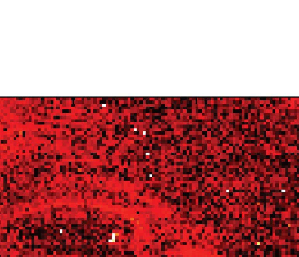
123

124 Chapter 4: Experimental Methods the contrast between the two liquids was lost due to the equal amount of elastic light scattered. Figure 4.20 shows a linescan of both the Brillouin frequency shift and the spectral linewidth measured along the interface between oil and water. The measured Bril ν B (GHz) Oil Water ν B (GHz) Oil Water x (µm) x (µm) Figure 4.20: 1D spatial distribution of the frequency shift (left) and the linewidth (right) of the Brillouin peaks along the two-liquid interface. louin frequency shift was B =(7.09 ± 0.11) GHz for water and B =(10.85 ± 0.13) GHz for oil, which gave an acoustic velocity of V water = ± 8.4 m/sand V oil = ± 9.6 m/srespectively. Thesevaluesshowedgoodagreementwith previous reports [47]. Experimental values for the spectral linewidth were B = (1.88 ± 0.23) GHz for water and B =(3.29 ± 0.32) GHz for oil, which showed an order-of-magnitude broadening with respect with previous analyses [47]. This is mainly caused by the instrumental broadening which a ects the peak linewidth even at low NA, as illustrated in Section 4.2. To summarise, a dark-field optical arrangement was employed as a suitable method to minimise undesired specular reflections. An annular beam was generated by means of a customised prism to illuminate the sample. The next step was to investigate the aspect ratio of the annulus that optimised the system performance. The beam size at the prism giving the highest throughput e ciency was estimated. The imaging system was first tested with an arbitrary sample to ensure minimal collection of surface reflections. Next, preliminary Brillouin images were acquired mainly using liquid interfaces. Overall, the microscope showed a good performance even though the data acqui- 124

125 4.5 Confocal Brillouin Microscopy sition time was relatively long. This represented the major instrumental limitation since a shorter integration period was required for the microscope to address real biological applications. 4.5 Confocal Brillouin Microscopy The annular illumination used in the Brillouin dark-field microscope was an e cient method to optically minimise collection of surface reflections allowing the isolated scattered radiation to be detected. This was particularly important when employing a single-stage VIPA spectrometer limited by an extinction ratio of roughly 30 db. Although the intensity of the system PSF was maximised through an appropriate choice of the annular beam size with respect to the aperture radius, the integration time required to acquire a single Brillouin spectrum of liquids was longer than one second. Since most unfixed biological samples have a limited lifetime before a change in their mechanical properties occurs, a decrease of at least one order of magnitude in the acquisition times was necessary. Besides the weak scattering signal at detection, the dark-field arrangement also su ered from an elongated longitudinal intensity distribution, as shown in Figure Inordertoovercometheselimits, afull scanning confocal system was built on the microscope. The following section describes the principles of a scanning confocal imaging system and the final optical arrangement used for fast high spatial resolution Brillouin microscopy Principles of Confocal Imaging A confocal microscope, first proposed by Nipkow and then designed by Minsky in 1957 to image high density neuronal tissues [158], is an optical microscope that uses a spatial filter to suppress the out-of-focus light collected from the sample [159, 160]. Light emitted by a point source is detected by a point detector, as shown in Figure An intermediate plane conjugate to the sample plane is used to spatially filter the light emitted from any other point objects in space. A spatial filter consists of a pinhole whose diameter is typically set to be equal to the width size of the central intensity distribution formed at the intermediate plane. For a 125

126

127 4.5 Confocal Brillouin Microscopy Dark Field Confocal Dark Field Confocal I(r,0) I(0,z) r (µm) z (µm) Figure 4.22: Transverse (left) and longitudinal (right) intensity distributions of a confocal imaging system characterised by a plane wave (red) and an annular dark-field (blue) illumination. dark-field arrangement is 25% narrower than that of the confocal system. On the other hand, the longitudinal intensity profile results to be 50% broader than that given by a confocal system uniformly illuminated, as shown in the right hand side of Figure The higher the NA at illumination of a confocal imaging system, the smaller the scattering volume. In highly heterogeneous samples, such as biological specimens, a small probe volume results in weak elastic signals due to smoother refractive index variations experienced by the beam in that sample volume [162, 163] Confocal Optical Setup Figure 4.23 shows the final confocal arrangement used to perform fast high spatial resolution Brillouin imaging. The objective lens is illuminated by a collimated Gaussian beam emitted by the single longitudinal mode laser ( = 561nm). Ahalfwave plate ( /2) placed at the laser output allowed rotation of the linear polarisation state of the input field. The beam was first expanded by a factor of 10 to fill the aperture of the microscope objective. Half of the input optical power was delivered to the objective lens by means of a 50/50 beam splitter (BS), which resulted in a higher throughput e ciency with respect to the dark-field setup. In order to minimise surface reflections at the sample plane and simultaneously increase the spatial 127

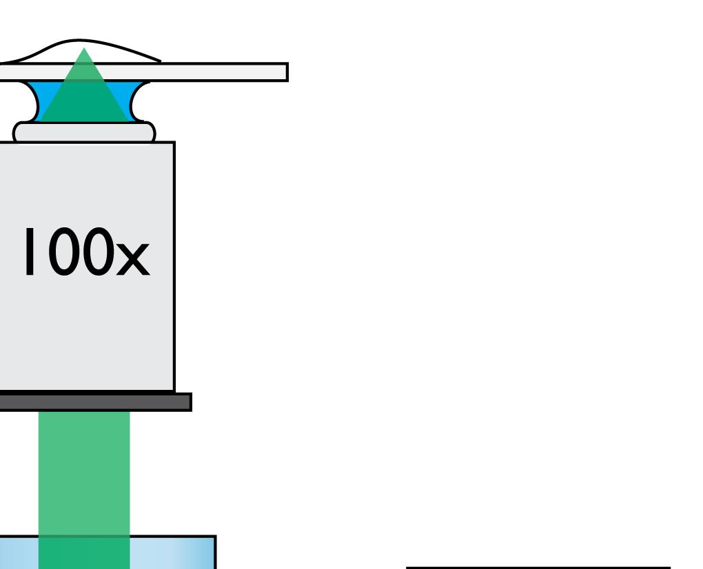
128

129 4.5 Confocal Brillouin Microscopy as to enhance the visibility of the Brillouin peaks detected by the scmos camera. Consequently, since the location of the elastic peaks could not be taken as a reference for the measurement of the frequency shift, another approach was taken. Specifically, the laser beam transmitted through the BS was focused into the glass cuvette filled with distilled water, which was used as a new reference signal. Before proceeding with the scanning of the sample, the system was calibrated with one frame acquisition of the Brillouin spectrum of water. This was taken by blocking the illumination arm of the inverted microscope in order to avoid detection of light coming from the sample. Water has a well known bulk modulus of B =2.2 GPa [25, 83, 164] whichmadeitsuitabletouseasaspectralreference.inthebackscattering geometry this gives a Brillouin frequency shift of B =7.04 GHz. This value was taken as a reference to measure the frequency shift of the Brillouin spectra acquired at each sampling point across the samples. The confocal arrangement described was ultimately employed to acquire mechanical images of several biological samples such as tissues and cells. 129

130 Chapter 4: Experimental Methods 130

131 Chapter 5 High Resolution Brillouin Imaging The confocal Brillouin microscope was used to investigate two di erent biological problems: on the one hand the sti ness variations in specific endothelium cells of the eye, aiming at a better understanding of the mechanisms responsible for glaucoma, and on the other the characterisation of the mechanical structures of blood vessels, which could provide fundamental information regarding the formation of atherosclerotic plaques. In this chapter, these results are presented. The Brillouin modulus of both PDMS gels and silicon rubber sheets of di erent sti nesses was measured. Correlation plots suggest the existence of a linear relationship between the Brillouin modulus and the standard Young s modulus, thus validating the technique as a reliable method for measuring sti ness. To the best of our knowledge this thesis presents, for the first time, sub-cellular Brillouin microscope images. Specifically, sti ness images of single Human Umbilical Vein Endothelial Cells (HUVEC) cells and blood vessel cross sections were acquired. These results may establish confocal Brillouin microscopy as the tool of choice for artery wall measurements, in particular when atherosclerotic plaques are formed. 131

132 Chapter 5: High Resolution Brillouin Imaging 5.1 Young s Modulus Correlation Before proceeding with the investigation of the mechanical properties that regulate biological systems, a validation of the technique as a reliable method to measure sti ness was necessary. As mentioned in Section 2.5, previousstudieshavefoundthebrillouinmodulus to be linearly related with the standard Young s modulus [54]. In order to provide an independent proof of this dependency and thus demonstrate that the Brillouin modulus is related to the material sti ness, several measurements were taken with the confocal system described in Section 4.5. In particular, both PDMS gels and semitransparent silicon rubber sheets were tested. PDMS gels were in-house made by Dr Sietse Braakman with sti ness varying from 5 kpa to 60 kpa. A standard uniaxial rheometer was used to measure the Young s modulus of the gels. This device measures the shear force using a load cell applied to the sample under test. Silicone rubber sheets were provided by Silex Ltd with a known Young s modulus ranging E =(1 6) MPa. Figure 5.1 shows the correlation plots between Brillouin modulus and Young s modulus. The Brillouin modulus was measured 10 times for each sample with an Brillouin Modulus (GPa) PDMS Brillouin Modulus (GPa) Silicone Rubber Young s Modulus (kpa) Young s Modulus (MPa) Figure 5.1: Measured Brillouin modulus as a function of the Young s modulus for PDMS gels (left) and silicon rubber sheets (right). The fits suggest that the two moduli are linearly correlated. However, the results show that the linear relationship varies depending on the material. exposure time of 1 second. The least-squares fits suggest the existence of a lin- 132

133 5.2 Cell Mechanics in Glaucoma ear relationship between Brillouin modulus and Young s modulus, which endorses Brillouin spectroscopy as a reliable method to measure sti ness. Although a linear correlation holds for both PDMS gels and silicone rubber sheets, the results show that this varies depending on the material properties, and ultimately represents a fundamental aspect that needs further investigation. 5.2 Cell Mechanics in Glaucoma Glaucoma is an asymptomatic eye disease a ecting about 60 million people worldwide. A late diagnosis of the disease can bring irreversible damages such as low vision and blindness. Glaucoma is typically associated with elevated intraocular pressure (IOP), which refers to the fluid pressure inside the eye. Currently, there is little understanding of why IOP becomes elevated in glaucoma or how to best reduce it to preserve vision. Recent studies have focused on the endothelial cells lining Schlemm s canal (SC), which serves as a collection vessel for aqueous humour drainage from the eye. The resistance of this drainage is increased in glaucoma and determines IOP [165]. Consequently, understanding the mechanism of this resistance generation lies at the heart of understanding and treating the disease. The key data are: SC cells are mechanosensitive, and form micron-sized pores (openings through the endothelial monolayer) in response to mechanical load. This is important because these pores provide a pathway for flow to enter the SC, where the mechanical loads in vivo are regulated by the pressure gradient arising from aqueous humour drainage. The SC endothelium therefore acts as a biomechanically regulated filtration barrier. glaucomatous SC cells form fewer pores than normal SC cells. This was directly observed in glaucomatous eyes by means of a novel cell culture model that mimics the SC barrier dysfunction in glaucoma [11]. recent AFM measurements have shown that glaucomatous Schlemm s canal cells are sti er than normal cells by approximately 50%. Nevertheless, AFM is primarily sensitive to cortical sti ness rather than to cytoplasmic sti ness, 133

134 Chapter 5: High Resolution Brillouin Imaging which appears elevated in glaucoma [166]. The cytoplasmic sti ness can only be measured indirectly by comparing the AFM data to multi-phase FE models of the cell. Confirming these findings using an independent and non-invasive method would be of great interest. In the following section, high resolution Brillouin images of single HUVEC cells are presented. Preliminary analyses have demonstrated that Brillouin microscopy has the potential to support the AFM data by directly measuring di erences in the cytoplasmic sti ness between normal and glaucomatous SC cells. Hitherto we have proved that when Latrunculin-A drug is applied directly to the endothelial cells, the sti ness decreases as suggested by previous AFM analyses [166, 167]. The results encourage further investigations on cell mechanics for a better understanding of the mechanisms that lead to glaucoma Cell Culture HUVEC cells stem from the endothelium of veins in the umbilical cord and are commonly used in pathological practises to investigate the origin of diseases derived from the endothelial layer. These were considered suitable for preliminary in vitro mechanical imaging. The cells were cultured by Dr Sietse Braakman in a dish filled with phosphate bu ered saline (PBS) solution, which is a water-based salt solution that is isotonic and non-toxic to cells and has the ability to maintain their osmolarity. The Brillouin modulus of PBS was measured to be M 0 =2.91 ± 0.14 GPa, which is comparable to that of water (M 0 ' 2.2 GPa). The HUVEC cells were deposited on a thin gelatin film (9% w/v) placed on top of the glass coverslip, as illustrated in Figure 5.2. A gelatin film of n ' 1.38 was used to yield a smoother variation in the refractive index across the interface that divides the glass coverslip (n ' 1.5) and the cells, which were assumed to have the same refractive index as water (n ' 1.33) [168, 169]. The larger the di erence in the refractive indexes at the sample interface, the higher the amount of optical reflections arising at that plane. Since the thickness of the human cells is typically afewmicrons[170, 171, 172], which is of the order of magnitude of the microscope depth of field, the gelatin film was necessary to prevent formation of strong crosstalk at the sample plane. 134

135

136 Chapter 5: High Resolution Brillouin Imaging Figure 5.3: Brillouin image of a single HUVEC cell. Both the nucleus membrane and the four nucleoli can be identified and appear to have a higher sti ness than the surrounding cytoplasm. content was ensured to be optically probed and spatially mapped. A water density of =1000Kg/m 3 was used when measuring the Brillouin modulus through equation Figure 5.4 shows the associated phase contrast image acquired with the same specimen. Phase contrast imaging is a dark-field modality that benefits from the retardation of light due to the spatial variations of the refractive index in the sample and is used to enhance the contrast of transparent specimens [174]. The image was acquired in a single frame using the Pulnix CCD camera mounted on a side port of the inverted Olympus microscope, which was set in the standard phase contrast mode. The Brillouin image showed great contrast between the cell and the surrounding PBS bu er solution. This contrast was lost in the associated phase contrast image due to a uniform spatial distribution of the refractive index. The elliptical shape of the cell nucleus could be clearly identified suggesting a higher sti ness for the nucleus membrane. Interestingly, the four nucleoli inside the cell nucleus appear 136

137 5.2 Cell Mechanics in Glaucoma Figure 5.4: Phase contrast image of the HUVEC cell. The sample was entirely illuminated by the microscope phase contrast mode and acquired by a Pulnix CCD camera. to be significantly sti er compared to the surrounding cytoplasm, which might be due to their high RNA content [175]. The Brillouin modulus was measured to be M 0 =3.03 ± 0.12 GPa for the nucleoli and M 0 =2.73 ± 0.24 GPa for the cytoplasm. Values of the Brillouin modulus were estimated by averaging over several regions of interest across the image Latrunculin-A for Sti ness Assessment Asetofmeasurementswastakentoinvestigatethee ectofthelatrunculin-a drug on the cell sti ness. Previous AFM measurements have reported a decrease in the Young s modulus in both HUVEC and SC cells when the drug was applied [166]. Specifically, the analyses showed that Latrunculin-A led to a decrease in the Young s modulus from E =1.40 ± 0.33 kpa to E =0.78 ± 0.26 kpa. The measurement was repeated using Brillouin microscopy. Figure 5.5 shows Brillouin images of the same HUVEC cell before and after the application of the drug. Cells were cultured in an equal process to that described in Section ThesampledisheswerefilledwithadilutedPBSsolution,whichwas sealed by a thin oil film so as to ensure thermal isolation. In order to decrease the 137

138 Chapter 5: High Resolution Brillouin Imaging Figure 5.5: Brillouin images of a HUVEC cell before (left) and after (right) the addition of Latrunculin-A. The sti ness images were normalised to the modulus of PBS solution. A 4% decrease in sti ness was found after the drug addition. data acquisition times to avoid dramatic changes in the thermodynamical properties of the cells during acquisition, samples were scanned with 1 µm stepsizeacrossthe xy plane. The exposure time was set to 0.5 sec/frame yielding a total acquisition period of 10 minutes for a single Brillouin image. In order to test whether temperature fluctuations or other environmental factors were a ecting the mechanical properties of the cells, two sets of measurements were taken with a time interval of approximately 30 minutes between each other. The acquisitions confirmed a constant level of sti ness over time with an average Brillouin modulus across the cytoplasm of M 0 =2.57 ± 0.54 GPa. Subsequently, the Latrunculin-A at 1 µm wasappliedtothe HUVEC cells and a third acquisition was taken with equal exposure time and step size. The two images shown in Figure 5.5 were normalised to the Brillouin modulus of the diluted PBS solution, which was measured to be M 0 =2.226 ± GPa. The average over the cytoplasmic region of the cell gave a Brillouin modulus of M 0 =2.36 ± 0.51 GPa, which represents approximately an 8% decrease in sti ness with respect to the original state. This result confirmed the outcome reported by the AFM measurements. As previously described, the Brillouin modulus was found to have a linear relationship with the Young s modulus and small changes in the Brillouin modulus reflect variations in the Young s modulus on a larger scale, which may justify the greater variation in sti ness reported in the previous AFM analysis. 138

139

140 Chapter 5: High Resolution Brillouin Imaging cardiovascular diseases. MI stems from disruption in blood flow to the heart muscle caused by plaque ruptures. In fact, expulsion of plaque content activates a cascade of events that eventually lead to thrombosis and death. Currently the only available strategy to reduce mortality in CAD is prevention, which is accomplished by monitoring the grade of sti ness of the artery walls. Clinical practices for diagnosis of atherosclerosis are primarily based on radio frequency screenings and ultrasound echocardiograms [178, 179, 180], which are intrinsically limited by a poor spatial resolution. Pulse wave velocity (PWV) is another common method that measures arterial pulse wave velocity to investigate elasticity in vivo [181, 182]. PWV increases with sti ness and is governed by the Moens-Korteweg equation, which is expressed as [182] s Eh PWV = 2 R, (5.1) where E is the Young s modulus of the arterial wall, h is the wall thickness, R is the artery diameter at the end of the diastole, which is the blood refilling process of the heart, and is the blood density. The distance and the time travelled by the pulse is estimated along the aorta and PWV is measured by means of either a pressure-sensitive transducer or Doppler ultrasound. PMW can also be measured in anon-invasivemannerbymeansofmri[183]. Besides the high costs, non-invasive PWV requires strong magnetic fields, which makes this technique di cult to apply in clinical studies. Other methods, such as blood tests, chest X rays and tomographic scans, can only help pathologists to estimate the extent of the disease. For instance, OCT is an established imaging technique which provides structural information of biological systems. OCT relies on the low-coherence interference between the scattered light and a broadband illumination source [184]. OCT has seen extensive use in imaging of coronary arteries and, over the last few years, has achieved a spatial resolution of a few microns [185]. Despite structural information of biological systems, this technique cannot retrieve their sti ness properties. We have established that confocal Brillouin microscopy can be used to successfully image the sti ness variations in the walls of blood vessels to sub-cellular reso- 140

141 5.3 Arteries Mechanics in Atherosclerosis lution, hence is a potential candidate as the tool of choice for earlier stage diagnoses. In the following sections, we review the use of confocal Brillouin microscopy in artery wall sti ness measurement and present examples of Brillouin microscope images Sample Preparation Optical clearing refers to a range of chemical protocols that provide a significant enhancement of the transparency of biological tissues [186]. The high scattering of turbid biological tissues limits the penetration depth of the probe beam, therefore a ecting the reconstruction of three dimensional images from di erent focal depths. Optical transparency can be achieved by embedding the tissue with an appropriate bu er solution in the attempt to match the refractive index of the specimen. Over the last decade, several protocols have been developed to reduce scattering from biological samples [187, 188]. These enabled a deeper penetration and an improved imaging contrast of the inner structures of the tissues. Besides an increase in the beam penetration depth, optical clearing can be of great advantage in confocal Brillouin microscopy where a high amount of elastic scattered light arising at the sample surface may impede the detection of the Brillouin spectra. Particular attention was paid in selecting a suitable bu er solution that did not a ect the mechanical properties of the tissues. For instance, VEC- TASHIELD Hard Set mounting medium was first tested as a standard clearing agent. However, its use led to a gradual sti ening of the tissue over a period of time of about 24 hours, hence it was discarded for our purposes. The final solution employed consisted of pure glycerol of refractive index n =1.47 close to that of biological tissues, which has been estimated to be approximately n =1.46 in the visible [189]. The Brillouin frequency shift of glycerol in the backscattering geometry was measured b =15.51 ± 0.12 GHz, and assuming a density of 1.26 g/cm 3 [190] the Brillouin modulus was estimated to be M 0 =11.03 ± 0.21 GPa. Cross sections of mice arteries were cut with a thickness of approximately 10 µm. Frozen sections were embedded in glycerol solution and sandwiched between a microscope slide and a standard glass coverslip of thickness 170 µm. It must be noted that the glycerol solution did not penetrate the tissues but it was used as an immersion bu er to reduce the elastic scattering at the sample surface. Nail polish 141

142 Chapter 5: High Resolution Brillouin Imaging was used to seal the glass coverslip to avoid sample displacement and dehydration during acquisitions Artery Mechanical Imaging Before investigating the mechanical properties of the atherosclerotic plaques, several acquisitions were performed with normal mouse blood vessels. Figures 5.7 and 5.8 show the Brillouin image and the associated phase contrast image of an entire mouse artery cross section. The Brillouin image was taken with an exposure time of 0.35 Figure 5.7: Brillouin image of a cross section of a normal mouse blood vessel. The adventia appears to be sti er compared to the inner substrate, as suggested by morphological studies. sec/frame and a scan step of 1.2 µm. Data acquisition started approximately 30 minutes after sample preparation in order to allow the frozen tissue to stabilise at the room temperature ( 24 C). Total acquisition time required approximately 14 hours. As previously discussed, the reason why the scanning step size was greater than the optical resolution was purely due to time restrictions. The longer the data 142

143 5.3 Arteries Mechanics in Atherosclerosis acquisition time, the higher the risk of mechanical changes in the embedded tissue. Figure 5.8: Associated phase contrast image of the artery cross section. The blood vessel walls exhibited a significant spatial variation in sti ness, which could be directly observed in the Brillouin image. A significant di erence in the elastic modulus was found between the outer wall of the artery and the inner layers close to the lumen, which is the inside space of the tubular structure. The outer layer known as the adventia appears to be sti er than the inner structure. The Brillouin modulus was estimated by averaging over di erent regions of interest across the image, yielding M 0 = ± 0.27 GPa for the outside tissue and M 0 = ± 0.31 GPa for the inside layer. These results confirm the current understanding of a higher sti ness corresponding to the outside of blood vessels than that of the inside. In fact, morphological studies have assessed the adventia formed by a strong fibrous tissue which maintains the vessel shape in a robust shell [191, 192]. On the other hand, the inner structure is divided by the tunica media and the tunica intima. These are composed of smooth muscles, elastic lamina and connective tissues containing high amounts of lipids. The assumption of a softer arterial inner substrate stems from the high concentration of lips, which are mostly composed of fat molecules [193]. Nevertheless, no direct evidence of this property has been found in arteries. To the best of our knowledge, the results obtained with the confocal Brillouin microscope 143

144 Chapter 5: High Resolution Brillouin Imaging represent the first quantitative proof of this hypothesis. As previously discussed, other conventional elastography techniques are limited by a lower spatial resolution, which impedes distinguishing the outer from the inner regions. Figure 5.9 shows the sti ness image corresponding to a small region of a mouse artery cross section. In order to obtain a more detailed structure of the wall sti ness, Figure 5.9: High resolution Brillouin image of a small region of a normal artery cross section. The image confirms a higher sti ness for the adventia. Interestingly, layers of di erent elasticities can be identified within the tunica wall. the scan step was decreased to 0.4 µm, which was close to the full transverse resolution of the microscope (r =0.26 µm). Integration time was set to 0.3 sec/frame for a total acquisition period of approximately 1 hour. The image confirmed a higher Brillouin modulus for the adventia. Interestingly, thin layers of di erent sti nesses can be identified along both the tunica media and the tunica intima of the artery. This suggests that normal arteries might be formed by more complex structures than that evinced from morphological studies. The endothelium substrate next to the lumen appears to be sti er than the tunica intima. Overall, the Brillouin modulus of the artery can be observed to lie within the range M 0 =10 14 GPa, which is significantly higher with respect to that of the HUVEC cells previously investigated (M 0 = GPa). 144

145 5.3 Arteries Mechanics in Atherosclerosis Mechanical Imaging of Atherosclerotic Plaques The results obtained with normal blood vessels encouraged the application of the Brillouin microscope to the investigation of the mechanical properties of atherosclerotic plaques. Measurements were taken for both healthy and diseased mouse blood vessels. Female ApoE-/- mice (20-23 grams in weight) were used for all biological experiments, which were conducted by Dr Ryan Pedrigi. The artificial growth of atherosclerotic plaques in the animals was driven using a similar procedure to that applied by Cheng et al. [194, 195]. In particular, the mice were placed on a high-fat Western-type diet (Lillico Biotech, UK) at the age of 11 weeks. Two weeks later, the mice went through the surgical procedure of placing a flow-modifying cu on the left carotid arteries. The cu was composed of two thermoplastic polyetherketone cylindrical halves with a conical lumen that tapers from 500 µm at the base to 250 µm at the throat of the cu. The placement of the cu creates a gradual stenosis in the artery, leading to shear stress-related plaque initiation. Atherosclerotic lesions developed in the vicinity of the chu base where shear stress was lower. Successively, 30 cross sections were exported from both a diseased and a healthy (test) artery of the same mouse. Each section addressed to Brillouin imaging was accompanied by an adjacent slice, which underwent to an Oil-red-O staining process [196] to highlight the region of the artery with high lipid concentration. Brillouin images of 15 cross sections of both healthy and diseased arteries were acquired for sti ness measurement. Figure 5.10 shows thesti ness imageof onecross section of the diseased artery. The image was taken with an exposure time of 0.3 sec/frame and a scan step of 1.8 µm foratotalacquisitionperiodofapproximately 14 hours. The associated phase contrast and stained images are shown in Figure Theregionofhighlipidcontentofthetissuewasmarkedinredcolourfollowing the Oil-red-O staining (0.5% Oil-red-O solution in Propylene glycol) with Mayers Hemotoxylin counterstain. Since the atherosclerotic lesion is associated with a high lipid accumulation, this plaque region could be identified in the stained image. The outer annular wall of the artery was found to be sti er than the atheromatous plaque, as shown in Figure In this case, however, the adventia and the inner 145

146 Chapter 5: High Resolution Brillouin Imaging Figure 5.10: Cross sectional Brillouin image of a mouse blood vessel a ected by atherosclerosis. The outer tissue appear to be sti er with respect to the plaque. The image suggests that the plaque is formed of a variety of organic materials of di erent sti nesses. tunica of the artery wall appeared more uniform in sti ness with respect to the healthy vessels shown in Figure 5.7 and 5.9. TheBrillouinmodulusinthediseased wall region was estimated to be M 0 =12.64 ± 0.33 GPa. On the other hand, it was observed that the atherosclerotic plaque was composed of a complex mixture of organic compounds with di erent elasticity. Unlike the stained sections, Brillouin images suggest an accumulation of softer materials in the narrow region surrounding the lumen. The Brillouin modulus of the atheromatous plaque was found to be M 0 =9.72 ± 0.36 GPa in the vicinity of the lumen and M 0 =11.36 ± 0.45 GPa in the central region of the plaque. In order to obtain a more quantitative figure, Brillouin images of diseased and 146

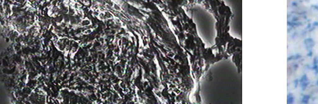
147