MATLAB for Chemical Engineering

Transcription

1 MATLAB for Chemical Engineering Dr. M. Subramanian Associate Professor Department of Chemical Engineering Sri Sivasubramaniya Nadar College of Engineering OMR, Chennai msubbu.in[at]gmail.com 16 th March 2012

2 Contents I. Mathematical Models in Chemical Engineering II. Getting Started with MATLAB III. MATLAB examples for Solving typical ChE problems IV. Getting Started with Simulink

3 Part I Mathematical Models in Chemical Engineering

4 Modeling & Simulation

5 Types of Mathematical Models Mathematical models are of two types: based on physical theory empirical Models based on physical theory can be further divided into the following categories: Linear / non-linear Steady / unsteady Lumped / distributed parameter system Continuous / discrete variables

6 Forms of Mathematical Models Algebraic equations Linear nonlinear Integral equations Differential equations Ordinary differential Partial differential Difference equations

7 Chemical Industry Problems

8

9 Basis of Mathematical Models in Chemical Engineering Laws of physics, chemistry, such as conservation of mass, energy, and momentum Equation of state Equilibrium relationships Rate laws

10 Mathematical Problems in Chemical Engineering Linear algebraic equations Non-linear equations Curve fitting polynomial, non-linear Interpolation Integration Differential equations Partial differential equations

11 Part II Getting Started with MATLAB

12 About MATLAB MATLAB has become a standard among academic and industrial users Developed by Math Works Inc. MATLAB -acronym for MATrix LABoratory Matrices and arrays -the heart of MATLAB Offers programming features -similar to other languages

13 Capabilities of MATLAB Provides extensive numerical resources Contains lot of reliable, accurate mathematical subprograms The subprograms provide solutions to broad range of mathematical problems including: matrix algebra, complex arithmetic, differential equations, nonlinear systems, and many special functions Provides a variety of graphic output displays: linear, log-log, semilog, polar, bar chart, and contour plots 2-D and 3-D views Provides GUI tool: Simulink block diagram representation, simulation

14 Workspace Window Command Window Command History Window

15

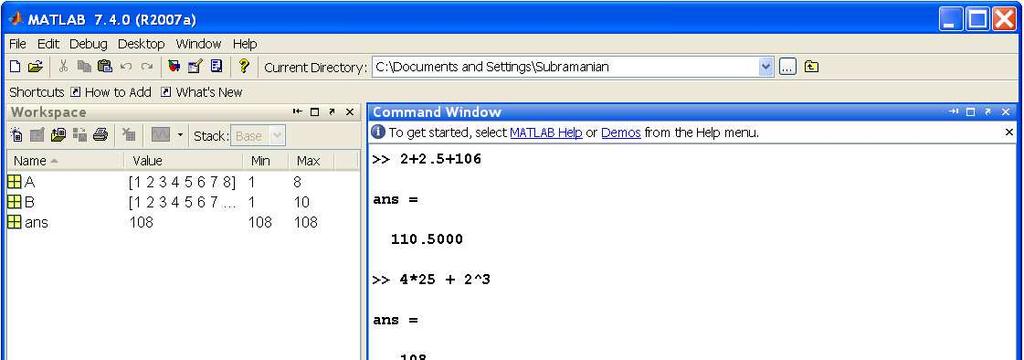
16 MATLAB Variables» D = 2 D = 2 ans pi Default variable name used for resuts Value of π» v = 3 v = 3» rho = 1000;» mu = 0.001;» Re = D*v*rho/mu Re =» inf Stands for infinity (e.g., 1/0) NaN Stands for Not-a-Number (e.g., 0/0) i, j i = j = -1» c1 = 2+3i c1 = i

17 Mathematical Functions» x=sqrt(2)/2 x = » y=sin(x) y = Trigonometric functions Exponential functions sin, cos, tan, sin, acos, atan, sinh, cosh, tanh, asinh, acosh, atanh, csc, sec, cot, acsc, exp, log, log10, sqrt Complex functions abs, angle, imag, real, conj» Rounding and Remainder functions floor, ceil, round, mod, rem, sign

18 Array Operations» x = 1:10;» y = sin(x) y = Columns 1 through Columns 8 through » y(3) ans = » y(1:5) ans =

19 » A = [1 2; 3 4; 5 6] A = Array Manipulation» A+B??? Error using ==> plus Matrix dimensions must agree » B = [1 2 3; 4 5 6];»» A*B ans =» A' ans = »

20 Element by Element Operation» clear» a = [1 2; 3 4];» b = [1 1; 2 2];»» a.*b ans =» » a./b ans = » a/b Warning: Matrix is singular to working precision. ans = -Inf Inf -Inf Inf»

21 » A = [1 2; 3 4];» B = [1 1; 2 2]; Matrix Operations» C = [A B] C =» [A B] ans =» ans-1 ans = » C(1,:) ans = » C(:,2:end) ans =

22 Matrix Functions» A A =» det(a) ans = -2» inv(a) ans = »» [a b] = eig(a) a = b =» Related: diag, triu, tril, rank, size

23 Using Script M-files» frictionfactor Dia in meter =.1 Velocity in m/s = 2 Re = »

24 Control Flow Statements for <index=start:end> end if <expression> else end while <condition> end switch expression end case option1 case option2. case optionn otherwise

25 Part III Capabilities of MATLAB in Solving Typical Chemical Engineering Problems

26 Matrix Problems To calculate the quantities of each of the three acids required for making 100 kg blended acid: Component Compositions of acids Composition Spent acid Aqueous HNO 3 Y Aqueous H 2 SO 4 Z of blended acid X H 2 SO HNO H 2 O H 2 SO 4 balance: 44.4 X + 0 Y + 98 Z = 60 HNO 3 balance: 11.3 X + 90 Y + 0 Z = 32 H 2 O balance: 44.3 X + 10 Y + 2 Z = 8» A = [ ]» B = [ ]» x = inv(a)*b x = Similar Problems: Stage by stage calculations of absorber, extractor, with linear equilibrium relationships, under isothermal operation

27 Plots» x = 1:2:50;» y = x.^2;» plot(x,y,'*-')» xlabel('values of x')» ylabel('y')»» P = logspace(3,7);» Q = 0.079*P.^(-0.25);» loglog(p,q, '.-')» grid

28 Non-linear Equation % pvt_calculation.m global R T P Tc Pc T = input('temperature in K ') P = input('pressure in Bar ') R = ; % Bar.m3/kmol.K Tc = 190.6; % Tc of Methane K Pc = 45.99; % Pc of Methane bar v_ig = R*T/P v_vander = fzero('vander',v_ig) % % vander.m function v2 = vander(vol); global R T P Tc Pc a = 27*(R^2)*(Tc^2)/(64*Pc); b = R*Tc/(8*Pc); v2 = R*T - (P + a/vol^2)*(vol-b); % » pvt_calculation Temperature in K 350 Pressure in Bar 30 v_ig = v_vander = »

29 Non-linear Equations van Laar equations: Relates γ i with x i. Estimating the parameters (A 12, A 21 ) based on γ i, x i data, involves solving the nonlinear algebraic equations.

30 Solution to Non-linear Equations function Eqn = vanlaareqns(a, x1, g1, g2) % to solve for vanlaar parameters A1, A2 x2 = 1-x1; Eqn(1) = log(g1) - A(1)*(1+ (A(1)*x1/(A(2)*x2)))^(-2); Eqn(2) = log(g2) - A(2)*(1+ (A(2)*x2/(A(1)*x1)))^(-2); % end» x_1 = 0.561; g_1 = ; g_2 = ; Azero = [2 2];» Asolved = fsolve(@vanlaareqns, Azero, [], x_1, g_1, g_2) Optimization terminated: first-order optimality is less than options.tolfun. Asolved = »

31 Non-linear Equations in ChE Terminal settling velocity Pressure drop vs. velocity for flow through pipelines, Piping network calculations, pressure drop / velocity calculations in packed and fluidized beds PVT relations nonlinear algebraic Internal Rate of Return (IRR) calculations

32 V = ZRT/P Interpolations» interp2(pr_data,tr_data,z0_data,0.5,0.48) ans =

33 Polynomial Fitting» T=[0,18,25,100,200,300,400,500];» Cp=[8.371, 8.472, 8.514, 9.035, 9.824, , , ];» P=polyfit(T,Cp,3) P = C p = at 3 + bt 2 + ct + d» T_range = [0:500];» Cp_fit = P(1).*T_range.^3+P(2).*T_range.^2+P(3).*T_range+P(4);» plot(t,cp,'*',t_range,cp_fit)

34 % AntoineFit.m function AntoineFit % T in oc; P in kpa % ln P = A - B/(T+C) Nonlinear Curve Fitting ln P = A - B/(T+C) T = [ ]; P = [ ]; ABC0 = [ ]; % Starting guess

35 % AntoineFit.m contd.. ABCfit = lsqcurvefit(@eqnform,abc0,t,p) Tfit = [50:5:250]; Pfit = exp(abcfit(1) - ABCfit(2)./(Tfit + ABCfit(3))); plot(t,p,'+',tfit,pfit,'-') function Psat = EqnForm(ABC,Tdata) Psat = exp(abc(1) - ABC(2)./(Tdata + ABC(3))); % » AntoineFit ABCfit =

36 Nonlinear Curve Fitting in ChE Langmuir-Hinshelwood kinetics Parameters of Redlich-Kister expansion for property changes of mixing Activity coefficient-composition models

37 Ordinary Differential Equations To plot the variation in tank levels for two interacting tanks From mass balance, and using Bernoulli equations, we get:

38 Solving ODEs %twotnk.m function hdot = twotnk(t,h) % To solve % dh1/dt = 1-0.5*sqrt(h1-h2) % dh2/dt = 0.25*sqrt(h1-h2) *sqrt(h2) hdot = zeros(2,1); % a column vector hdot(1) = 1-0.5*sqrt(h(1)-h(2)); hdot(2) = 0.25*sqrt(h(1) - h(2)) *sqrt(h(2));» [t, h] = ode45(@twotnk, [0 100], [12 7]');» plot(t, h)

39 ODE Problems in ChE Reaction Engineering Concentration vs time (dc/dt), Heat Transfer Temperature vs time(dt/dt), Temperature vs distance (dt/dx)

40 Part IV Getting Started with Simulink

41 Simulink SIMULINKis an extension to MATLABwhich uses a icon-driven interface for the construction of a block diagram representation of a process. Inputs System Outputs Steps involved in Simulink Solution: Creating the Block Diagram Specifying the Block Parameters Setting up the Solver Running the Simulation

42 New Simulink File

43 Arranging the Blocks

44 Connecting the Blocks

45 Specifying Block Parameters

46 Running the Simulation

47 PID with Step Change in Set-point

48 Vapor Pressure from Antoine Equation

49 Bubble Pressure and Composition

50 Thank You!