ENVIRONMENTAL ADAPTIVE SAMPLING FOR MOBILE SENSOR NETWORKS USING GAUSSIAN PROCESSES. Yunfei Xu

Transcription

1 ENVIRONMENTAL ADAPTIVE SAMPLING FOR MOBILE SENSOR NETWORKS USING GAUSSIAN PROCESSES By Yunfei Xu A DISSERTATION Submitted to Michigan State University in partial fulfillment of the requirements for the degree of DOCTOR OF PHILOSOPHY Mechanical Engineering 2011

2 ABSTRACT ENVIRONMENTAL ADAPTIVE SAMPLING FOR MOBILE SENSOR NETWORKS USING GAUSSIAN PROCESSES By Yunfei Xu In recent years, due to significant progress in sensing, communication, and embedded-system technologies, mobile sensor networks have been exploited in monitoring and predicting environmental fields (e.g., temperature, salinity, ph, or biomass of harmful algal blooms). The conventional inverse problem approach based on physical transport models is computationally prohibitive for resource-constrained, multi-agent systems. In contrast, emphasizing practicality and usefulness, this work relies extensively on the phenomenological and statistical modeling techniques, in particular, Gaussian processes. However, such statistical models need to be carefully tailored such that they can be practical and usable for mobile sensor networks with limited resources. In this dissertation, we consider the problem of using mobile sensor networks to estimate and predict environmental fields modeled by spatio-temporal Gaussian processes. In the first part of the dissertation, we first present robotic sensors that learn a spatiotemporal Gaussian process and move in order to improve the quality of the estimated covariance function. For a given covariance function, we then theoretically justify the usage of truncated observations for Gaussian process regression for mobile sensor networks with limited resources. We propose both centralized and distributed navigation strategies for resource-limited mobile sensing agents to move in order to reduce prediction error variances at points of interest. Next, we formulate a fully Bayesian approach for spatio-temporal Gaussian process regression such that multifactorial effects of observations, measurement

3 noise, and prior distributions of hyperparameters are all correctly incorporated in the posterior predictive distribution. To cope with computational complexity, we design sequential Bayesian prediction algorithms in which exact predictive distributions can be computed in constant time as the number of observations increases. Under this formulation, we provide an adaptive sampling strategy for mobile sensors, using the maximum a posteriori (MAP) estimation to minimize the prediction error variances. In the second part of the dissertation, we address the issue of computational complexity by exploiting the sparsity of the precision matrix used in a Gaussian Markov random field (GMRF). The main advantages of using GMRFs are: (1) the computational efficiency due to the sparse structure of the precision matrix, and (2) the scalability as the number of measurements increases. We first propose a new class of Gaussian processes that builds on a GMRF with respect to a proximity graph over the surveillance region, and provide scalable inference algorithms to compute predictive statistics. We then consider a discretized spatial field that is modeled by a GMRF with unknown hyperparameters. From a Bayesian perspective, we design a sequential prediction algorithm to exactly compute the predictive inference of the random field. An adaptive sampling strategy is also designed for mobile sensing agents to find the most informative locations in taking future measurements in order to minimize the prediction error and the uncertainty in the estimated hyperparameters simultaneously.

4 ACKNOWLEDGMENT I would like to thank everybody who helped to accomplish this dissertation. First of all, I would like to express my sincere appreciation and gratitude to my advisor, Dr. Jongeun Choi, who continuously encouraged, and supported me. This thesis is not possible without his invaluable advice and effort to improve the work. In addition, I would like to thank all my committee members, Dr. Ranjan Mukherjee, Dr. Xiaobo Tan, Dr. Guoming Zhu, and Dr. Tapabrata Maiti, for their contribution and suggestions. I would also like to thank my colleagues, Mr. Mahdi Jadaliha and Mr. Justin Mrkva, for their help to obtain experimental data. Last but not least, I cannot thank enough my parents and my wife for always being there for me. I would never have been able to accomplish what I have without them. iv

5 TABLE OF CONTENTS List of Tables viii List of Figures ix 1 Introduction Background Contribution Organization Publication Journal Articles Conference Proceedings Preliminaries Mathematical Notation Physical Process Model Gaussian process Spatio-temporal Gaussian process Gaussian Markov random field Mobile Sensor Network Gaussian Processes for Regression Learning the Covariance Function Learning the Hyperparameters Optimal Sampling Strategy Simulation Spatio-temporal Gaussian process Time-varying covariance functions Advection-diffusion process Prediction with Known Covariance Function GPR with Truncated Observations Error bounds in using truncated observations Selecting temporal truncation size Optimal Sampling Strategies Centralized navigation strategy Distributed navigation strategy Simulation v

6 4.3.1 Gradient-based algorithm vs. exhaustive search algorithm Centralized sampling scheme Distributed sampling scheme Fully Bayesian Approach Fully Bayesian Prediction Approach Prior selection MCMC-based approach Importance sampling approach Discrete prior distribution Sequential Bayesian Prediction Scalable Bayesian prediction algorithm Distributed implementation for a special case Adaptive sampling Simulation MCMC-based approach on a 1-D scenario Centralized scheme on 1-D scenario Distributed scheme on 2-D scenario Gaussian Process with Built-in GMRF Spatial Prediction Spatial model based on GMRF Gaussian process regression Sequential prediction algorithm Distributed Spatial Prediction Distributed computation Distributed prediction algorithm Simulation and Experiment Simulation Centralized scheme Distributed scheme Experiment Bayesian Spatial Prediction Using GMRF Problem Setup Spatial field model Mobile sensor network Bayesian Predictive Inference Sequential Bayesian Inference Update full conditional distribution Update likelihood Update predictive distribution Adaptive Sampling Simulation vi

7 8 Conclusion and Future Work Conclusion Future Work A Mathematical Background 155 A.1 Gaussian Identities A.2 Matrix Inversion Lemma A.2.1 Woodbury identity A.2.2 Sherman-Morrison formula A.3 Generating Gaussian processes A.3.1 Cholesky decomposition A.3.2 Circulant embedding Bibliography vii

8 LIST OF TABLES 3.1 Centralized optimal sampling strategy at time t Parameters used in simulation Prediction means and variances using y, y m, and y r Centralized sampling strategy at time t Distributed sampling strategy at time t Gibbs sampler Centralized Bayesian prediction algorithm Sequential algorithm for field prediction Distributed algorithm for sequential field prediction Sequential Bayesian predictive inference A.1 Generating multivariate Gaussian samples by Cholesky decomposition A.2 Generating multivariate Gaussian samples by circulant embedding viii

9 LIST OF FIGURES 2.1 Realization of a Gaussian process. For interpretation of the references to color in this and all other figures, the reader is referred to the electronic version of this dissertation Realization of Gaussian process at (a) t = 1, (b) t = 5, and (c) t = Snap shots of the realized Gaussian process at (a) t = 1, (b) t = 10, and (c) t = Monte Carlo simulation results (100 runs) for a spatio-temporal Gaussian process using (a) the random sampling strategy, and (b) the adaptive sampling strategy. The estimated hyperparameters are shown in blue circles with errorbars. The true hyperparameters that used for generating the process are shown in red dashed lines Predicted fields along with agents trajectories at (a) t = 1 and (b) t = (a) Weighting factor λ(t) and (b) the estimated λ(t) Snap shots of the advection-diffusion process at (a) t = 1 and (b) t = Simulation results (100 runs) for a advection-diffusion process. The estimated hyperparameters with (a) random sampling and (b) optimal sampling Robot predicts a scalar value at x (denoted by a red star) based on cumulative n spatio-temporal observations (denoted by blue crosses). Near-optimal prediction can be obtained using truncated observations, e.g., the last m observations. In this case, x = (s x, s y, t) T Example of the selection of truncated observations. The parameters used in the example are: σ 2 f = 1, σ l = 0.2, σ w = Example of selecting a temporal truncation size η. The parameters used in the example are: σ 2 f = 1, σ x = σ y = 0.2, σ t = 5, γ = ix

10 4.4 Function Φ(d) in (4.22) with γ = 100, R = 0.4, and d 0 = 0.1 is shown in a red dotted line. The function Φ(d) = γ is shown in a blue solid line Prediction error variances at t = 5 achieved by (a) using the gradient-based algorithm, and (b) using the exhaustive search algorithm. The trajectories of the agent are shown in solid lines Average of prediction error variances over target points (in blue circles) achieved by the centralized sampling scheme using all collective observations for (a) case 1, (b) case 2, and (c) case 3. In (a), the target points are fixed at time t = 10, and the counterpart achieved by the benchmark random sampling strategy is shown in red squares with error-bars. In (b) and (c), the target points are at t + 1 and change over time. The counterpart achieved by using truncated observations are shown in red squares Simulation results at t = 1 and t = 5 obtained by the centralized sampling scheme for case Simulation results at t = 1 and t = 5 obtained by the centralized sampling scheme for case 2 (cont d) Simulation results obtained by the centralized sampling scheme for case 3. The trajectories of agents are shown in solid lines Cost function J d ( q) from t = 1 to t = 2 with a communication range R = Average of prediction error variances over all target points and agents achieved by the distributed sampling scheme with a communication range (a) R = 0.3, and (b) R = 0.4. The average of prediction error variances over all target points and agents are shown in blue circles. The average of prediction error variance over local target points and agents are shown in red squares. The error-bars indicate the standard deviation among agents Simulation results obtained by the distributed sampling scheme with different communication ranges. The edges of the graph are shown in solid lines Simulation results obtained by the distributed sampling scheme with different communication ranges (cont d). The edges of the graph are shown in solid lines Example with three agents sampling the spatio-temporal Gaussian process in 1-D space and performing Bayesian inference. In this example, σ t = 2.5, η = 2, = 3, t = 15, c t = 2, ȳ = (y T 1:3, yt 6:8 )T and ỹ = y 13: x

11 5.2 Example with three group of agents sampling the spatio-temporal Gaussian process in 2-D space and performing Bayesian prediction. The symbol o denotes the position of a leader for a group and the symbol x denotes the position of an agent. Distance between any two sub-regions is enforced to be greater than σ s which enables the distributed Bayesian prediction Posterior distribution of β, σ 2 f, σ s, and σ t at (a) t = 1, and (b) t = Prediction at (a) t = 1, and (b) t = 20 using the MCMC-based approach. The true fields are plotted in blue solid lines. The predicted fields are plotted in red dash-dotted lines. The area between red dotted lines indicates the 95% confidence interval Prediction at t = 1 using (a) the maximum likelihood based approach, and (b) the proposed fully Bayesian approach. The true fields are plotted in blue solid lines. The predicted fields are plotted in red dash-dotted lines. The area between red dotted lines indicates the 95% confidence interval (a) Prior distribution θ, (b) posterior distribution of θ at time t = 100, (c) posterior distribution of θ at time t = Prediction at (a) t = 100, and (b) t = 300 using the centralized sequential Bayesian approach. The true fields are plotted in blue solid lines. The predicted fields are plotted in red dash-dotted lines. The area between red dotted lines indicates the 95% confidence interval Posterior distribution of θ at time t = 100 using the distributed algorithm Comparison of (a) the true field at t = 100 and (b) the predicted field at t = 100 using the distributed algorithm (a) Generating points in blue dots and the associated Delaunay graph with edges in red dotted lines. The Voronoi partition is also shown in blue solid lines. (b) Gaussian random field with a built-in GMRF with respect to the Delaunay graph in (a) Example of computing (Λ T Λ) ij = λ(s l, p i )λ(s l, p j ) Simulation results for the centralized scheme. (a) The true field, (b) the predicted field at time t = 1, (c) the predicted field at time t = 5, (d) the predicted field at time t = 20. The generating points are shown in black circles, and the sampling locations are shown in black crosses xi

12 6.4 (a) Graph G = (V, E). (b) Sparsity structure of the precision matrix Q Simulation results for the distributed scheme. (a) The true field, (b) the predicted field at time t = 5. The generating points are shown in circles, and the sampling locations are shown in crosses (a) True field on grid positions obtained by the Kinect sensor and randomly sampled positions indicated in black crosses. (b) The fitted Gaussian random field with a build-in GMRF with respect to the Delaunay graph Elements of the precision matrix Q related to a single location Numerically generated spatial fields defined in (7.1) with µ(s i ) = β = 20, and Q η θ constructed using (7.2) with hyperparameters being (a) θ = (4, ) T, (b) θ = (1, 0.01) T, and (c) θ = (0.25, 0.04) T Posterior distributions of θ, i.e., π(θ y 1:t ), at (a) t = 1, (b) t = 5, (c) t = 10, and (d) t = Predicted fields at (a) t = 1, (c) t = 5, (e) t = 10, and (g) t = 20. Prediction error variances at (b) t = 1, (d) t = 5, (f) t = 10, and (h) t = Predicted fields at (a) t = 1, (c) t = 5, (e) t = 10, and (g) t = 20. Prediction error variances at (b) t = 1, (d) t = 5, (f) t = 10, and (h) t = 20 (cont d) (a) Estimated β, and (b) root mean square error xii

13 Chapter 1 Introduction In recent years, due to drastic global climate changes, it is necessary to monitor the changing ecosystems over vast regions in lands, oceans, and lakes. For instance, for certain environmental conditions, rapidly reproducing harmful algal blooms in the lakes can cause the death of nearby fish and produce harmful conditions to aquatic life as well as human beings 1. Besides natural disasters, there exist growing ubiquitous possibilities of the release of toxic chemicals and contaminants in the air, lakes, and public water systems. Hence, there are strong motivations to monitor and predict the environmental field undergoing often complex transport phenomena 2. In this dissertation, we consider the problem of using mobile sensor networks to estimate and predict environmental fields that are modeled by spatio-temporal Gaussian processes. 1 See for more details. 2 Common examples are diffusion, convection, and advection. 1

14 1.1 Background Due to the recent advances of micro-electro-mechanical systems technology, wireless communications and digital electronics, the concept of sensor networks has been made viable [2]. A sensor network consists of a collection of low-cost, low-power, multifunctional sensing devices that are small in size and communicate in short distances. Endowing the nodes in a sensor network with mobility increases the network s capabilities drastically [7]. The sensor networks which consist of mobile sensing agents are more flexible than the ones with only static nodes. For example, the mobility allows the network to handle a large number of data sources with a much smaller number of moving sensors that visit the sources over time. In a mobile sensor network, the resource limited sensing agents are required to collaborate in order to meet a specific objective. The cooperative control becomes essential. The most popular applications are in networks of autonomous ground vehicles, underwater vehicles, or aerial vehicles. Emerging technologies have been reported on the coordination of mobile sensing agents [28,37,46,52,68,69]. The mobility of mobile agents can be designed in order to perform the optimal sampling of the field of interest. Optimal sampling design is the process of choosing where to take samples in order to maximize the information gained. Recently in [35], Leonard et al. developed mobile sensor networks that optimize ocean sampling performance defined in terms of uncertainty in a model estimate of a sampled field. However, this approach optimized the collective patterns of mobile agents parameterized by a restricted number of parameters rather than optimizing individual trajectories. In [10], distributed learning and cooperative control were developed for multi-agent systems to discover peaks of the unknown field based on the recursive estimation of an unknown field. A typical sensor placement technique [16] that puts sensors at the locations where the entropy is high 2

15 tends to place sensors along the borders of the area of interest [32]. In [32], Krause et al. showed that seeking sensor placements that are most informative about unsensed locations is NP-hard, and they presented a polynomial time approximation algorithm by exploiting the submodularity of mutual information [14]. In a similar approach, in [58], Singh et al. presented an efficient planning of informative paths for multiple robots that maximizes the mutual information. To find these locations that predict the phenomenon best, one needs a model of the spatiotemporal phenomenon. To this end, we use the Gaussian processes (Gaussian random fields) to model fields undergoing transport phenomena. Nonparametric Gaussian process regression (or Kriging in geostatistics) has been widely used as a nonlinear regression technique to estimate and predict geostatistical data [15,23,38,51]. A Gaussian process is a natural generalization of the Gaussian probability distribution. It generalizes a Gaussian distribution with a finite number of random variables to a Gaussian process with an infinite number of random variables in the surveillance region [51]. Gaussian process modeling enables us to predict physical values, such as temperature, salinity, ph, or biomass of harmful algal blooms, at any point with a predicted uncertainty level efficiently. For instance, near-optimal static sensor placements with a mutual information criterion in Gaussian processes were proposed in [31, 32]. A distributed Kriged Kalman filter for spatial estimation based on mobile sensor networks is developed in [13]. Multi-agent systems that are versatile for various tasks by exploiting predictive posterior statistics of Gaussian processes were developed in [9] and [8]. However, Gaussian process regression, based on the standard mean and covariance functions, requires an inversion of a covariance matrix whose size grows as the number of observations increases. 3

16 The advantage of a fully Bayesian approach is that the uncertainty in the model parameters are incorporated in the prediction [5]. In [22], Gaudard et al. presented a Bayesian method that uses importance sampling for analyzing spatial data sampled from a Gaussian random field whose covariance function was unknown. However, the solution often requires Markov Chain Monte Carlo (MCMC) methods, which greatly increases the computational complexity. In [25], an iterative prediction algorithm without resorting to MCMC methods has been developed based on analytical closed-form solutions from results in [22], by assuming that the covariance function of the spatio-temporal Gaussian random field is known up to a constant. Recently, there have been efforts to find a way to fit a computationally efficient Gaussian Markov random field (GMRF) on a discrete lattice to a Gaussian random field on a continuum space [17,27,56]. Such methods have been developed using a fitting with a weighted L 2 -type distance [56], using a conditional-mean least-squares fitting [17], and for dealing with large data by fast Kriging [27]. It has been demonstrated that GMRFs with small neighborhoods can approximate Gaussian fields surprisingly well [56]. This approximated GMRF and its regression are very attractive for the resource-constrained mobile sensor networks due to its computational efficiency and scalability [34] as compared to the standard Gaussian process and its regression, which is not scalable as the number of observations increases. 1.2 Contribution Here, we summarize the specific contributions of this dissertation in the order of chapters. In Chapter 3, we develop covariance function learning algorithms for the sensing agents to perform nonparametric prediction based on a properly adapted Gaussian process for a 4

17 given spatio-temporal phenomenon. By introducing a generalized covariance function, we expand the class of Gaussian processes to include the anisotropic spatio-temporal phenomena. Maximum likelihood (ML) optimization is used to estimate hyperparameters for the associated covariance function. The proposed optimal navigation strategy for autonomous vehicles will maximize the Fisher information [30], improving the quality of the estimated covariance function. In Chapter 4, we first present a theoretical foundation of Gaussian process regression with truncated observations. In particular, we show that the quality of prediction based on truncated observations does not deteriorate much as compared to that of prediction based on all cumulative data under certain conditions. The error bounds to use truncated observations are analyzed for prediction at a single point of interest. A way to select the temporal truncation size for spatio-temporal Gaussian processes is also introduced. Inspired by the analysis, we then propose both centralized and distributed navigation strategies for mobile sensor networks to move in order to reduce prediction error variances at points of interest. In particular, we demonstrate that the distributed navigation strategy produces an emergent, swarming-like, collective behavior to maintain communication connectivity among mobile sensing agents. In Chapter 5, we formulate a fully Bayesian approach for spatio-temporal Gaussian process regression under practical conditions such as measurement noise and unknown hyperparmeters (particularly, the bandwidths). Thus, multifactorial effects of observations, measurement noise and prior distributions of hyperparameters are all correctly incorporated in the computed posterior predictive distribution. Using discrete prior probabilities and compactly supported kernels, we provide a way to design sequential Bayesian prediction al- 5

18 gorithms that can be computed (without using the Gibbs sampler) in constant time as the number of observations increases. An adaptive sampling strategy for mobile sensors, using the maximum a posteriori (MAP) estimation, has been proposed to minimize the prediction error variances. In Chapter 6, we propose a new class of Gaussian processes for resource-constrained mobile sensor networks that builds on a Gaussian Markov random field (GMRF) with respect to a proximity graph over the surveillance region. The main advantages of using this class of Gaussian processes over standard Gaussian processes defined by mean and covariance functions are its numerical efficiency and scalability due to its built-in GMRF and its capability of representing a wide range of non-stationary physical processes. The formulas for predictive statistics are derived and a sequential field prediction algorithm is provided for sequentially sampled observations. For a special case using compactly supported weighting functions, we propose a distributed algorithm to implement field prediction by correctly fusing all observations. In Chapter 7, We then consider a discretized spatial field that is modeled by a GMRF with unknown hyperparameters. From a Bayesian perspective, we design a sequential prediction algorithm to exactly compute the predictive inference of the random field. The main advantages of the proposed algorithm are: (1) the computational efficiency due to the sparse structure of the precision matrix, and (2) the scalability as the number of measurements increases. Thus, the prediction algorithm correctly takes into account the uncertainty in hyperparameters in a Bayesian way and also is scalable to be usable for the mobile sensor networks with limited resources. An adaptive sampling strategy is also designed for mobile sensing agents to find the most informative locations in taking future measurements in or- 6

19 der to minimize the prediction error and the uncertainty in the estimated hyperparameters simultaneously. 1.3 Organization This dissertation is organized as follows. In Chapter 2, we first introduce the basic mathematical notations that will be used throughout the thesis. Then, we describe the general Gaussian processes and its usage in nonparametric regression problems. The notations for mobile sensor networks are also introduced in Chapter 2. In Chapter 3, we deal with the case where hyperparameters in the covariance function is deterministic but unknown. We design an optimal sampling strategy to improve the maximum likelihood estimation of these hyperparameters. In Chapter 4, we assume the hyperparameters in the covariance function are given which can be obtained using the approach proposed in Chapter 3. We then analyze the error bounds of prediction error using Gaussian process regression with truncated observations. Inspired by the analysis, we propose both centralized and distributed navigation strategies for mobile sensor networks to move in order to reduce prediction error variances at points of interest. In Chapter 5, we consider a fully Bayesian approach for Gaussian process regression in which the hyperparameters are treated as random variables. Using discrete prior probabilities and compactly supported kernels, we provide a way to design sequential Bayesian prediction algorithms that can be computed in constant time as the number of observations increases. To cope with the computational complexity brought by using standard Gaussian processes with covariance functions, in Chapter 6, we exploit the sparsity of the precision matrix by using Gaussian Markov random fields (GMRF). We first introduce a new class of Gaussian processes with built-in GMRF and show its capability of representing a 7

20 wide range of non-stationary physical processes. We then derive the formulas for predictive statistics and design sequential prediction algorithms with fixed complexity. In Chapter 7, we consider a discretized spatial field that is modeled by a GMRF with unknown hyperparameters. From a Bayesian perspective, we design a sequential prediction algorithm to exactly compute the predictive inference of the random field. An adaptive sampling strategy is also designed for mobile sensing agents to find the most informative locations in taking future measurements in order to minimize the prediction error and the uncertainty in the estimated hyperparameters simultaneously. 1.4 Publication In this section, I list journal articles and conference proceedings that have been published (or will be published) related to the topic of this dissertation. Some of the work will be described in the following chapters Journal Articles (J1) Yunfei Xu, Jongeun Choi, Sarat Dass, and Taps Maiti, Bayesian prediction and adaptive sampling algorithms for mobile sensor networks, IEEE Transactions on Automatic Control, (to appear, 2012). (J2) Yunfei Xu, Jongeun Choi, Spatial prediction with mobile sensor networks using Gaussian Markov random fields, Automatica, (in review, 2011). (J3) Yunfei Xu, Jongeun Choi, and Songhwai Oh, Mobile sensor network navigation using Gaussian processes with truncated observations, IEEE Transactions on Robotics, vol. 8

21 27, no. 6, pp , (J4) Yunfei Xu, Jongeun Choi, Stochastic adaptive sampling for mobile sensor networks using kernel regression, International Journal of Control, Automation and Systems, (conditionally accepted, 2011). (J5) Yunfei Xu, Jongeun Choi, Adaptive sampling for learning Gaussian processes using mobile sensor networks, Sensors, vol. 11, no. 3, pp , (J6) Mahdi Jadaliha, Yunfei Xu, and Jongeun Choi, Gaussian process regression for sensor networks under localization uncertainty, IEEE Transactions on Signal Processing, (in review, 2011). (J7) Jongeun Choi,Yunfei Xu, Justin Mrkva, Joonho Lee, and Songhwai Oh, Navigation strategies for swarm intelligence using spatio-temproal Gaussian processes, Robotics and Autonomous Systems, (in review, 2010) Conference Proceedings (C1) Yunfei Xu, Jongeun Choi, Sarat Dass, and Taps Maiti, Efficient Bayesian spatial prediction with mobile sensor networks using Gaussian Markov random fields, in Proceedings of the 2012 American Control Conference (ACC), June 27-29, Montréal, Canada. (in review). (C2) Mahdi Jadaliha, Yunfei Xu, and Jongeun Choi, Gaussian process regression using Laplace approximations under localization uncertainty, in Proceedings of the 2012 American Control Conference (ACC), June 27-29, Montréal, Canada. (in review). 9

22 (C3) Yunfei Xu, Jongeun Choi, Spatial prediction with mobile sensor networks using Gaussian Markov random fields, in Proceedings of 2011 ASME Dynamic Systems and Control Conference (DSCC), October 31-November 2, 2011, Arlington, VA, USA. (C4) Yunfei Xu, Jongeun Choi, Sarat Dass, and Taps Maiti, Bayesian prediction and adaptive sampling algorithms for mobile sensor networks, in Proceedings of the 2011 American Control Conference (ACC), June 29-July 1, 2011, San Francisco, California, USA. (C5) Songhwai Oh, Yunfei Xu, and Jongeun Choi, Explorative navigation of mobile sensor networks using sparse Gaussian processes, in Proceedings of the 49th IEEE Conference on Decision and Control (CDC), December 15-17, 2010, Atlanta, Georgia, USA. (C6) Yunfei Xu, Jongeun Choi, Stochastic adaptive sampling for mobile sensor networks using kernel regression, in Proceedings of the 2010 American Control Conference (ACC), June 20-July 2, 2010, Baltimore, Maryland, USA. (C7) Yunfei Xu, Jongeun Choi, Optimal coordination of mobile sensor networks using Gaussian processes, in Proceedings of 2009 ASME Dynamic Systems and Control Conference (DSCC), October 12-14, 2009, Hollywood, California, USA. (C8) Yunfei Xu, Jongeun Choi, Mobile sensor networks for learning anisotropic gaussian processes, in Proceedings of the 2009 American Control Conference (ACC), June 10-12, 2009, St. Louis, Missouri, USA. 10

23 Chapter 2 Preliminaries 2.1 Mathematical Notation Standard notation is used throughout this dissertation. Let R, R 0, R >0, Z, Z 0, Z >0 denote the sets of real numbers, non-negative real numbers, positive real numbers, integers, non-negative integers, and positive integers, respectively. Let E, Var, Corr, Cov denote the expectation operator, the variance operator, the correlation operator, and the covariance operator, respectively. Let A T R m n be the transpose of a matrix A R n m. Let tr(a) and det(a) denote the trace and the determinant of a matrix A R n n, respectively. Let row i (A) R m and col j (A) R n denote the i-th row and the j-th column of a matrix A R n m, respectively. The positive definiteness and the positive semi-definiteness of a square matrix A are denoted by A 0 and A 0, respectively. Let x denote the absolute value of a scalar x. Let x denote the standard Euclidean norm (2-norm) of a vector x. The induced 2-norm of a matrix A is denoted by A. Let 11

24 x denote the infinity norm of a vector x. Let 1 denote the vector with all elements equal to one and I denote the identity matrix with an appropriate size. Let e i be the standard basis vector of appropriate size with 1 on the i-th element and 0 on all other elements. The symbol denotes the Kronecker product. The symbol denotes the Hadamard product (also known as the entry-wise product and the Schur product). A random variable x, which is distributed by a normal distribution of mean µ and covariance matrix Σ, is denoted by x N (µ, Σ). The corresponding probability density function is denoted by N (x; µ, Σ). The relative complement of a set A in a set B is denoted by B \ A := B A c, where A c is the complement of A. For a set A I, we define z A = {z i i A}. Let A denote the set I \ A. An undirected graph G = (V, E) is a tuple consisting of a set of vertices V := {1,, n} and a set of edges E V V. The neighbors of i V in G are denoted by N i := {j V {i, j} E}. Other notation will be explained in due course. 2.2 Physical Process Model In this section, we review important notions on the Gaussian process which will be used to model the physical phenomenon. In particular, we introduce a class of spatio-temporal Gaussian process model with anisotropic covariance functions. The properties of Gaussian Markov Random fields (GMRF) are also briefly reviewed. 12

25 2.2.1 Gaussian process A Gaussian process can be thought of a generalization of a Gaussian distribution over a finite vector space to function space of infinite dimension. It is formally defined as follows [50, 51]: Definition A Gaussian process (GP) is a collection of random variables, any finite number of which have a consistent 1 joint Gaussian distribution. A Gaussian process z(x) GP ( µ(x), C(x, x ; θ) ) (2.1) is completely specified by its mean function µ(x) and covariance function C(x, x ; θ) which are defined as µ(x) = E [z(x)], C(x, x ; θ) = E [ (z(x) µ(x)) (z(x ) µ(x )) θ ]. Although not needed to be done, we take the mean function to be zero for notational simplicity 2, i.e., µ(x) = 0. If the covariance function C(x, x ; θ) is invariant to translations in the input space, i.e., C(x, x ; θ) = C(x x ; θ), we call it stationary. Furthermore, if the covariance function is a function of only the distance between the inputs, i.e., C(x, x ; θ) = C( x x ; θ), then it is called isotropic. In practice, a parametric family of functions is used instead of fixing the covariance 1 It is also known as the marginalization property. It means simply that the random variables obey the usual rules of marginalization, etc. 2 This is not a drastic limitation since the mean of the posterior process is not confined to zero [51]. 13

26 function [5]. One common choice of a stationary covariance function is D ( C(x, x ; θ) = σf 2 exp xl x 2 l) 2σ 2, (2.2) l=1 l where x l is the l-th element of x R D. From (2.2), it can be easily seen that the correlation between two inputs decreases as the distance between them increases. This decreasing rate depends on the choice of the length scales {σ l }. A very large length scale means that the predictions would have little bearing on the corresponding input which is then said to be insignificant. σ 2 f gives the overall vertical scale relative to the mean of the Gaussian process in the output space. These parameters play the role of hyperparameters since they correspond to the hyperparameters in neural networks and in the standard parametric model. Therefore, we define θ = (σf 2, σ 1,, σ D ) T R D+1 as the hyperparameter vector. A realization of a Gaussian process that is numerically generated is shown in Fig Figure 2.1: Realization of a Gaussian process. For interpretation of the references to color in this and all other figures, the reader is referred to the electronic version of this dissertation. 14

27 2.2.2 Spatio-temporal Gaussian process In the first part of this dissertation, spatio-temporal Gaussian processes are of particular interest. Consider a spatio-temporal Gaussian process z(s, t) GP(µ(s, t), C(s, t, s, t ; θ)), which is a special case of the Gaussian process defined in (2.1), where x = (s T, t) T R d R 0. We consider the following generalized anisotropic covariance function C(x, x ; θ) with a hyperparameter vector θ := (σ 2 f, σ 1,, σ d, σ t ) T R d+2 : C(x, x ; θ) = σf 2 exp d (s l s ( l )2 2σ 2 exp l=1 l (t t ) 2 2σ 2 t ), (2.3) where s, s Q R d, t, t R 0. {σ 1,, σ d } and σ t are kernel bandwidths for space and time, respectively. (2.3) shows that points close in the measurement space and time indices are strongly correlated and produce similar values. In reality, the larger temporal distance two measurements are taken with, the less correlated they become, which strongly supports our generalized covariance function in (2.3). This may also justify the truncation (or windowing) of the observed time series data to limit the size of the covariance matrix for reducing the computational cost. A spatially isotropic version of the covariance function in (2.3) has been used in [35]. A realization of a spatio-temporal Gaussian process that is numerically generated is shown in Fig

28 (a) (b) (c) Figure 2.2: Realization of Gaussian process at (a) t = 1, (b) t = 5, and (c) t = Gaussian Markov random field The Gaussian Markov random field is formally defined as follows [54]. Definition (GMRF, [54, Definition 2.1]) A random vector z = (z 1,, z n ) T R n is called a GMRF with respect to a graph G = (V, E) with mean µ and precision matrix Q 0, if and only if its density has the form ( π(z) = Q 1/2 exp 1 ) (2π) n/2 2 (z µ)t Q(z µ), and (Q) ij 0 {i, j} E for all i j, where the precision matrix (or information matrix) Q = C 1 is the inverse of the covariance matrix C, and Q denotes the determinant of Q. The Markov property of a GMRF can be shown by the following theorem. Theorem ( [54, Theorem 2.4]) Let z be a GMRF with respect to G = (V, E). Then the followings are equivalent. 1. The pairwise Markov property: z i z j z ij if {i, j} / E and i j, 16

29 where denotes conditional independence and z ij := z {i,j} = z I\{i,j}. This implies that z i and z j are conditionally independent given observations at all other vertices except {i, j} if i and j are not neighbors. 2. The local Markov property: z i z {i,ni } z N i for every i I. 3. The global Markov property: z A z B z C for disjoint sets A, B, and C where C separates A and B, and A and B are non-empty. If a graph G has small cardinalities of the neighbor sets, its precision matrix Q becomes sparse with many zeros in its entries. This plays a key role in computation efficiency of a GMRF which can be greatly exploited by the resource-constrained mobile sensor network. For instance, some of the statistical inference can be obtained directly from the precision matrix Q with conditional interpretations. Theorem ( [54, Theorem 2.3]) Let z be a GMRF with respect to G = (V, E) with mean µ and precision matrix Q 0, then we have E(z i z i ) = µ i 1 (Q) ii Var(z i z i ) = 1 (Q) ii, j N i (Q) ij (z j µ j ), (Q) ij Corr(z i, z j z ij ) =, i j. (Q) ii (Q) jj 17

30 2.3 Mobile Sensor Network In this section, we explain the sensor network formed by multiple mobile sensing agents and present the measurement model used throughout the thesis. Let N be the number of sensing agents distributed over the surveillance region Q R d. The identity of each agent is indexed by I := {1, 2,, N}. Assume that all agents are equipped with identical sensors and take noisy observations at time t Z >0. At time t, the sensing agent i takes a noise-corrupted measurement y i (t) at its current location q i (t) Q, i.e., y i (t) = z(q i (t), t) + ɛ i, ɛ i i.i.d. N (0, σ 2 w), where the sensor noise ɛ i is considered to be an independent and identically distributed Gaussian random variable. σ 2 w > 0 is the noise level and we define the signal-to-noise ratio as γ = σ2 f σw 2. Notice that when a static field is considered, we have z(s, t) = z(s). For notational simplicity, we denote the collection of positions of all N agents at time t as q(t), i.e., q(t) := ( q 1 (t) T,, q N (t) T ) T Q N. The collective measurements from all N mobile sensors at time t is denoted by y t := (y 1 (t),, y N (t)) T R N. 18

31 The cumulative measurements from time t Z >0 to time t Z >0 is denoted by y t:t := ( y T t,, yt t ) T R N(t t+1). The communication network of mobile agents can be represented by an undirected graph. Let G(t) := (I, E(t)) be an undirected communication graph such that an edge (i, j) E(t) if and only if agent i can communicate with agent j i at time t. We define the neighborhood of agent i at time t by N i (t) := {j I (i, j) E(t)}. Similarly, let q [i] (t) denote the vector form of the collection of positions in { q j (t) j {i} N i (t) }. Let y [i] t denote vector form of the collection of observations in { y(q j (t), t) j {i} N i (t) }. The cumulative measurements of agent i from time t to time t as y [i] t:t. 2.4 Gaussian Processes for Regression Suppose we have a data set D = { } (x (i), y (i) ) i = 1,, n collected by mobile sensing agents where x (i) denotes an input vector of dimension D and y (i) denotes a scalar value of the noise corrupted output. The objective of probabilistic regression is to compute the predictive distribution of the function values z := z(x ) at some test input x. For notational simplicity, we define the design matrix X of dimension n D as the aggregation of n input vectors (i.e., row i (X) := (x (i) ) T ), and the outputs are collected in a vector y := (y (1),, y (n) ) T. The corresponding vector of noise-free outputs is defined as z := (z(x (1) ),, z(x (n) )) T. The advantage of the Gaussian process formulation is that the combination of the prior and noise models can be carried out exactly via matrix operations [62]. The idea of Gaus- 19

32 sian process regression is to place a GP prior directly on the space of functions without parameterizing the function z( ), i.e., π(z θ) = N (µ, K), where µ R n is the mean vector obtained by (µ) i = µ(x (i) ), and K := Cov(z, z θ) R n n is the covariance matrix obtained by (K) ij = C(x (i), x (j) ; θ). Notice that the GP model and all expressions are always conditional on the corresponding inputs. In the following, we will always neglect the explicit conditioning on the input matrix X. The inference in the Gaussian process model is as follows. First, we assume a joint GP prior π(z, z θ) over functions, i.e., µ K k π(z, z θ) = N,, (2.4) µ(x ) k T C(x, x ; θ) where k := Cov(z, z θ) R n is the covariance between z and z obtained by (k) i = C(x (i), x ; θ). Then, the joint posterior is obtained using Bayes rule, i.e., π(z, z θ, y) = π(y z)π(z, z θ), π(y θ) where we have used π(y z, z ) = π(y z). Finally, the desired predictive distribution π(z θ, y) is obtained by marginalizing out the latent variables in z, i.e., π(z θ, y) = π(z, z θ, y)dz = 1 π(y z)π(z, z θ, y)dz. π(y θ) (2.5) 20

33 Since we have the joint Gaussian prior given in (2.4) and y z N ( ) z, σwi 2, the integral in (2.5) can be evaluated in closed-form and the predictive distribution turns out to be Gaussian, i.e., z θ, y N ( ) µ z θ,y, σ2 z θ,y, (2.6) where µ z θ,y = µ(x ) + k T (K + σ 2 wi) 1 (y µ), (2.7) and σ 2 z θ,y = C(x, x ; θ) k T (K + σ 2 wi) 1 k. (2.8) For notational simplicity, we define the covariance matrix of the noisy observations as C := Cov(y, y θ) = K + σ 2 wi. 21

34 Chapter 3 Learning the Covariance Function Even though, there have been efforts to utilize Gaussian processes to model and predict the spatio-temporal field of interest, most of recent papers assume that Gaussian processes are isotropic implying that the covariance function only depends on the distance between locations. Many studies also assume that the corresponding covariance functions are known a priori for simplicity. However, this is not the case in general as pointed out in literature [31, 32, 44], in which they treat the non-stationary process by fusing a collection of isotropic spatial Gaussian processes associated with a set of local regions. Hence, our objective in this Chapter is to develop theoretically-sound algorithms for mobile sensor networks to learn the anisotropic covariance function of a spatio-temporal Gaussian process. Mobile sensing agents can then predict the Gaussian process based on the estimated covariance function in a nonparametric manner. In Section 3.1, we introduce a covariance function learning algorithm for an anisotropic, spatio-temporal Gaussian process. The covariance function is assumed to be deterministic but unknown a priori and it is estimated by the maximum likelihood (ML) estimator. In 22

35 Section 3.2, an optimal sampling strategy is proposed to minimize the Cramér-Rao lower bound (CRLB) of the estimation error covariance matrix. In Section 3.3, simulation results illustrate the usefulness of our proposed approach and its adaptability for unknown and/or time-varying covariance functions. 3.1 Learning the Hyperparameters Without loss of generality, we consider a zero-mean spatio-temporal Gaussian process z(s, t) GP ( 0, C(s, t, s, t ; θ) ), with the covariance function C(s, t, s, t ; θ) = σf 2 exp (s l s ( ) l )2 2σ 2 exp (t t ) 2 l {x,y} l 2σt 2, where s, s Q R 2, t, t R 0, for modeling the field undergoing a physical transport phenomenon. θ = (σ f, σ x, σ y, σ t ) T R m is the hyperparameter vector, where m = 4. The assumption of zero-mean is not a strong limitation since the mean of the posterior process is not confined to zero [51]. If the covariance function C(s, t, s, t ; θ) of a Gaussian process is not known a priori, mobile agents need to estimate parameters of the covariance function (i.e., the hyperparameter vector θ R m ) based on the observed samples. In the case where measurement noise level σ w is also unknown, it can be incorporated in the hyperparameter vector and be estimated. Thus, we have θ = (σ f, σ x, σ y, σ t, σ w ) T R m where m = 5. 23

36 Existing techniques for learning the hyperparamters are based on the likelihood function. Given the observations y = (y (1),, y (n) ) T R n collected by mobile sensing agents, the likelihood function is defined as L(θ y) = π(y θ). Notice that in this chapter, the hyperparameter vector θ is considered to be deterministic, and hence π(y θ) should not be considered as conditional distribution. At time t, a point estimate of the hyperparameter vector θ can be made by maximizing the log likelihood function. The maximum likelihood (ML) estimate ˆθ R m of the hyperparameter vector is obtained by ˆθ = arg max log L(θ y), (3.1) θ Θ where Θ is the set of all possible choices of θ. The log likelihood function is given by log L(θ y) = 1 2 yt C 1 y 1 2 log det(c) n ln 2π, 2 where C := Cov(y, y θ) R n n is the covariance matrix, and n is the total number of observations. Maximization of the log likelihood function can be done efficiently using gradientbased optimization techniques such as the conjugate gradient method [26, 43]. The partial derivative of the log likelihood function with respect to a hyperparameter θ i R, i.e., the i-th entry of the hyperparameter vector θ, is given by ln L(θ y) θ i = 1 2 yt C 1 C C 1 y 1 θ i 2 tr = 1 ( 2 tr (αα T C 1 ) C θ i ), ( C ) 1 C θ i 24

37 where α = C 1 y R n. In general, the log likelihood function is a non-convex function and hence it can have multiple maxima. As an alternative, when certain prior knowledge is available on the hyperparameters, a prior distribution can be imposed on the hyperparameter vector, i.e., π(θ). Using Bayes rule, the posterior distribution π(θ y) is proportional to the likelihood π(y θ) times the prior distribution π(θ), i.e., π(θ y) π(y θ)π(θ). Then the maximum a posteriori (MAP) estimate ˆθ R m of the hyperparameter vector can be obtained similarly by ˆθ = arg max (log L(θ y) + log π(θ)). (3.2) θ Θ Notice that when no prior information is available, the MAP estimate is equivalent to the ML estimate. Once the estimate of the hyperparameter vector θ is obtained with confidence, it can be used as the true one for the mobile sensor network to predict the field of interest using Gaussian process regression in (2.6). 3.2 Optimal Sampling Strategy Agents should find new sampling positions to improve the quality of the estimated covariance function in the next iteration at time t+1. For instance, to precisely estimate the anisotropic phenomenon, i.e., processes with different covariances along x and y directions, sensing agents need to explore and sample measurements along different directions. 25

38 To this end, we consider a centralized scheme. Suppose that a central station (or a leader agent) has access to all measurements collected by agents. Assume that at time t + 1, agent i moves to a new sampling position q i Q and make an observation y i (t+1) R. The collection of the new sampling positions and new observations from all agents are denoted by q Q N and ỹ R N, respectively. The objective of the optimal sampling strategy is to find the best sampling positions q such that the maximum likelihood (ML) estimate ˆθ t+1 R m at time t + 1 is as close to the true hyperparameter vector θ R m as possible. Consider the Fisher information matrix (FIM) that measures the information produced by y 1:t R Nt and ỹ R N for estimating the true hyperparameter vector θ R m at time t + 1. The Cramér-Rao lower bound (CRLB) theorem states that the inverse of the Fisher information matrix (denoted by M R m m ) is a lower bound of the estimation error covariance matrix [30, 39]: [ ] E (ˆθ t+1 θ )(ˆθ t+1 θ ) T M 1, where ˆθ t+1 R m represents the ML estimate of θ at time t + 1. The Fisher information matrix (FIM) [30] is given by [ 2 ] ln L(θ ỹ, y (M) ij = E 1:t ), θ i θ j where L(θ ỹ, y 1:t ) is the likelihood function at time t + 1, and the expectation is taken with respect to π(y 1:t, ỹ θ). Notice that the likelihood is now a function of θ and ỹ. The analytical 26

39 form of the FIM is given by (M) ij = 1 2 tr ( ) C 1 C C C 1, θ i θ j where C R N(t+1) N(t+1) is defined as C := Cov y 1:t, y 1:t θ. ỹ ỹ Since the true value θ is not available, we will evaluate the FIM at the currently best estimate ˆθ t. We can expect that minimizing the Cramér-Rao lower bound results in a decrease of uncertainty in estimating θ [41]. The most common optimality criterion is D-optimality [21, 49]. It corresponds to minimizing the volume of the ellipsoid which represents the maximum confidence region for the maximum likelihood estimate of the unknown hyperparamters [21]. Using the D-optimality criterion [21, 49], the objective function J( ) is given by J( q) := det(m 1 ). However, if one hyperparamter has a very large variance compared to the others, the ellipsoid will be skinny and thus minimizing the volume may be misleading [21]. As an alternative, A-optimality which minimizes the sum of the variances is often used. The objective function J( ) based on A-optimality criterion is J( q) := tr(m 1 ). 27

40 Hence, a control law for the mobile sensor network can be formulated as follows: q(t + 1) = arg min J( q). (3.3) q QN In (3.3), we only consider the constraint that robots should move within the region Q. However, the mobility constraints, such as the maximum distance that a robot can move between two time indices, or the maximum speed with which a robot can travel, can be incorporated as additional constraints in the optimization problem [13]. The overall protocol for the sensor network is summarized as in Table 3.1. Table 3.1: Centralized optimal sampling strategy at time t. For i I, agent i performs: 1: make an observation at current position q i (t), i.e., y i (t) 2: transmit the observation y i (t) to the central station The central station performs: 1: collect the observations from all N agents, i.e., y t 2: obtain the cumulative measurements, i.e., y 1:t 3: compute the maximum likelihood estimate ˆθ t based on ˆθ t = arg max θ Θ ln L(θ y 1:t ), starting with the initial point ˆθ t 1 4: compute the control in order to minimize the cost function J( q) via q(t + 1) = arg min q Q N J( q) 5: send the next sampling positions {q i (t + 1) i I} to all N agents For i I, agent i performs: 1: receive the next sampling position q i (t + 1) from the central station 2: move to q i (t + 1) before time t

41 3.3 Simulation In this section, we evaluate the proposed approach for a spatio-temporal Gaussian process (Section 3.3.1) and an advection-diffusion process (Section 3.3.3). For both cases, we compare the simulation results using the proposed optimal sampling strategy with results using a benchmark random sampling strategy. In this random sampling strategy, each agent was initially randomly deployed in the surveillance region Q. At time t Z >0, the next sampling position for agent i is generated randomly with the same mobility constraint, viz. a random position within a square region with length 2 centered at the current position q i (t). For fair comparison, the same values are used for all other conditions. In Section 3.3.2, our approach based on truncated observations is applied to a Gaussian process with a timevarying covariance function to demonstrate the adaptability of the proposed scheme Spatio-temporal Gaussian process We apply our approach to a spatio-temporal Gaussian process. The Gaussian process was numerically generated for the simulation [51]. The hyperparameters used in the simulation were chosen such that θ = (σ f, σ x, σ y, σ t, σ w ) T = (5, 4, 2, 8, 0.5) T. Snap shots of the realized Gaussian random field are shown in Fig In this case, N = 5 mobile sensing agents were initialized at random positions in a surveillance region Q = [0, 20] [0, 20]. The initial values for the algorithm were given to be θ 0 = (1, 10, 10, 1, 0.1) T. A prior of the hyperparameter vector has been selected as π(θ) = π(σ f )π(σ x )π(σ y )π(σ t )π(σ w ), 29

42 where π(σ f ) = π(σ x ) = π(σ y ) = π(σ t ) = Γ(5, 2), and π(σ w ) = Γ(5, 0.2). Γ(a, b) is a Gamma distribution with mean ab and variance ab 2 in which all possible values are positive. The gradient method was used to find the MAP estimate of the hyperparameter vector (a) (b) (c) Figure 3.1: Snap shots of the realized Gaussian process at (a) t = 1, (b) t = 10, and (c) t = 20. For simplicity, we assumed that the global basis is the same as the model basis. We considered a situation where at each time, measurements of agents are transmitted to a leader (or a central station) that uses our Gaussian learning algorithm and sends optimal control back to individual agents for next iteration to improve the quality of the estimated covariance function. The maximum distance for agents to move in one time step was chosen to be 1 for both x and y directions. The A-optimality criterion was used for optimal sampling. For both proposed and random strategies, Monte Carlo simulations were run for 100 times and the statistical results are shown in Fig The estimates of the hyperparameters (shown in circles and error bars) tend to converge to the true values (shown in dotted lines) for both strategies. As can be seen, the proposed scheme (Fig. 3.2(a)) outperforms the random strategy (Fig. 3.2(b)) in terms of the A-optimality criterion. Fig. 3.3 shows the predicted field along with agents trajectories at time t = 1 and t = 20 for one trial. As shown in Fig. 3.1(a) and Fig. 3.3(a), at time t = 1, the predicted field is far 30

43 σw σt σy σx σf t σw σt σy σx σf t (a) (b) Figure 3.2: Monte Carlo simulation results (100 runs) for a spatio-temporal Gaussian process using (a) the random sampling strategy, and (b) the adaptive sampling strategy. The estimated hyperparameters are shown in blue circles with error-bars. The true hyperparameters that used for generating the process are shown in red dashed lines. from the true field due to the inaccurate hyperparameters estimation and small number of observations. As time increases, the predicted field will be closer to the true field due to the improved quality of the estimated the covariance function and the cumulative observations. As expected, at time t = 20, the quality of the predicted field is very well near the sampled positions as shown in Fig. 3.3-(b). With 100 observations, the running time is around 30s using Matlab, R2008a (MathWorks) in a PC (2.4 GHz Dual-Core Processor). No attempt has been made to optimize the code. After converging to a good estimate of θ, agents can 31

44 switch to a decentralized configuration and collect samples for other goals such as peak tracking and prediction of the process [8 10] (a) (b) 5 10 Figure 3.3: Predicted fields along with agents trajectories at (a) t = 1 and (b) t = Time-varying covariance functions To illustrate the adaptability of the proposed strategy to time-varying covariance functions, we introduce a Gaussian process defined by the following covariance function. The timevarying covariance function is modeled by a time-varying weighted sum of two known covariance functions C 1 (, ) and C 2 (, ) such as C(, ) = λ(t)c 1 (, ) + (1 λ(t))c 2 (, ), (3.4) where λ(t) [0, 1] is a time-varying weight factor that needs to be estimated. In the simulation study, C 1 (, ) is constructed with σ f = 1, σ x = 0.2, σ y = 0.1, σ t = 8, and σ w = 0.1; and C 2 (, ) is with σ f = 1, σ x = 0.1, σ y = 0.2, σ t = 8, and σ w = 0.1. This Gaussian process defined in (3.4) with theses particular C 1 and C 2 effectively models hyperparameter changes in x and y directions. 32

45 To improve the adaptability, the mobile sensor network uses only observations sampled during the last 20 iterations for estimating λ(t) online. The true λ(t) and the estimated λ(t) are shown in Fig. 3.4(a), and (b), respectively. From Fig. 3.4, it is clear that the weighting factor λ(t) can be estimated accurately after some delay about 5 8 iterations. The delay is due to using the truncated observations that contain past observations since the time-varying covariance function changes continuously in time λ 1 λ λ t t (a) (b) Figure 3.4: (a) Weighting factor λ(t) and (b) the estimated λ(t) Advection-diffusion process We apply our approach to a spatio-temporal process generated by physical phenomena (advection and diffusion). This work can be viewed as a statistical modeling of a physical process, i.e., as an effort to fit a Gaussian process to a physical advection-diffusion process in practice. The advection-diffusion model developed in [29] was used to generate the experimental data numerically. An instantaneous release of Qkg of gas occurs at a location (x 0, y 0, z 0 ). This is then spread by the wind with mean velocity u = (u x, 0, 0) T Assuming that all measurements are recorded at a level z = 0, and the release occurs at a ground level 33

46 Table 3.2: Parameters used in simulation. Parameter Notation Unit Value Number of agents N s - 5 Sampling time t s min 5 Initial time t 0 min 100 Gas release mass Q kg 10 6 Wind velocity in x axis u x m/min 0.5 Eddy diffusivity in x axis K x m 2 /min 20 Eddy diffusivity in y axis K y m 2 /min 10 Eddy diffusivity in z axis K z m 2 /min 0.2 Location of explosion x 0 m 2 Location of explosion y 0 m 5 Location of explosion z 0 m 0 Sensor noise level σ w kg/m (i.e., z 0 = 0), the concentration C at an arbitrary location (x, y, 0) and time t is described by the following analytical solution [11]: C(x, y, 0, t) = ( ) Q exp ( x u t)2 4Kx t y2 4Ky t 4π 3 2 (K x K y K z ) 1 2 ( t) 3 2 (3.5) where x = x x 0, y = y y 0, and t = 5(t 1) + t 0. The parameters used in the simulation study are shown in Table 3.2. Notice that this process generates an anisotropic concentration field with parameters K x = 20m 2 /min and K y = 10m 2 /min as in Table 3.2. The fields at time t = 1 and t = 10 are shown in Fig Notice the center of the concentration moved. In this case, N = 5 mobile sensing agents were initialized at random positions in a surveillance region Q = [ 50, 150] [ 100, 100]. The initial values for the algorithm was chosen to be θ 0 = (100, 100, 100) T where we assumed σ f = 1 and σ w = 0.1. For this application, we did not assume any prior knowledge about the covariance function. Hence, the MAP estimator was the same as the ML estimator. 34

47 (a) (b) 2 1 Figure 3.5: Snap shots of the advection-diffusion process at (a) t = 1 and (b) t = 10. The gradient method was used to find the ML estimate. We again assumed that the global basis is the same as the model basis and assumed all agents have the same level of measurement noises for simplicity. In our simulation study, agents start sampling at t 0 = 100min and take measurements at time t with a sampling time of t s = 5min as in Table 3.2. Monte Carlo simulations were run for 100 times, and Fig. 3.6 shows the estimated σ x, σ y, and σ t with (a) the random sampling strategy and (b) the optimal sampling strategy, respectively. With 100 observations, the running time at each time step is around 20s using Matlab, R2008a (MathWorks) in a PC (2.4 GHz Dual-Core Processor). No attempt has been made to optimize the code. As can be seen in Fig. 3.6, the estimates of the hyperparameters tend to converge to similar values for both strategies. Clearly, the proposed strategy outperforms the random sampling strategy in terms of the estimation error variance. 35

48 σx σx σy σy σt t (a) σt t (b) Figure 3.6: Simulation results (100 runs) for a advection-diffusion process. The estimated hyperparameters with (a) random sampling and (b) optimal sampling. 36

49 Chapter 4 Prediction with Known Covariance Function The main reason why the nonparametric prediction using Gaussian processes is not popular for resource-constrained multi-agent systems is the fact that the optimal prediction must use all cumulatively measured values in a non-trivial way [23, 38]. In this case, a robot needs to compute the inverse of the covariance matrix whose size grows as it collects more measurements. With this operation, the robot will run out of memory quickly. Therefore, it is necessary to develop a class of prediction algorithms using spatio-temporal Gaussian processes under a fixed memory size. The space-time Kalman filter model proposed in [18,40] and utilized in [9] partially solved this problem by modeling the spatio-temporal field as a sum of a zero-mean Gaussian process, which is uncorrelated in time, and a time-varying mean function (see (6) and (12) in [18]). The zero-mean Gaussian process represents a spatial structure that is independent from one time point to the next as described in [18] by assuming that the dynamical environmental 37

50 process is governed by a relatively large time scale. This formulation in turn provides the Markov property in time, which makes the optimal prediction recursive in time. However, the value of a temporal mean function at a point (realized by a stable linear system) consists of a linear sum of colored white noises, and transient responses that converge to zero values exponentially fast [9], which can not represent a wide range of spatio-temporal phenomena in a fully nonparametric manner [51]. A simple way to cope with this dilemma is to design a robot so that it predicts a spatiotemporal Gaussian process at the current (or future) time based on truncated observations, e.g., the last m observations from a total of n of observations as shown in Fig This seems intuitive in the sense that the last m observations are more correlated with the point of interest than the other r = n m observations (Fig. 4.1) in order to predict values at current or future time. Therefore, it is very important to analyze the performance degradation and trade-off effects of prediction based on truncated observations compared to the one based on all cumulative observations. The second motivation is to design and analyze distributed sampling strategies for resourceconstrained mobile sensor networks. Developing distributed estimation and coordination algorithms for multi-agent systems using only local information from local neighboring agents has been one of the most fundamental problems in mobile sensor networks [10, 13, 28, 46, 52, 68, 69]. Emphasizing practicality and usefulness, it is critical to synthesize and analyze distributed sampling strategies under practical constraints such as measurement noise and a limited communication range. In Section 4.1, we propose to use only truncated observations to bound the computational complexity. The error bounds in using truncated observations are analyzed for prediction at 38

51 s y x t η t time s x r = n m observations m observations Figure 4.1: Robot predicts a scalar value at x (denoted by a red star) based on cumulative n spatio-temporal observations (denoted by blue crosses). Near-optimal prediction can be obtained using truncated observations, e.g., the last m observations. In this case, x = (s x, s y, t) T. a single point in Section A way of selecting a temporal truncation size is also discussed in Section To improve the prediction quality, centralized and distributed navigation strategies for mobile sensor networks are proposed in Section 4.2. In Section 4.3, simulation results illustrate the usefulness of our schemes under different conditions and parameters. 4.1 GPR with Truncated Observations As mentioned in above, one drawback of Gaussian process regression is that its computational complexity and memory space increase as more measurements are collected, making the method prohibitive for robots with limited memory and computing power. To overcome this increase in complexity, a number of approximation methods for Gaussian process regression have been proposed. In particular, the sparse greedy approximation method [59], the Nystrom method [63], the informative vector machine [33], the likelihood approxima- 39

52 tion [57], and the Bayesian committee machine [61] have been shown to be effective for many problems. However, these approximation methods have been proposed without theoretical justifications. In general, if measurements are taken from nearby locations (or space-time locations), correlation between measurements is strong and correlation exponentially decays as the distance between locations increases. If the correlation function of a Gaussian process has this property, intuitively, we can make a good prediction at a point of interest using only measurements nearby. In the next subsection, we formalize this idea and provide a theoretical foundation for justifying Gaussian process regression with truncated observations proposed in this chapter Error bounds in using truncated observations Consider a zero-mean Gaussian process z(x) GP(0, σ 2 f C(x, x )). (4.1) Notice that we denote the covariance function as σ 2 f C(x, x ) in which C(x, x ) := Corr(z(x), z(x )) is the correlation function. Recall that the predictive distribution of z := z(x ) at a point of interest x given observations y = (y (1),, y (n) ) T is Gaussian, i.e., z y N ( ) µ z y, σ2 z y, (4.2) where µ z y = kt C 1 y, (4.3a) 40

53 and σ 2 z y = σ2 f (1 kt C 1 k). (4.3b) In (4.3a) and (4.3b), we have defined C := Corr(y, y) R n n, and k := Corr(y, z ) R n. Notice that in this chapter, we assume the hyperparameter vector θ R m is given, and hence we neglect the explicit conditioning on θ. Without loss of generality, we assume that the first m out of n observations are used to predict z. Let r = n m, y m = (y (1),, y (m) ) T, y r = (y (m+1),, y (n) ) T. Then the covariance matrix K R n n and k R n can be represented as K m K = Kmr T K mr, k = k m. K r k r Using truncated observations, we can predict the value z as µ z ym = kt mc 1 m y m, (4.4) with a prediction error variance given by σ 2 z ym = σ2 f (1 kt mc 1 m k m ), (4.5) where C m = K m + σ 2 wi R m m. The following result shows the gap between predicted values using truncated measurements and all measurements. 41

54 Theorem Consider a Gaussian process z(x) GP(0, σ 2 f C(x, x )), we have µ z y µ z ym = (k r K T mrc 1 m k m ) T (C r K T mrc 1 m K mr ) 1 (y r K T mrc 1 m y m ), (4.6a) and σ 2 z y σ2 z ym = σ2 f (k r K T mrc 1 m k m ) T (C r K T mrc 1 m K mr ) 1 (k r K T mrc 1 m k m ) < 0. (4.6b) Proof. We can rewrite (4.3a) as T µ z y = k m C m k r Kmr T 1 K mr y m, C r y r (4.7a) and (4.3b) as σ 2 z y = σ2 f 1 T k m C m k r Kmr T 1 K mr k m. C r k r (4.7b) Using the identity based on matrix inversion lemma (see Appendix A.2), (4.7a) and (4.7b) become µ z y = kt mc 1 m y m + (k r K T mrc 1 m k m ) T (C r K T mrc 1 m K mr ) 1 (y r K T mrc 1 m y m ), 42

55 and σ 2 z y = σ2 f ( 1 k T mc 1 m k m ) σ 2 f (k r K T mrc 1 m k m ) T (C r K T mrc 1 m K mr ) 1 (k r K T mrc 1 m k m ). Hence, by the use of (4.4) and (4.5), we obtain (4.6a) and 4.6b. Corollary The prediction error variance σ 2 z ym is a non-increasing function of m. Proof. The proof is straightforward from Theorem by letting n = m + 1. Considering an ideal case in which the measurements y m are not correlated with the remaining measurements y r, we have the following result. Proposition Under the assumptions used in Theorem and for given y r N (0, C r ), if K mr = 0, then µ z y µ z ym = kt r Cr 1 y r and σ z y 2 σ2 z ym = σ2 f kt r Cr 1 k r. In addition, we also have µ z y µ z ym kr T Cr 1 rȳ(p 1 ) with a non-zero probability p 1. For a desired p 1, we can find ȳ(p 1 ) by solving p 1 = 1 i r 1 2Φ ȳ(p 1) λ 1/2 i, (4.8) where Φ is the cumulative normal distribution and {λ i i = 1,, r} are the eigenvalues of C r = UΛU T with a unitary matrix U, i.e., Λ = diag(λ 1,, λ r ). Proof. The first statement is straightforward from Theorem

56 For the second statement, we can represent y r as y r = Cr 1/2 u = UΛ 1/2 u = Uỹ, where u is a vector of independent standard normals and C r = UΛU T and C 1/2 r the Cauchy-Schwarz inequality and norm inequalities, we have µ z y µ z ym = kr T Cr 1 k y r = T r Cr 1 Uỹ kr T Cr 1 Uỹ = kr T Cr 1 ỹ kr T Cr 1 r ỹ kr T Cr 1 rȳ. = UΛ 1/2. By using Recall that we have u N (0, I) and ỹ N (0, Λ), where Λ = diag(λ 1,, λ r ). Then we can compute the probability p 1 = Pr( ỹ ȳ) as follows. ( p 1 = Pr max ỹ (i) ) ( ȳ = Pr max λ 1/2 ) 1 i r 1 i r i u i ȳ = ( Pr λ 1/2 ) i u i ȳ = Pr u i ȳ 1 i r 1 i r λ 1/2 i = 1 2Φ ȳ 1 i r λ 1/2, i where Φ( ) is the cumulative standard normal distribution. Hence, if the magnitude of K mr is small, then the truncation error from using truncated measurements will be close to kr T Cr 1 k r. Furthermore, if we want to reduce this error, we want k r to be small, i.e., when the covariance between z and the remaining measurements y r is small. In summary, if the following two conditions are satisfied: (1) the correlation between measurements y m and the remaining measurements y r is small and (2) the correlation between z and the remaining measurements y r is small, then the truncation error is small and µ z ym can be a good approximation to µ z y. This idea is formalized in a more general 44

57 setting in the following theorem. Theorem Consider a zero-mean Gaussian process z(x) N (0, σ 2 f C(x, x )) with the correlation function { C(x, x x x 2 } ) = exp 2l 2, (4.9) and assume that we have collected n observations, y (1),, y (n). Suppose that K mr is small enough such that KmrC T m 1 k m kr, and KmrC T m 1 y m δ2 y r and for some δ 2 > 0. Given 0 < p 2 < 1, choose ȳ(p 2 ) such that max n i=m+1 y (i) < ȳ(p2 ) with probability p 2 and ɛ > 0 such that ɛ < 2γr(1 + δ 2 )ȳ(p 2 ) where γ is the signal-to-noise ratio. For x, if the last r = n m data points satisfy ( x (i) 2 x > 2σ 2 l log 2γ 1 ) ɛ r(1 + δ 2)ȳ(p 2 ), then, with probability p 2, we have µ z y µ z ym < ɛ. Proof. Let A = C 1 m K mr and B = K T mrc 1 m K mr for notational convenience. Then µ z y µ z ym = (kr T kma)(c T r B) 1 (y r A T y m ) kr T kma T (C r B) 1 (y r A T y m ) kr T kma T ( (C r B) 1 (Cr y r + B) 1 A T ) y m ( ) (Cr 2 k r B) 1 (Cr y r + B) 1 A T y m Since K r is positive semi-definite, and C m is positive definite, we havek r B is positive 45

58 semi-definite. Then we have (C r B) 1 = (K r + 1/γI B) 1 γi. Combining this result, we get µ z y µ z ym 2γ k r ( y r + A T ) y m 2γ(1 + δ 2 ) k r y r 2γ(1 + δ 2 ) rc max y r, where C(x (i), x ) C max for i {m + 1,, n}. Define ȳ(p 2 ) such that max n i=m+1 y (i) ȳ(p 2 ) with probability p 2. Then, with probability p 2, we have µ z y µ z ym 2γr(1 + δ 2 )C max ȳ(p 2 ). Hence, for ɛ > 0, if with probability p 2, we have C max < ɛ 2γr(1 + δ 2 )ȳ(p 2 ) µ z y µ z ym < ɛ. (4.10) Let l 2 = min x (i) 2 x for any i {m + 1,, n}. Then (4.10) becomes, with probability 46

59 p 2, ( ) exp l2 ɛ 2σl 2 C max < 2γr(1 + δ 2 )ȳ(p 2 ) ( ) l 2 > 2σl 2 log ɛ 2γr(1 + δ 2 )ȳ(p 2 ) For ɛ < 2γr(1 + δ 2 )ȳ(p 2 ), we have l 2 > 2σl (2γ 2 log 1 ) ɛ r(1 + δ 2)ȳ(p 2 ), and this completes the proof. Remark The last part of Proposition and Theorem seek a bound for the difference between predicted values using all and truncated observations with a given probability since the difference is a random variable. Example We provide an illustrative example to show how to use the result of Theorem as follows. Consider a Gaussian process defined in (4.1) and (4.9) with σ 2 f = 1, σ l = 0.2, and γ = 100. If we have any randomly chosen 10 samples (m = 10) within (0, 1) 2 and we want to make prediction at x = (1, 1) T. We choose ȳ(p 2 ) = 2σ f = 2 such that max n i=m+1 y (i) < ȳ(p2 ) with probability p 2 = According to Theorem 4.1.4, if we have an extra sample x (11) (r = 1) at (2.5, 2.5) T, which satisfies the condition x (11) x > 0.92, then the difference in prediction using with and without the extra sample is less than ɛ = 0.01 with probability p 2 = Example Motivated by the results presented, we take a closer look at the usefulness of using a subset of observations from a sensor network for a particular realization of the Gaussian process. We consider a particular realization shown in Fig. 4.2, where crosses 47

60 represent the sampling points of a Gaussian process defined in (4.1) and (4.9) with σf 2 = 1, σ l = 0.2, and γ = 100 over (0, 1) 2. We have selected y m as the collection of observations (blue crosses) within the red circle of a radius R = 2σ l = 0.4 centered at a point (a red star) located at x = (0.6, 0.4) T. If a measurement is taken outside the red circle, the correlation between this measurement and the value at x decreases to The rest of observations (blue crosses outside of the red circle) are selected as y r. The prediction results are shown in Table 4.1. In this particular realization, we have z = It can be seen that the prediction means and variances using only y m are close to the one using all observations. We also compute the prediction at x with y r which is far from the true value with a large variance Figure 4.2: Example of the selection of truncated observations. The parameters used in the example are: σ 2 f = 1, σ l = 0.2, σ w = 0.1. Table 4.1: Prediction means and variances using y, y m, and y r. n = 20 m = 12 r = 8 µ z y σ z y

61 The result of Theorem and Examples and all suggest the usage of observations that are highly correlated with the point of interest Selecting temporal truncation size In previous subsection, we have obtained the error bounds for the prediction at a single point. In general, the observations made close to that point are more informative than the others. Consider a zero-mean spatio-temporal Gaussian process z(s, t) GP(0, σ 2 f C(s, t, s, t )), (4.11) with covariance function C(x, x ) = C s (s, s )C t (t, t ) = exp (s l s ( ) l )2 2σ 2 exp (t t ) 2 l {x,y} l 2σt 2. (4.12) We define η as the truncation size, and our objective is to use only the observations made during the last η time steps, i.e., from time t η + 1 to time t, to make prediction at time t. In general, a small η yields faster computation but lower accuracy and a large η yields slower computation but higher accuracy. Thus, the truncation size η should be selected according to a trade-off relationship between accuracy and efficiency. Next, we show an approach to select the truncation size η in an averaged performance sense. Given the observations and associated sampling locations and times (denoted by D which depends on η), the generalization error ɛ x,d at a point x = (s T, t ) T is defined as 49

62 the prediction error variance σ 2 z D [60, 64]. For a given t not knowing user specific s a priori, we seek to find η that guarantees a low prediction error variance uniformly over the entire space Q, i.e., we want ɛ D = E s [σ2 z D ] to be small [60, 64]. Here E s denotes the expectation with respect to the uniform distribution of s. According to Mercer s Theorem, we know that the kernel function C s can be decomposed into C s (s, s ) = λ i φ i (s)φ i (s ), i=1 where {λ i } and {φ i ( )} are the eigenvalues and corresponding eigenfunctions, respectively [60]. In a similar way shown in [60], the input dependent generalization error ɛ D for our spatio-temporal Gaussian process can be obtained as [ ( ɛ D = E s σf 2 1 tr (kk T (K + 1/γI) 1))] ( ( = σf 2 1 tr E s [kkt ](K + 1/γI) 1)). (4.13) We have E s [kkt ] = ΨΛ 2 Ψ T k t k T t, (4.14) and K = ΨΛΨ T K t K T t, (4.15) where (Ψ) ij = φ j (s i ), (k t ) j = C t (t (j), t ), (K t ) ij = C t (t (i), t (j) ), and (Λ) ij = λ i δ ij. δ ij denotes the Dirac delta function. denotes the Hadamard (element-wise) product [60]. Hence, the input-dependent generalization error ɛ D can be computed analytically by plugging (4.14) and (4.15) into (4.13). Notice that ɛ D is a function of inputs (i.e., the sampling locations and times). To obtain an averaged performance level without the knowledge of the 50

63 algorithmic sampling strategy a priori, we use an appropriate sampling distribution which models the stochastic behavior of the sampling strategy. Thus, further averaging over the observation set D with the samping distribution yields ɛ(η) = E D [ɛ D ] which is a function of the truncation size η only. This averaging process can be done using Monte Carlo methods. Then η can be chosen based on the averaged performance measure ɛ(η) under the sampling distribution. An alternative way, without using the eigenvalues and eigenfunctions, is to directly and numerically compute ɛ D = E s [σ2 ] uniformly over the entire space Q with random sam- z D pling positions at each time step. An averaged generalization error with respect to the temporal truncation size can be plotted by using such Monte Carlo methods. Then the temporal truncation size η can be chosen such that a given level of the averaged generalization error is achieved. Example Consider a problem of selecting a temporal truncation size η for spatiotemporal Gaussian process regression using observations from 9 agents. The spatio-temporal Gaussian process is defined in (4.1) and (4.9) with σf 2 = 1, σ x = σ y = 0.2, σ t = 5, and γ = 100 over (0, 1) 2. The Monte Carlo simulation result is shown in Fig The achieved generalization error ɛ D are plotted in blue circles with error-bars with respect to the temporal truncation size η. As can be seen, an averaged generalization error (in blue circles) under 0.1 can be achieved by using observations taken from last 10 time steps. Notice that the prediction error variances can be significantly minimized by optimally selecting the sampling positions. Hence, the selected η guarantees at least the averaged performance level of the sensor network when the optimal sampling strategy is used. By using a fixed truncation size η, the computational complexity and memory space 51

64 ǫd η Figure 4.3: Example of selecting a temporal truncation size η. The parameters used in the example are: σ 2 f = 1, σ x = σ y = 0.2, σ t = 5, γ = 100. required for making prediction (i.e., evaluating (4.3a) and (4.3b)) do not increase as more measurements are collected. Our next objective is to improve the quality of the prediction by carefully selecting the future sampling positions for the mobile sensor network. 4.2 Optimal Sampling Strategies At time t, the goal of the mobile sensor network is to make prediction at pre-specified points of interest { p j = (v j, τ j ) j J } indexed by J := {1,, M}. From here on, points of interest will be referred to as target points. The introduction of target points is motivated by the fact that the potential environmental concerns should be frequently monitored. For instance, the target points can be assigned at the interface of a factory and a lake, sewage systems, or polluted beaches. Thus, the introduction of target points, which can be arbitrarily specified by a user, provides a flexible way to define a geometrical shape of a subregion of interest in a surveillance region. Notice that the target points can be changed by a user at any time. In particular, we allow that the number of target points M can be larger than that of agents 52

65 N, which is often the case in practice. The prediction of z j := z(p j ) of the Gaussian process at a target point p j can be obtained as in (4.3a) and (4.3b) Centralized navigation strategy Consider the case in which a central station receives collective measurements from all N mobile sensors and performs the prediction. Let the central station discard the oldest set of measurements y t η+1 after making the prediction at time t. At the next time index t + 1, using the remained observations y t η+2:t in the memory along with new measurements y t+1 from all N agents at time t + 1, the central station will predict z(s, t ) evaluated at target points { p j j J }. Hence, agents should move to the most informative locations for taking measurements at time t + 1 [32]. For notational simplicity, let ȳ R N(η 1) be the remained observations, i.e., ȳ := y t η+2:t, and ỹ R N be the measurements that will be taken at positions q = ( q 1 T,, qt N )T Q N and time t + 1. In contrast to the information-theoretic control strategies using the conditional entropy or the mutual information criterion [14, 32], in this chapter, the mobility of the robotic sensors will be designed such that they directly minimize the average of the prediction error variances over target points, i.e., J c ( q) = 1 σ J z 2 j ȳ,ỹ ( q), (4.16) j J where J = M is the cardinality of J. The prediction error variance at each of M target points is given by σ 2 z j ȳ,ỹ ( q) = σ2 f ( ) 1 k j ( q) T C( q) 1 k j ( q), j J, 53

66 where k j ( q) and C( q) are defined as k j ( q) =, C( q) =. Corr(ỹ, z j ) Corr(ỹ, ȳ) Corr(ỹ, ỹ) In order to reduce the average of prediction error variances over target points { p j j J }, the central station solves the following optimization problem q(t + 1) = arg min q Q N J c( q). (4.17) Notice that in this problem set-up, we only consider the constraint that robots should move within the region Q. However, the mobility constraints such as the maximum distance a robot can move between two time indices or the maximum speed a robot can travel, can be incorporated as additional constraints in the optimization problem [13]. The sensor network configuration q(t) can be controlled by a gradient descent algorithm such that q(t) can move to a local minimum of J c for the prediction at time t + 1. The gradient descent control algorithm is given by dq(τ) dτ = q J c (q(τ)), (4.18) where x J c (x) denotes the gradient of J c (x) at x. A critical point of J c (q) obtained in (4.18) will be q(t + 1). The analytical form of σ 2 z j ȳ,ỹ ( q)/ q i,l, where q i,l is the l-th element in q i Q, can be obtained by σ 2 z j ȳ,ỹ ( q) q i,l ( = kj T C C 1 C 1 k q j 2 k ) j, i I, l {1, 2}. i,l q i,l 54

67 Other more advanced non-linear optimization techniques may be applied to solve the optimization problem in (4.17) [3]. The centralized sampling strategy for the mobile sensor network with the cost function J c in (4.16) is summarized in Table 4.2. Notice that the prediction in the centralized sampling strategy uses temporally truncated observations. A decentralized version of the centralized sampling strategy in Table 4.2 may be developed using the approach proposed in [42] in which each robot incrementally refines its decision while intermittently communicating with the rest of the robots Distributed navigation strategy Now, we consider a case in which each agent in the sensor network can only communicate with other agents within a limited communication range R. In addition, no central station exists. In this section, we present a distributed navigation strategy for mobile agents that uses only local information in order to minimize a collective network performance cost function. The communication network of mobile agents can be represented by an undirected graph. Let G(t) := (I, E(t)) be an undirected communication graph such that an edge (i, j) E(t) if and only if agent i can communicate with agent j at time t. We define the neighborhood of agent i at time t by N i (t) := {j I (i, j) E(t)}. In particular, we have N i (t) = { j I qi (t) q j (t) < R, j i }. Note that in our definition above, < is used instead of in deciding the communication range. At time t Z >0, agent i collects measurements { y j (t) j {i} N i (t) } sampled at 55

68 Table 4.2: Centralized sampling strategy at time t. Input: (1) Number of agents N (2) Positions of agents {q i (t) i I} (3) Hyperparameters of the Gaussian process θ = (σf 2, σ x, σ y, σ t ) T (4) Target points { p j j J } (5) Truncation size η Output: { (1) Prediction at target points } µ zj y j J t η+1:t (2) Prediction error variance at target points { σ 2 z j y t η+1:t j J For i I, agent i performs: 1: make an observation at current position q i (t), i.e., y i (t) 2: transmit the observation y i (t) to the central station The central station performs: 1: collect the observations from all N agents, i.e., y t = (y 1 (t),, y N (t)) T 2: obtain the cumulative measurements, i.e., y t η+1:t = (y T t η+1,, yt t )T 3: for j J do 4: make prediction at a target point p j µ zj y t η+1:t = k T C 1 y, with a prediction error variance given by σ 2 z j y t η+1:t = σ 2 f (1 kt C 1 k), where y = y t η+1:t, k = Corr(y, z j ), and C = Corr(y, y) 5: end for 6: if t η then 7: discard the oldest set of measurements taken at time t η + 1, i.e., y t η+1 8: end if 9: compute the control with the remained data y t η+2:t q(t + 1) = arg min q Q N J c ( q), via dq(τ) dτ = q J c (q(τ)) 10: send the next sampling positions {q i (t + 1)} N i=1 (a critical point of J c( q)) to all N agents For i I, agent i performs: 1: receive the next sampling position q i (t + 1) from the central station 2: move to q i (t + 1) before time t + 1 } 56

69 { qj (t) j {i} N i (t) } from its neighbors and itself. The collection of these observations and the associated sampling positions in vector forms are denoted by y [i] t and q [i] t, respectively. Similarly, for notational simplicity, we also define the cumulative measurements that have been collected by agent i from time t η + 1 to t as y [i] t η+1:t = ( (y [i] t η+1 )T,, (y [i] t )T ) T. In contrast to the centralized scheme, in the distributed scheme, each agent determines the sampling points based on the local information from neighbors. After making the prediction at time t, agent i discards the oldest set of measurements y [i] t η+1. At time t+1, using the remained observations y [i] t η+2:t in the memory along with new measurements y[i] t+1 from its neighbors in N i (t + 1), agent i will predict z(s, t ) evaluated at target points { p j j J }. For notational simplicity, let ȳ [i] be the remained observations of agent i, i.e., ȳ [i] := y [i] t η+2:t. Let ỹ[i] be the new measurements that will be taken at positions of agent i and its neighbors q [i] Q N i (t+1) +1, and at time t + 1, where N i (t + 1) is the number of neighbors of agent i at time t + 1. The prediction error variance obtained by agent i at each of M target points (indexed by J ) is given by σ 2 z j ȳ [i],ỹ [i]( q[i] ) = σ 2 f ( 1 k [i] j ( q[i] ) T C [i] ( q [i] ) 1 k [i] ) j ( q[i] ), j J, where k [i] j ( q[i] ) and C [i] ( q [i] ) are defined as k [i] j ( q[i] ) = Corr(ȳ [i], z j ), C [i] ( q [i] ) = Corr(ȳ [i], ȳ [i]) Corr(ȳ [i], ỹ [i]). (4.19) Corr(ỹ [i], z j ) Corr(ỹ [i], ȳ [i] ) Corr(ỹ [i], ỹ [i] ) 57

70 The performance of agent i can be evaluated by the average of the prediction error variances over target points, i.e., J [i] ( q [i] ) = 1 σ 2 J z j J j ȳ [i],ỹ [i]( q[i] ), i I. One criterion to evaluate the network performance is the average of individual performance, i.e., J( q) = 1 I J [i] ( q [i] ). (4.20) i I However, the discontinuity of the function J occurs at the moment of gaining or losing neighbors, e.g., at the set { q qi q j = R }. A gradient decent algorithm for mobile robots that minimizes such J may produce hybrid system dynamics and/or chattering behaviors when robots lose or gain neighbors. Therefore, we seek to minimize an upper-bound of J that is continuously differentiable. Consider the following function σ 2 z j ȳ [i],ỹ [i]( q[i] ) = σ 2 f ( 1 k [i] j ( q[i] ) T C[i] ( q [i] ) 1 k [i] ) j ( q[i] ), j J, (4.21) where C [i] ( q [i] ) is defined as C [i] ( q [i] ) = Corr(ȳ [i], ỹ [i]). Corr(ỹ [i], ȳ [i] ) Corr(ỹ [i], ỹ [i] ) + C [i] ( q [i] ) Notice that C [i] ( q [i] ) is obtained by adding a positive semi-definite matrix C [i] ( q [i] ) to the 58

71 lower right block of C [i] ( q [i] ) in (4.19), where ( C [i] ( q [i] ) = diag Φ(d i1 ) 1,, Φ(d i( Ni (t+1) +1) ) 1) 1 γ I, where d ij := q i q j is the distance between agent i and agent j, j {i} N i (t + 1). Φ : [0, R) (0, γ] is a continuously differentiable function defined as ( ) d + d0 R Φ(d) = γφ, (4.22) d 0 where 1, h 0, φ(h) = ( exp h 2 ) 1 h 2, 0 < h < 1. An example of Φ(d) where γ = 100, R = 0.4, and d 0 = 0.1 is shown in the red dotted line in Fig Notice that if Φ(d) = γ is used (the blue solid line in Fig. 4.4), we have C [i] ( q [i] ) = C [i] ( q [i] ). We then have the following result Φ(d) d Figure 4.4: Function Φ(d) in (4.22) with γ = 100, R = 0.4, and d 0 = 0.1 is shown in a red dotted line. The function Φ(d) = γ is shown in a blue solid line. 59

72 Proposition σ 2 z j ȳ [i],ỹ [i]( q[i] ) is an upper-bound of σ 2 z j ȳ [i],ỹ [i]( q[i] ), i I. Proof. Let A := C [i] ( q [i] ) and B := diag(0, C [i] ( q [i] )). The result follows immediately from the fact that (A + B) 1 A 1 for any A 0 and B 0. Hence, we construct a new cost function as J d ( q) = 1 1 σ 2 I J z i I j J j ȳ [i],ỹ [i]( q[i] ). (4.23) By Proposition 4.2.1, J d in (4.23) is an upper-bound of J in (4.20). Next, we show that J d is continuously differentiable when agents gain or lose neighbors. In doing so, we compute the partial derivative of J d with respect to q i,l, where q i,l is the l-th element in q i Q, as follows. J d ( q) = 1 1 q i,l I J k I j J = 1 I k {i} N i σ 2 z j ȳ [k],ỹ [k]( q[k] ) 1 J j J q i,l σ 2 z j ȳ [k],ỹ [k]( q[k] ) q i,l, i I, l {1, 2}. (4.24) We then have the following. Proposition The cost function J d in (4.23) is of class C 1, i.e., it is continuously differentiable. Proof. We need to show that the partial derivatives of J d with respect to q i,l, i I, l {1, 2} exist and are continuous. Without loss of generality, we show that J d / q i,l, l 60

73 {1, 2} is continuous at any point q in the following boundary set defined by S ik := { q d ik = q i q k = R}. First, we consider a case in which q / S ik and d ik < R, i.e., k N i and i N k. By the construction of σ 2 z j ȳ [i] in (4.21) using (4.22), when we take the limit of the partial,ỹ[i] derivative, as d ik approaches R from below (as q approaches q ), we have that lim d ik R lim d ik R σ 2 z j ȳ [i],ỹ [i]( q[i] ) q i,l = σ 2 z j ȳ [k],ỹ [k]( q[k] ) q i,l = σ 2 z j ȳ [i],ỹ [i]( q[i] \ q k ), q i,l σ 2 z j ȳ [k],ỹ [k]( q[k] \ q i ) = 0, q i,l where q [a] \ q b denotes the collection of locations of agent a and its neighbors excluding q b. Hence we have J lim d ( q) = J d( q ). (4.25) d ik R q i,l q i,l Consider the other case in which q / S ik and d ik > R, i.e., k / N i and i / N k. When d ik approaches R from above (as q approaches q ), we have lim d ik R+ σ 2 z j ȳ [i],ỹ [i]( q[i] ) q i,l = σ 2 z j ȳ [i],ỹ [i]( q[i] ) q i,l, 61

74 and hence J lim d ( q) = J d( q ). (4.26) d ik R+ q i,l q i,l Therefore, from (4.25) and (4.26), we have J lim d ( q) J = lim d ( q) = J d( q ). d ik R q i,l d ik R+ q i,l q i,l This completes the proof due to Theorem 4.6 in [53]. By using J d in (4.23), a gradient descent algorithm can be used to minimize the network performance cost function J d in (4.23) for the prediction at t + 1. dq(τ) dτ = q J d (q(τ)). (4.27) Note that the partial derivative in (4.24), which builds the gradient flow in (4.27), is a function of positions in j Ni (t) N j(t) only. This makes the algorithm distributed. A distributed sampling strategy for agent i with the network cost function J d in (4.23) is summarized in Table 4.3. In this way, each agent with the distributed sampling strategy uses spatially and temporally truncated observations. 4.3 Simulation In this section, we apply our approach to a spatio-temporal Gaussian process with a covariance function in (4.12). The Gaussian process was numerically generated through circulant 62

75 embedding of the covariance matrix for the simulation [20]. The hyperparameters used in the simulation were chosen to be θ = (σf 2, σ x, σ y, σ t ) T = (1, 0.2, 0.2, 5) T. The surveillance region Q is given by Q = (0, 1) 2. The signal-to-noise ratio γ = 100 is used throughout the simulation which is equivalent to a noise level of σ w = 0.1. In our simulation, N = 9 agents sample at time t Z >0. The initial positions of the agents are randomly selected. The truncation size η = 10 is chosen using the approach introduced in Section that guarantees the averaged performance level ɛ(η = 10) < 0.1 under a uniform sampling distribution (see Example 4.1.8). In the figures of simulation results, the target positions, the initial positions of agents, the past sampling positions of agents, and the current positions of agents are represented by white stars, yellow crosses, pink dots, and white circles with agent indices, respectively Gradient-based algorithm vs. exhaustive search algorithm To evaluate the performance of the gradient-based algorithm presented in Section 4.2, we compare it with the exhaustive search algorithm over sufficiently many grid points, which guarantees the near-optimum. Due to the exponential complexity of the grid-based exhaustive search algorithm as the number of agents increases, its usage for multiple robots is prohibitive. Hence, we consider a simple case in which only one mobile agent samples and makes prediction on target points over Q. The grid points used in the exhaustive search are the same as the target points, i.e., grid points. The initial positions of the agents for both cases were set to (0.2, 0.3) T. The prediction error variances at t = 5 for the proposed algorithm and the exhaustive search algorithm are shown in Figs. 4.5-(a) and (b), respectively. At time t = 5, the averaged prediction error variance over target points is 63

76 0.636 which is close to achieved by the exhaustive search. Therefore, this simulation study shows that the performance of the gradient-based algorithm is comparable to that of the exhaustive search algorithm for the given problem. (a) Gradient-based algorithm (b) Exhaustive search algorithm Figure 4.5: Prediction error variances at t = 5 achieved by (a) using the gradient-based algorithm, and (b) using the exhaustive search algorithm. The trajectories of the agent are shown in solid lines Centralized sampling scheme Consider a situation where a central station has access to all measurements collected by agents. At each time, measurements sampled by agents are transmitted to the central station that uses the centralized navigation strategy and sends control commands back to individual agents. Case 1: First, we consider a set of fixed target points, e.g., 6 6 grid points on Q at a fixed time t = 10. At each time step, the cost function J c in (4.16), which is the average of prediction error variances at target points, is minimized due to the proposed centralized navigation strategy in Section As a benchmark strategy, we consider 64

77 a random sampling scheme in which a group of 9 agents takes observations at randomly selected positions within the surveillance region Q. In Fig. 4.6-(a), the blue circles represent the average of prediction error variances over target points achieved by the centralized scheme, and the red squares indicate the average of prediction error variances over target points achieved by the benchmark strategy. Clearly, the proposed scheme produces lower averaged prediction error variances at target points as time increases, which demonstrates the usefulness of our scheme. Case 2: Next, we consider the same 6 6 grid points on Q as in case 1. However, at time t, we are now interested in the prediction at the next sampling time t + 1. At each time step, the cost function J c is minimized. Fig. 4.6-(b) shows the average of prediction error variances over target points achieved by the centralized scheme with truncation (in red squares) and without truncation (in blue circles). With truncated observations, i.e., with only observations obtained from latest η = 10 time steps, we are able to maintain the same level of the averaged prediction error variances (around 0.05 in Fig. 4.6-(b)). Fig. 4.7-(a), (c), and (e) show the true field, the predicted field, and the prediction error variance at time t = 1, respectively. To see the improvement, the counterpart of the simulation results at time t = 5 are shown in Fig. 4.7-(b), (d), and (f). At time t = 1, agents have little information about the field and hence the prediction is far away from the true field, which produces a large prediction error variance. As time increases, the prediction becomes close to the true field and the prediction error variances are reduced due to the proposed navigation strategy. Case 3: Now, we consider another case in which 36 target points (plotted in Fig. 4.8 as white stars) are evenly distributed on three concentric circles to form a ring shaped subregion 65

78 of interest. As in case 2, we are interested in the prediction at the next time iteration t + 1. The average of prediction error variances over these target points at each time step achieved by the centralized scheme with truncation (in red squares) and without truncation (in blue circles) are shown in Fig. 4.6-(c). The prediction error variances at time t = 1 and t = 5 are shown in Fig. 4.8-(a) and (b), respectively. It is shown that agents are dynamically covering the ring shaped region to minimize the average of prediction error variances over the target points Distributed sampling scheme Consider a situation in which the sensor network has a limited communication range R, i.e., N i (t) := { j I qi (t) q j (t) } < R, j i. At each time t Z>0, agent i collects measurements from itself and its neighbors N i (t) and makes prediction in a distributed fashion. The distributed strategy is used to navigate itself to move to the next sampling position. To be comparable with the centralized scheme, the same target points as in case 2 of Section are considered. Fig. 4.9 shows that the cost function, which is an upper-bound of the averaged prediction error variance over target points and agents, deceases smoothly from time t = 1 to t = 2 by the gradient descent algorithm with a communication range R = 0.4. Significant decreases occur whenever one of the agent gains a neighbor. Notice that the discontinuity of minimizing J in (4.20) caused by gaining or losing neighbors is eliminated due to the construction of J d in (4.23). Hence, the proposed distributed algorithm is robust to gaining or losing neighbors. The following study shows the effect of different communication range. Intuitively, the larger the communication range is, the more information can be obtained by the agent and 66

79 hence the better prediction can be made. Figs (a) and (b) show the average of prediction error variances over all target points and agents in blue circles with error-bars indicating the standard deviation among agents for the case R = 0.3 and R = 0.4, respectively. In both cases, d 0 = 0.1 in (4.22) was used. The average of prediction error variances is minimized quickly to a certain level. It can be seen that the level of achieved averaged prediction error variance with R = 0.4 is lower than the counterpart with R = 0.3. Now, assume that each agent only predict the field at target points within radius R (local target points). The average of prediction error variances, over only local target points and agents, are also plotted in Fig in red squares with the standard deviation among agents. As can be seen, the prediction error variances at local target points (the red squares) are significantly lower than those for all target points (the blue circles). Fig shows the prediction error variances obtained by agent 1 along with the edges of the communication network for different communication range R and different time step k. In Fig. 4.11, the target positions, the initial positions, and the current positions are represented by white stars, yellow crosses, and white circles, respectively. Surprisingly, the agents under the distributed navigation algorithm produce an emergent, swarm-like behavior to maintain communication connectivity among local neighbors. Notice that this collective behavior emerged naturally and was not generated by the flocking or swarming algorithm as in [10]. This interesting simulation study (Fig. 4.11) shows that agents won t get too close each other since the average of prediction error variances at target points can be reduced by spreading over and covering the target points that need to be sampled. However, agents won t move too far away each other since the average of prediction error variances can be 67

80 reduced by collecting measurements from a larger population of neighbors. This trade-off is controlled by the communication range. With the intertwined dynamics of agents over the proximity graph, as shown in Fig. 4.11, mobile sensing agents are coordinated in each time iteration in order to dynamically cover the target positions for better collective prediction capability. 68

81 Table 4.3: Distributed sampling strategy at time t. Input: (1) Number of agents N (2) Positions of agents {q i (t) i I} (3) Hyperparameters of the Gaussian process θ = (σf 2, σ x, σ y, σ t ) T (4) Target points { p j j J } (5) Truncation size η Output: { } (1) Prediction at target points µ zj y [i] i I, j J t η+1:t (2) Prediction error variances at target points σ2 z j y [i] t η+1:t i I, j J For i I, agent i performs: 1: make an observation at q i (t), i.e., y i (t) 2: transmit the observation to the neighbors in N i (t) 3: collect the observations from neighbors in N i (t), i.e., y [i] (t) 4: obtain the cumulative measurements, i.e., y [i] t η+1:t = ( (y [i] t η+1 )T,, (y [i] ) T t )T 5: for j J do 6: make prediction at a target point p j µ zj y [i] = k T C 1 y, t η+1:t with a prediction error variance given by σ 2 z j y [i] = σf 2(1 kt C 1 k), t η+1:t where y = y [i] t η+1:t, k = Corr(y, z j), and C = Corr(y, y) 7: end for 8: if t η then 9: discard the oldest set of measurements taken at time t η + 1, i.e., y [i] t η+1 10: end if 11: while t τ t + 1 do 12: compute ql J [i] with the remained data y [i] t η+2 13: send ql J [i] to agent l in N i (τ) 14: receive qi J [l] from all neighbors in N i (τ) 15: compute the gradient qi J d = l N i (τ) q i J [l] / I 16: update position according to q i (τ +δt) = q i (τ) α qi J d for a small step size α 17: end while 69

82 Prediction error variance Prediction error variance t t (a) Case 1 (b) Case Prediction error variance t (c) Case 3 Figure 4.6: Average of prediction error variances over target points (in blue circles) achieved by the centralized sampling scheme using all collective observations for (a) case 1, (b) case 2, and (c) case 3. In (a), the target points are fixed at time t = 10, and the counterpart achieved by the benchmark random sampling strategy is shown in red squares with errorbars. In (b) and (c), the target points are at t + 1 and change over time. The counterpart achieved by using truncated observations are shown in red squares. 70

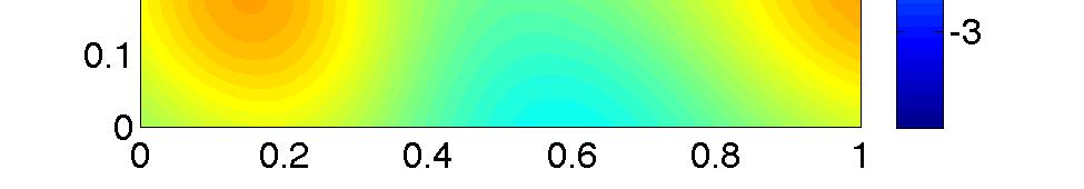
83 (a) True field at t = 1 (b) True field at t = 5 (c) Predicted field at t = 1 (d) Predicted field at t = 5 Figure 4.7: Simulation results at t = 1 and t = 5 obtained by the centralized sampling scheme for case 2. 71

84 (e) Prediction error variance at t = 1 (f) Prediction error variance at t = 5 Figure 4.7: Simulation results at t = 1 and t = 5 obtained by the centralized sampling scheme for case 2 (cont d). (a) Prediction error variance at t = 1 (b) Prediction error variance at t = 5 Figure 4.8: Simulation results obtained by the centralized sampling scheme for case 3. The trajectories of agents are shown in solid lines. 72

85 0.85 Cost function Number of iterations Figure 4.9: Cost function J d ( q) from t = 1 to t = 2 with a communication range R = Prediction error variance Prediction error variance t (a) R = t (b) R = 0.4 Figure 4.10: Average of prediction error variances over all target points and agents achieved by the distributed sampling scheme with a communication range (a) R = 0.3, and (b) R = 0.4. The average of prediction error variances over all target points and agents are shown in blue circles. The average of prediction error variance over local target points and agents are shown in red squares. The error-bars indicate the standard deviation among agents. 73

86 (a) R = 0.3, t = 1 (b) R = 0.3, t = 2 (c) R = 0.3, t = 5 (d) R = 0.3, t = 20 Figure 4.11: Simulation results obtained by the distributed sampling scheme with different communication ranges. The edges of the graph are shown in solid lines. 74

87 (e) R = 0.4, t = 1 (f) R = 0.4, t = 2 (g) R = 0.4, t = 5 (h) R = 0.4, t = 20 Figure 4.11: Simulation results obtained by the distributed sampling scheme with different communication ranges (cont d). The edges of the graph are shown in solid lines. 75

88 Chapter 5 Fully Bayesian Approach Recently, there has been an increasing exploitation of mobile sensor networks in environmental monitoring [10, 13, 35, 37]. Gaussian process regression (or kriging in geostatistics) has been widely used to draw statistical inference from geostatistical and environmental data [15,51]. For example, near-optimal static sensor placements with a mutual information criterion in Gaussian processes were proposed in [32]. A distributed kriged Kalman filter for spatial estimation based on mobile sensor networks was developed in [13]. Multi-agent systems that are versatile for various tasks by exploiting predictive posterior statistics of Gaussian processes were developed in [8, 9]. The significant computational complexity in Gaussian process regression due to the growing number of observations (and hence the size of covariance matrix) has been tackled in different ways. In [67], the authors analyzed the conditions under which near-optimal prediction can be achieved using only truncated observations. This motivates the usage of sparse Gaussian process proposed in [45]. However, they both assumed the covariance function is known a priori, which is unrealistic in practice. On the other hand, unknown parameters in 76

89 the covariance function can be estimated by the maximum likelihood (ML) estimator. Such ML estimates may be regarded as the true parameters and then used in the prediction [65]. However, the point estimate itself needs to be identified using sufficient amount of measurements. Instead, a maximum a posterior (MAP) estimate can use the prior to provide the point estimate with a small number of measurements. However, it fails to incorporate the uncertainty in the estimate into the prediction. The advantage of a fully Bayesian approach, which will be adopted in this work, is that the uncertainty in the model parameters are incorporated in the prediction [5]. In [22], Gaudard et al. presented a Bayesian method that uses importance sampling for analyzing spatial data sampled from a Gaussian random field whose covariance function was unknown. However, the assumptions made in [22], such as noiseless observations and time-invariance of the field, limit the applicability of the approach on mobile sensors in practice. The computational complexity of a fully Bayesian prediction algorithm has been the main hurdle for applications in resource-constrained robots. In [25], an iterative prediction algorithm without resorting to Markov Chain Monte Carlo (MCMC) methods has been developed based on analytical closed-form solutions from results in [22], by assuming that the covariance function of the spatio-temporal Gaussian random field is known up to a constant. Our work builds on such Bayesian approaches used in [22,25] and explores new ways to synthesize practical algorithms for mobile sensor networks under more relaxed conditions. In Section Section 5.1, we provide fully Bayesian approaches for spatio-temporal Gaussian process regression under more practical conditions such as measurement noise and the unknown covariance function. In Section 5.2, using discrete prior probabilities and compactly supported kernels, we provide a way to design sequential Bayesian prediction algorithms in 77

90 which the exact predictive distributions can be computed in constant time as the number of observations increases. In particular, a centralized sequential Bayesian prediction algorithm is developed in Section 5.2.1, and its distributed implementation among sensor groups is provided for a special case in Section An adaptive sampling strategy for mobile sensors, utilizing the maximum a posteriori (MAP) estimation of the parameters, is proposed to minimize the prediction error variances in Section In Section 5.3, the proposed sequential Bayesian prediction algorithms and the adaptive sampling strategy are tested under practical conditions for spatio-temporal Gaussian processes. 5.1 Fully Bayesian Prediction Approach In this chapter, we consider a spatio-temporal Gaussian process denoted by z(x) GP ( ) µ(x), σf 2 C(x, x ; θ), where z(x) R and x := (s T, t) T Q Z >0 contains the sampling location s Q R D and the sampling time t Z >0. The mean function is assumed to be µ(x) = f(x) T β, where f(x) := (f 1 (x),, f p (x)) T R p is a known regression function, and β R p is an unknown vector of regression coefficients. The correlation between z(x) and z(x ) is taken as ( s C(x, x s ) ( t t ) ; θ) = C s C t, (5.1) σ s σ t 78

91 which is governed by spatial and temporal distance functions C s ( ) and C t ( ). We assume that C s ( ) and C t ( ) are decreasing kernel functions over space and time, respectively, so that the correlation between two inputs decreases as the distance between spatial locations (respectively, time indices) increases. The decreasing rate depends on the spatial bandwidth σ s (respectively, the time bandwidth σ t ) for given fixed time indices (respectively, spatial locations). The signal variance σ 2 f gives the overall vertical scale relative to the mean of the Gaussian process in the output space. We define θ := (σ s, σ t ) T R 2 for notational simplicity. Given the collection of noise corrupted observations from mobile sensing agents up to time t, we want to predict z(s, t ) at a prespecified location s S Q and current (or future) time t. To do this, suppose we have a collection of n observations D = { } (x (i), y (i) ) i = 1,..., n from N mobile sensing agents up to time t. Here x (i) denotes the i-th input vector of dimension D + 1 (i.e., the sampling position and time of the i-th observation) and y (i) denotes the i-th noise corrupted measurement. If all observations are considered, we have n = Nt. Notice that the number of observations n grows with the time t. For notational simplicity, let y := (y (1),, y (n) ) T R n denote the collection of noise corrupted observations. Based on the spatio-temporal Gaussian process, the distribution of the observations given the parameters β, σf 2, and θ is Gaussian, i.e., y β, σ 2 f, θ N (F β, σ2 f C) 79

92 with F and C defined as ( F := f(x (1) ),, f(x )) (n) T R n p, [ C := Corr(y, y θ) = C(x (i), x (j) ; θ) + 1 ] γ δ ij R n n, (5.2) where δ ij is the Kronecker delta which equals to one when i = j, and zero, otherwise Prior selection To infer the unknown parameters β, σf 2, and θ in a Bayesian framework, the collection of them is considered to be a random vector with a prior distribution reflecting the a priori belief of uncertainty for them. In this chapter, we use the prior distribution given by π(β, σ 2 f, θ) = π(β σ2 f )π(σ2 f )π(θ), (5.3) where β σ 2 f N (β 0, σ 2 f T ). The prior for π(σf 2 ) is taken to be the inverse gamma distribution, chosen to guarantee positiveness of σ 2 f and a closed-form expression for the posterior distribution of σ2 f for computational ease of the proposed algorithms. To cope with the case where no prior knowledge on β is available, which is often the case in practice, we propose to use a noninformative prior. In particular, we take β 0 = 0, T = αi, and subsequently, let α. Any proper prior π(θ) that correctly reflects the priori knowledge of θ can be used. 80

93 5.1.2 MCMC-based approach According to the Bayes rule, the posterior distribution of β, σf 2, and θ is given by π(β, σf 2, θ y) = π(y β, σf 2, θ)π(β, σ2 f, θ) π(y β, σ 2 f, θ)π(β, σf 2,. (5.4) θ)dβdσ2 f dθ When a proper prior is used, the posterior distribution can be written as π(β, σ 2 f, θ y) π(y β, σ2 f, θ)π(β, σ2 f, θ). The inference on β, σf 2, and θ can be carried out by sampling from the posterior distribution in (5.4) via the Gibbs sampler. Table 5.1 gives the steps based on the following proposition. Table 5.1: Gibbs sampler. Input: initial samples β (1), σf 2 (1), and θ (1) { Output: samples β (i), σf 2 (i) } m, θ (i) from joint distribution π(β, i=1 σ2 f, θ y) 1: initialize β (1), σf 2 (1), θ (1) 2: for i = 1 to m do 3: sample β (i+1) from π(β σf 2 (i), θ (i), y) 4: sample σ 2 f (i+1) from π(σ 2 f β (i+1), θ (i), y) 5: sample θ (i+1) from π(θ β (i+1), σ 2 f (i+1), y) 6: end for Proposition For a prior distribution given in (5.3) with the noninformative prior on β, the conditional posteriors are given by 81

94 ( ) 1. β σf 2, θ, y N ˆβ, σ 2 f Σ ˆβ, where Σ ˆβ = (F T C 1 F ) 1, ˆβ = Σ ˆβ(F T C 1 y), 2. σ 2 f β, θ, y IG ( ā, b ), where ā = a + n + p, 2 1 b = b + 2 (y F β)t C 1 (y F β), 3. and π(θ β, σ 2 f, y) det(c) 1/2 exp ( (y F β)t C 1 (y F β) 2σ 2 f ) π(θ). Proof. Since the noninformative prior is chosen, the posterior distribution shall be computed with T = αi and then let α. i) For given σf 2, θ, and y, we have π(β σf 2 π(y β, σf 2, θ, y) = lim, θ)π(β σ2 f ) α π(y β, σ 2 f, θ)π(β σf 2)dβ. 82

95 Let num 1 = π(y β, σf 2, θ)π(β σ2 f ) { = exp 1 2σ f 2 (y F β) T C 1 (y F β) (2πσf 2)n/2 det(c) 1/2 { } } { } exp 1 2σ f 2 β T T 1 β (2πσf 2)p/2 det(t ) 1/2 exp 1 2σ 2 RSS { } f = (2πσf 2)(n+p)/2 det(c) 1/2 exp 1 det(t ) 1/2 2σf 2 (β ˆβ) T (F T C 1 F + T 1 )(β ˆβ), and den 1 = = { } exp 1 2σ f 2 RSS (2πσf 2)(n+p)/2 det(c) 1/2 det(t ) 1/2 { } { } exp 1 2σf 2 (β ˆβ) T (F T C 1 F + T 1 )(β ˆβ) dβ exp 1 2σ f 2 RSS (2πσf 2)(n+p)/2 det(c) 1/2 det(t ) 1/2 (2πσ2 f )p/2 det(f T C 1 F + T 1 ) 1/2 where RSS = y T ( C 1 C 1 F (F T C 1 F + T 1 ) 1 F T C 1) y = y T (C + F T F T ) 1 y. 83

96 Then we have π(β σf 2 num, θ, y) = lim 1 α den 1 { = lim α { = exp exp 1 2σ f 2 (β ˆβ) T (F T C 1 F + T 1 )(β ˆβ) (2πσf 2)p/2 det(f T C 1 F + T 1 ) 1/2 } 1 2σ f 2 (β ˆβ) T Σ 1 (β ˆβ) ˆβ (2πσf 2)p/2 det(σ ˆβ) 1/2. } Therefore, we have β σ 2 f, θ, y N ( ˆβ, σ 2 f Σ ˆβ). ii) For given β, θ, and y, we have π(σf 2 π(y β, σf 2 β, θ, y) = lim, θ)π(σ2 f β) α π(y β, σ 2 f, θ)π(σf 2 β)dσ2 f π(y β, σf 2 = lim, θ)π(β σ2 f )π(σ2 f ) α π(y β, σ 2 f, θ)π(β σf 2. )π(σ2 f )dσ2 f Let num 2 = π(y β, σf 2, θ)π(β σ2 f )π(σ2 f ) { = = exp 1 2σ f 2 (y F β) T C 1 (y F β) (2πσf 2)n/2 det(c) 1/2 b a 1 Γ(a)(2π)ā+1 det(c) 1/2 det(t ) 1/2 (σf 2 exp )ā+1 84 } { } exp 1 2σ f 2 β T T 1 β (2πσf 2)p/2 det(t ) 1/2 b a exp { b σ 2 f Γ(a)(σf 2 { )a+1 b β T T 1 } β σf 2, }

97 and den 2 = = b a Γ(a)(2π)ā+1 det(c) 1/2 det(t ) 1/2 b a Γ(a)(2π)ā+1 det(c) 1/2 det(t ) 1/2 Γ(ā) b ā. { 1 b + 1 (σf 2 exp 2 β T T 1 } β )ā+1 σf 2 dσf 2 Then we have π(σf 2 num β, θ, y) = lim 2 α den 2 = lim α = { bā b + 1 Γ(ā)(σf 2 exp 2 β T T 1 } β )ā+1 2σf 2 { bā Γ(ā)(σf 2 exp b } )ā+1 2σf 2. Therefore, we have σ 2 f β, θ, y IG ( ā, b ). iii) For given β, σf 2, and y, we have π(θ β, σf 2 π(y β, σf 2, y) = lim, θ)π(θ) α π(y β, σ 2 f, θ)π(θ)dθ ( det(c) 1/2 exp (y F β)t C 1 (y F β) 2σ 2 f ) π(θ). The posterior predictive distribution of z := z(s, t ) at location s and time t can be obtained by π(z y) = π(z y, β, σf 2, θ)π(β, σ2 f, θ y)dβdσ2 f dθ, (5.5) where in (5.5), the conditional distribution π(z β, σf 2, θ, y), is integrated with respect to the posterior of β, σ 2 f, and θ given observations y. The conditional distribution of z is Gaussian, 85

98 i.e., z β, σ 2 f, θ, y N (µ z β,σ 2 f,θ,y, σ2 z β,σ 2 f,θ,y), with µ z β,σ 2 f,θ,y = E(z β, σ 2 f, θ, y) = f(x ) T β + k T C 1 (y F β), σ 2 z β,σ 2 f,θ,y = Var(z β, σ 2 f, θ, y) = σ2 f (1 kt C 1 k), where k := Corr(y, z θ) = [K(x (i), x ; θ)] R n. To obtain numerical values of π(z y), we { draw m samples β (i), σf 2 (i) } m, θ (i) from the posterior distribution π(β, i=1 σ2 f, θ y) using the Gibbs sampler presented in Table 5.1, and then obtain the predictive distribution in (5.5) by π(z y) 1 m π(z y, β (i), σ 2 (i) m f, θ (i) ). i=1 It follows that the predictive mean and variance can be obtained numerically by µ z y = E(z y) 1 m µ m z i=1 β (i),σ f 2 (i),,θ (i),y ( σz y 2 = Var(z y) 1 m σ 2 m i=1 z β (i),σ f 2 (i) + 1 m 2 µ,θ (i),y m z i=1 β (i),σ f 2 (i) µ,θ (i) z,y y). Remark The Gibbs sampler presented in Table 5.1 may take long time to converge, which implies that the number of samples required could be quite large depending on the initial values. This convergence rate can be monitored from a trace plot (a plot of sampled values v.s. iterations for each variable in the chain). Moreover, since C is a complicated function of σ s and σ t, sampling from π(θ β, σf 2, y) in Proposition is difficult. An inverse cumulative distribution function (CDF) method [19] needs to be used to generate samples, which requires 86

99 griding on a continuous parameter space. Therefore, high computational power is needed to implement the MCMC-based approach. In the next subsection, we present an alternative Bayesian approach which only requires drawing samples from the prior distribution π(θ) using a similar approach to one used in [22] Importance sampling approach The posterior predictive distribution of z := z(s, t ) can be written as π(z y) = π(z θ, y)π(θ y)dθ, (5.6) where π(θ y) = π(y θ)π(θ) π(y θ)π(θ)dθ, is the posterior distribution of θ, by integrating out analytically the parameters β and σ 2 f. We have the following proposition. Proposition For a prior distribution given in (5.3) with the noninformative prior on β, we have 1. π(θ y) w(θ y)π(θ) with log w(θ y) = 1 2 log det(c) 1 2 log det(f T C 1 F ) ã log b, (5.7) 87

100 where ã = a + n 2, b = b yt C 1 y 1 2 (F T C 1 y) T (F T C 1 F ) 1 (F T C 1 y). 2. π(z θ, y) is a shifted student s t-distribution with location parameter µ, scale parameter λ, and ν degrees of freedom, i.e., π(z θ, y) = ( ) Γ ν+1 ( 2 λ Γ ( ν ) 2 πν )1 2 (1 + λ(z µ) 2 ν ) ν+1 2, (5.8) where ν = 2ã, and µ = k T C 1 y + (f(x ) F T C 1 k) T (F T C 1 F ) 1 (F T C 1 y), λ = b ( (1 k T C 1 k) + (f(x ) F T C 1 k) T (F T C 1 F ) 1 (f(x ) F T C 1 k) ). ã Proof. i) For given θ, we have π(y θ) = π(y β, σf 2, θ)π(β, σ2 f )dβdσ2 f = π(y β, σf 2, θ)π(β σ2 f )π(σ2 f )dβdσ2 f { } b a exp b+rss 2 σ f 2 = Γ(a)(2π) n/2 det(c) 1/2 det(t ) 1/2 det(f T C 1 F + T 1 ) 1/2 (σf 2 dσ 2 )n/2+a+1 f = Γ( n+2a 2 )b a ( Γ(a)(2π) n/2 det(c) 1/2 det(t ) 1/2 det(f T C 1 F + T 1 ) 1/2 b + RSS ) n+2a

101 where RSS = y T ( C 1 C 1 F (F T C 1 F + T 1 ) 1 F T C 1) y. As α, we have π(y θ)π(θ) π(θ y) = lim α π(y θ)π(θ)dθ det(c) 1/2 det(f T C 1 F ) (b 1/2 + 1 ) n+2a 2 yt 2 Σy, where Σ = C 1 C 1 F (F T C 1 F ) 1 F T C 1. ii) For given θ and y, we have π(z θ, y) = = π(z y, β, σ 2 f, θ)π(β, σ2 f θ, y)dβdσ2 f π(z y, β, σ 2 f, θ)π(β σ2 f, θ, y)π(σ2 f θ, y)dβdσ2 f, where ) z y, β, σf (f(x 2, θ N ) T β + k T C 1 (y F β), σf 2 (1 kt C 1 k), β σf 2, θ, y N ( ˆβ, σf 2 Σ ( ˆβ), σf 2 θ, y IG a + n 2, b + RSS ). 2 Then, it can be shown that π(z θ, y) = ( ) Γ ν+1 ( 2 λ Γ ( ν ) 2 πν )1 2 (1 + λ(z µ) 2 ν ) ν+1 2, 89

102 when α. The results in Proposition are different from those obtained in [22] by using a noninformative prior on β. For a special case where β and σ 2 f are known a priori, we have the following corollary which will be exploited to derive a distributed implementation among sensor groups in Section Corollary In the case where β and σ 2 f are known a priori, (5.7) and (5.8) can be simplified as log w(θ y) = 1 2 log det(c) 1 2 (y F β)t C 1 (y F β), ( ) z θ, y N f(x ) T β + k T C 1 (y F β), σf 2 (1 kt C 1 k). If we draw m samples {θ (i)} m from the prior distribution π(θ), the posterior predictive i=1 distribution in (5.6) can then be approximated by π(z y) w(θ (i) y)π(z θ (i), y) w(θ (i). y) It follows that the predictive mean and variance can be obtained by µ z y = E(z y) σ 2 z y = Var(z y) w(θ (i) y)µ z θ (i),y w(θ (i), y) w(θ (i) y)σ 2 z θ (i),y w(θ (i) y) + ( ) 2 w(θ (i) y) µ z θ (i),y µ z y w(θ (i), y) 90

103 where the mean and variance of the student s t-distribution π(z θ, y) are given by µ z θ,y = E(z θ, y) = µ, σ 2 z θ,y = Var(z θ, y) = ã ã 1 λ Discrete prior distribution To further reduce the computational demands from the Monte Carlo approach, we assign discrete uniform probability distributions to σ s and σ t as priors instead of continuous probability distributions. Assume that we know the range of parameters in θ, i.e., σ s [σ s, σ s ] and σ t [σ t, σ t ], where σ and σ denote the known lower-bound and upper-bound of the random variable σ, respectively. We constrain the possible choices of θ on a finite set of grid points denoted by Θ. Hence, π(θ) is now a probability mass function (i.e., θ Θ π(θ) = 1) as opposed to a probability density. The integration in (5.6) is reduced to the following summation π(z y) = θ Θ π(z θ, y)π(θ y), (5.9) where the posterior distribution of θ is evaluated on the grid points in Θ by π(θ y) = w(θ y)π(θ) (5.10) θ Θ w(θ y)π(θ). In order to obtain the posterior predictive distribution in (5.9), the computation of π(z θ, y) and w(θ y) for all θ Θ using the results from Proposition (or Corollary for a 91

104 special case) are necessary. Note that these quantities are available in closed-form which reduces the computational burden significantly. 5.2 Sequential Bayesian Prediction Although the aforementioned efforts in Sections and reduce the computational cost significantly, the number of observations (that mobile sensing agents collect) n increases with the time t. For each θ Θ, an n n positive definite matrix C needs to be inverted which requires time O(n 3 ) using standard methods. This motivates us to design scalable sequential Bayesian prediction algorithms by using subsets of observations Scalable Bayesian prediction algorithm The computation of π(z y 1:t ) soon becomes infeasible as t increases. To overcome this drawback while maintaining the Bayesian framework, we propose to use subsets of all observations y 1:t R Nt. However, instead of using truncated local observations only as in [67], Bayesian inference will be drawn based on two sets of observations: First, a set of local observations near target points ỹ which will improve the quality of the prediction, and second, a cumulative set of observations ȳ which will minimize the uncertainty in the estimated parameters. Taken together, they improve the quality of prediction as the number of observations increases. We formulate this idea in detail in the following paragraph. For notational simplicity, we define y R Nt as a subset of all observations y 1:t which will be used for Bayesian 92

105 prediction. We partition y into two subsets, namely ȳ and ỹ. Let F and F be the counterparts of F defined in (5.2) for ȳ and ỹ, respectively. The following lemma provides the conditions under which any required function of y in Proposition can be decoupled. Lemma For a given θ Θ, let C = Corr(y, y θ), C = Corr(ȳ, ȳ θ), C = Corr(ỹ, ỹ θ), k = Corr(y, z θ), k = Corr(ȳ, z θ), and k = Corr(ỹ, z θ). If the following conditions are satisfied C1: Corr(ỹ, ȳ θ) = 0, i.e., ỹ and ȳ are uncorrelated, and C2: Corr(ȳ, z θ) = 0, i.e., ȳ and z are uncorrelated, then we have the following results: F T C 1 F = F T C 1 F + F T C 1 F R p p, F T C 1 y = F T C 1ȳ + F T C 1ỹ R p, y T C 1 y = ȳ T C 1ȳ + ỹ T C 1ỹ R, log det C = log det C + log det C R, F T C 1 k = F T C 1 k R p, k T C 1 k = k T C 1 k R. Proof. The results follow by noting the correlation matrix C can be decoupled such that C = diag( C, C) and k = 0. Remark In order to compute the posterior predictive distribution π(z y) (or the predictive mean and variance) in (5.9), π(z θ, y) and π(θ y) for all θ Θ need to be calculated. Notice that the posterior distribution of θ can be obtained by computing w(θ y) in 93

106 (5.7). Suppose F T C 1 F R p p, F T C 1ȳ R p, ȳ T C 1ȳ R, and log det C R are known for all θ Θ. If F T C 1 F R p p, F T C 1ỹ R p, ỹ T C 1ỹ R, and log det C R for all θ Θ have fixed computation times, then (5.7) and (5.8) can be computed in constant time due to decoupling results of Lemma The following theorem provides a way to design scalable sequential Bayesian prediction algorithms. Theorem Consider the discrete prior probability π(θ) and the compactly supported kernel function φ t ( ). If we select η σ t Z >0, Z >0 and define c t := max ( ) t, 0 R, + η ξ j := y (j 1)( +η)+1:(j 1)( +η)+ R N, ȳ := (ξ T 1,, ξt c t ) T R Nc t, (5.11) ỹ := y t +1:t R N, where is the floor function defined by x := max {m Z m x}, then the posterior predictive distribution in (5.9) can be computed in constant time (i.e., does not grow with the time t). Proof. By construction, conditions C1-2 in Lemma are satisfied. Hence, it follows from Remark that the posterior predictive distribution can be computed in constant time. Remark In Theorem 5.2.3, η σ t guarantees the time distance between ξ j and ξ j+1 is large enough such that the conditions in Lemma are satisfied. Notice that is a tuning parameter for users to control the trade-off between the prediction quality and 94

107 the computation efficiency. A large value for yields a small predictive variance but long computation time, and vice versa. An illustrative example with three agents sampling the spatio-temporal Gaussian process in 1-D space is shown in Fig σ t (s,t ) space time 13 t = 15 Figure 5.1: Example with three agents sampling the spatio-temporal Gaussian process in 1-D space and performing Bayesian inference. In this example, σ t = 2.5, η = 2, = 3, t = 15, c t = 2, ȳ = (y T 1:3, yt 6:8 )T and ỹ = y 13:15. Based on Theorem 5.2.3, we provide the centralized sequential Bayesian prediction algorithm as shown in Table Distributed implementation for a special case In this subsection, we will show a distributed way (among agent groups) to implement the proposed algorithm for a special case in which β and σ 2 f are assumed to be known a priori. The assumption for this special case is the exact opposite of the one made in [25] where β and σ 2 f are unknown and θ is known a priori. To develop a distributed scheme among agent groups for data fusion in Bayesian statistics, we exploit the compactly supported kernel for space. Let C s (h) in (5.1) also be a compactly supported kernel function as C t (h) so that the correlation vanishes when the spatial distance between two inputs is larger than σ s, i.e., C s (h) = 0, h > 1. 95

108 Consider a case in which M groups of spatially distributed agents sample a spatiotemporal Gaussian process over a large region Q. Each group is in charge of its sub-region of Q. The identity of each group is indexed by V := {1,, M}. Each agent in group i is indexed by I [i] := {1,, N}. The leader of group i is referred to as leader i, which implements the centralized scheme to make prediction on its sub-region using local observations and the globally updated posterior distribution of θ. Therefore, the posterior distribution of θ shall be updated correctly using all observations from all groups (or agents) in a distributed fashion. Let G(t) := (V, E(t)) be an undirected communication graph such that an edge (i, j) E(t) if and only if leader i can communicate with leader j at time t. We define the neighborhood of leader i at time t by N i (t) := {j V (i, j) E(t), j i}. Let a [i] denote the quantity as a in the centralized scheme for group i. We then have the following theorem. Theorem Assume that ȳ [i] and ỹ [i] for leader i are selected accordingly to Theorem in time-wise. Let ỹ defined by ỹ := ((ỹ [1] ) T,, (ỹ [M] ) T ) T. If the following condition is satisfied C3: q [i] l (t) q[j] ν (t ) σ s, i j, l I [i], ν I [j], in the spatial domain, then the weights w(θ y), based on all observations from all agents, can be obtained from M log w(θ y) = log w(θ ȳ) + log w(θ ỹ [i] ). (5.12) i=1 Proof. The result follows by noting Corr(ỹ [i], ỹ [j] θ) = 0, i j, when the condition C3 is satisfied. An exemplary configuration of agents which satisfies C3 is shown in Fig

109 σ s σ s σ s Figure 5.2: Example with three group of agents sampling the spatio-temporal Gaussian process in 2-D space and performing Bayesian prediction. The symbol o denotes the position of a leader for a group and the symbol x denotes the position of an agent. Distance between any two sub-regions is enforced to be greater than σ s which enables the distributed Bayesian prediction. Suppose that the communication graph G(t) is connected for all time t. Then the average 1 M Mi=1 log w(θ ỹ [i] ) can be achieved asymptotically via discrete-time average-consensus algorithm [48]: log w(θ ỹ [i] ) log w(θ ỹ [i] ) + ɛ ( ) log w(θ ỹ [j] ) log w(θ ỹ [i] ), j N i with 0 < ɛ < 1/ (G) that depends on the maximum node degree of the network (G) = max i N i Adaptive sampling At time t, the goal of the navigation of agents is to improve the quality of prediction of the field Q at the next sampling time t + 1. Therefore, mobile agents should move to the most 97

110 informative sampling locations q(t+1) = (q 1 (t+1) T,, q N (t+1) T ) T at time t+1 in order to reduce the prediction error [32]. Suppose at time t + 1, agents move to a new set of positions q = ( q 1 T,, qt N )T. The mean squared prediction error is defined as J( q) = s S [ E (z(s, t + 1) ẑ(s, t + 1)) 2] ds, (5.13) where ẑ(s, t + 1) is obtained as in (5.9). Due to the fact that θ has a distribution, the evaluation of (5.13) becomes computationally prohibitive. To simplify the optimization, we propose to utilize a maximum a posteriori (MAP) estimate of θ at time t, denoted by ˆθ t, i.e., ˆθ t = arg max θ Θ π(θ y), where y is the subset of all observations used up to time t. The next sampling positions can be obtained by solving the following optimization problem q(t + 1) = arg min Var(z(s, t + 1) y, ˆθ t )ds. (5.14) q i Q s S This problem can be solved using standard constrained nonlinear optimization techniques (e.g., the conjugate gradient algorithm), possibly taking into account mobility constraints of mobile sensors. Remark The proposed control algorithm in (5.14) is truly adaptive in the sense that the new sampling positions are functions of all collected observations. On the other hand, if all parameters are known, the optimization in (5.14) can be performed offline without taking 98

111 any measurements. 5.3 Simulation In this section, we apply the proposed sequential Bayesian prediction algorithms to spatiotemporal Gaussian processes with a correlation function in (5.1). The Gaussian process was numerically generated through circulant embedding of the covariance matrix for the simulation study [20]. This technique allows us to numerically generate a large number of realizations of the Gaussian process MCMC-based approach on a 1-D scenario We consider a scenario in which N = 5 agents sample the spatio-temporal Gaussian process in 1-D space and the central station performs Bayesian prediction. The surveillance region Q is given by Q = [0, 10]. We consider the squared exponential function C s (h) = exp( 1 2 h2 ), for space correlation and a compactly supported correlation function [24] for time as (1 h) sin(2πh) 2πh + 1 cos(2πh) π 2πh C t (h) =, 0 h 1, 0, otherwise, (5.15) The signal-to-noise ratio γ is set to be 26dB which corresponds to σ w = The true values for the parameters used in simulating the Gaussian process are given by (β, σf 2, σ s, σ t ) = (0, 1, 2, 8). Notice that the mean function is assumed to be an unknown random variable, 99

112 i.e., the dimension of the regression coefficient β is 1. We assume that β σf 2 has the noninformative prior and σ 2 f IG(3, 20). The Gibbs sampler in Table 5.1 was used to generate samples from the posterior distribution of the parameters. A random sampling strategy was used in which agents make observations at random locations at each time t Z >0. The prediction was evaluated at each time step for 51 uniform grid points within Q. The histograms of the samples at time t = 1 and t = 10 are shown in Fig. 5.3-(a) and Fig. 5.3-(b), respectively. It is clear that the distributions of the parameters are centered around the true values with 100 observations at time t = 20. The prediction results at time t = 1 and t = 20 are shown in Fig. 5.4-(a) and Fig. 5.4-(b), respectively. However, with only 100 observations, the running time using the full Bayesian approach is about several minutes which will soon become intractable β σf β σf σ s σ t σ s σ t (a) (b) Figure 5.3: Posterior distribution of β, σ 2 f, σ s, and σ t at (a) t = 1, and (b) t = Centralized scheme on 1-D scenario We consider the same scenario in which N = 5 agents sample the spatio-temporal Gaussian process in 1-D space and the central station performs Bayesian prediction. The true values 100

113 (a) s s (b) Figure 5.4: Prediction at (a) t = 1, and (b) t = 20 using the MCMC-based approach. The true fields are plotted in blue solid lines. The predicted fields are plotted in red dash-dotted lines. The area between red dotted lines indicates the 95% confidence interval. for the parameters used in simulating the Gaussian process are given by (β, σ 2 f, σ s, σ t ) = (20, 10, 2, 8). Notice that the mean function is assumed to be an unknown random variable, i.e., the dimension of the regression coefficient β is 1. We assume that β σ 2 f has the noninformative prior and σf 2 IG(3, 20). We also assume the bounds of θ, viz. σ s [1.6, 2.4] and σ t [4, 12] are known. = 12 is used and η = 11 is selected satisfying the condition in Theorem We use a discrete uniform probability distribution for π(θ) as shown in Fig. 5.6-(a). The adaptive sampling strategy was used in which agents make observations at each time t Z >0. The prediction was evaluated at each time step for 51 uniform grid points within Q. Fig. 5.5 shows the comparison between predictions at time t = 1 using (a) the maximum likelihood (ML) based approach, and (b) the proposed fully Bayesian approach. The ML based approach first generates a point estimate of the hyperparameters and then uses them as true ones for computing the prediction and the prediction error variance. In this simulation, a poor point estimate on θ was achieved by maximizing the likelihood function. As a result, 101

114 the prediction and the associated prediction error variance are incorrect and are far from being accurate for a small number of observations. On the other hand, the fully Bayesian approach which incorporates the prior knowledge of θ and uncertainties in θ provides a more accurate prediction and an exact confidence interval. Using the proposed sequential Bayesian prediction algorithm along with the adaptive sampling strategy, the prior distribution was updated in a sequential manner. At time t = 100, the posterior distribution of θ is shown in Fig. 5.6-(b). With a larger number of observations, the support for the posterior distribution of θ becomes smaller and the peak gets closer to the true value. As shown in Fig. 5.7-(a), the quality of the prediction at time t = 100 is significantly improved. At time t = 300, the prior distribution was further updated which is shown in Fig. 5.6-(c). At this time, θ = (2, 8) T, which is the true value, has the highest probability. The prediction is also shown in Fig. 5.7-(b). This demonstrates the usefulness and correctness of our algorithm. The running time at each time step is fixed, which is around 12s using Matlab, R2008a (MathWorks) in a PC (2.4GHz Dual-Core Processor) Distributed scheme on 2-D scenario Finally, we consider a scenario in which there are 4 groups, each of which contain 10 agents sampling the spatio-temporal Gaussian process in 2-D space. The surveillance region Q is given by Q = [0, 10] [0, 10]. The parameter values used in simulating the Gaussian process are given by θ = (σ s, σ t ) T = (2, 8) T, β = 0, and σ 2 f = 1, last two values of which are assumed to be known a priori. To use the distributed scheme, we only consider compactly supported kernel functions for both space and time. In particular, we consider C s (h) = C t (h) as in 102

115 s (a) s (b) Figure 5.5: Prediction at t = 1 using (a) the maximum likelihood based approach, and (b) the proposed fully Bayesian approach. The true fields are plotted in blue solid lines. The predicted fields are plotted in red dash-dotted lines. The area between red dotted lines indicates the 95% confidence interval. (5.15). We also assume the fact that σ s [1.6, 2.4] and σ t [4, 12] are known a priori. = 12 is used and η = 11 is selected satisfying the condition in Theorem The region Q is divided into 4 square sub-regions with equal size areas as shown in Fig. 5.9-(a). Distance between any two sub-regions is enforced to be greater than σ s = 2.4, satisfying the condition in Theorem 5.2.5, which enables the distributed Bayesian prediction. The same uniform prior distribution for θ as in the centralized version (see Fig. 5.6-(a)) is used. The globally updated posterior distribution of θ at time t 100 is shown in Fig It has a peak near the true θ, which shows the correctness of the distributed algorithm. The predicted field compared with the true field at time t 100 is shown in Fig Due to the construction of sub-regions, the interface areas between any of two sub-regions are not predicted. Notice that the prediction is not as good as in the 1-D scenario due to the effect of curse of dimensionality when we move from 1-D to 2-D spaces. The prediction quality can be improved by using more number of sensors at the cost of computational time. The running time of the distributed algorithm in this scenario is about several minutes due to 103

116 σ t σ s σ t σ s (a) (b) σ t σ s (c) Figure 5.6: (a) Prior distribution θ, (b) posterior distribution of θ at time t = 100, (c) posterior distribution of θ at time t = 300. the complexity of the 2-D problem under the same computational environment as the one used for the 1-D scenario. However, thanks to our proposed sequential sampling schemes, the running time does not grow with the number of measurements. 104

117 s (a) s (b) Figure 5.7: Prediction at (a) t = 100, and (b) t = 300 using the centralized sequential Bayesian approach. The true fields are plotted in blue solid lines. The predicted fields are plotted in red dash-dotted lines. The area between red dotted lines indicates the 95% confidence interval σ t σ s Figure 5.8: Posterior distribution of θ at time t = 100 using the distributed algorithm. 105

118 Table 5.2: Centralized Bayesian prediction algorithm. Input: (1) prior distribution on σf 2, i.e., π(σ2 f ) = IG(a, b) (2) prior distribution on θ Θ, i.e., π(θ) (3) tuning variables and η (4) number of agents N (5) M(θ).A = 0 R p p, M(θ).B = 0 R, M(θ).C = 0 R p, M(θ).D = 0 R, M 0 (θ) = M(θ), θ Θ Output: (1) The predictive mean at location s S and time t = t, i.e., µ z y (2) The predictive variance at location s S and time t = t, i.e., σ 2 z y At time t, the central station does: 1: receive observations y t from agents, set ỹ = y t +1:t and n = N 2: compute F = (f( x (1) ),, f( x (n) )) T where x (i) is the input of the i-th element in ỹ 3: for each θ Θ do 4: compute C = Corr(ỹ, ỹ) R n n 5: compute the key values F T C 1 F = M(θ).A + F T C 1 F R p p, y T C 1 y = M(θ).B + ỹ T C 1ỹ R, F T C 1 y = M(θ).C + F T C 1ỹ R p, log det C = M(θ).D + log det C R 6: compute ã = a + n 2 and b = b y T C 1 y 1 2 (F T C 1 y) T (F T C 1 F ) 1 (F T C 1 y) 7: update weights via log w(θ y) = 1 2 log det C 1 2 log det(f T C 1 F ) ã log b 8: for each s S do 9: compute f(x ) R p, k = Corr(ỹ, z ) R n 10: compute predictive mean and variance for given θ µ z θ,y = k C 1 ỹ + (f(x ) F T C 1 k) T (F T C 1 F ) 1 (F T C 1 y), σ z θ,y 2 = b ã 1 ((1 k T C 1 k) + (f(x ) F T C 1 k) T (F T C 1 F ) 1 (f(x ) F ) T C 1 k) 11: end for 12: if mod(t, + η) = then 13: set M(θ) = M 0 (θ), then M 0 (θ).a = F T C 1 F, M 0 (θ).b = y T C 1 y, M 0 (θ).c = F T C 1 y, and M 0 (θ).d = log det C 14: end if 15: end for 16: compute the posterior distribution π(θ y) = w(θ y)π(θ) θ w(θ y)π(θ) 17: compute the predictive mean and variance µ z y = θ µ z θ,y π(θ y), σ z y 2 = θ σ2 z θ,y π(θ y) + ( 2 θ µ z θ,y z y) µ π(θ y). 106

119 (a) (b) Figure 5.9: Comparison of (a) the true field at t = 100 and (b) the predicted field at t = 100 using the distributed algorithm. 107

120 Chapter 6 Gaussian Process with Built-in GMRF Recently, there have been efforts to find a way to fit a computationally efficient Gaussian Markov random field (GMRF) on a discrete lattice to a Gaussian random field on a continuum space [17,27,56]. Such methods have been developed using a fitting with a weighted L 2 -type distance [56], using a conditional-mean least-squares fitting [17], and for dealing with large data by fast Kriging [27]. It has been demonstrated that GMRFs with small neighborhoods can approximate Gaussian fields surprisingly well [56]. This approximated GMRF and its regression are very attractive for the resource-constrained mobile sensor networks due to its computational efficiency and scalability [34] as compared to the standard Gaussian process and its regression, which is not scalable as the number of observations increases. Mobile sensing agents form an ad-hoc wireless communication network in which each agent usually operates under a short communication range, with limited memory and computational power. For resource-constrained mobile sensor networks, developing distributed 108

121 prediction algorithms for robotic sensors using only local information from local neighboring agents has been one of the most fundamental problems [4, 6, 10, 13, 25, 47]. In Section 6.1.1, a new class of Gaussian processes is proposed for resource-constrained mobile sensor networks. Such a Gaussian process builds on a GMRF [54] with respect to a proximity graph, e.g., the Delaunay graph of a set of vertices over a surveillance region. The formulas for predictive statistics are derived in Section We propose a sequential prediction algorithm which is scalable to deal with sequentially sampled observations in Section In Section 6.2, we develop a distributed and scalable statistical inference algorithm for a simple sampling scheme by applying the Jacobi over-relaxation and discretetime average consensus algorithms. Simulation and experimental study demonstrate the usefulness of the proposed model and algorithms in Section Spatial Prediction In this section, we first propose a new class of Gaussian random fields with built-in Gaussian Markov random fields (GMRF) [54]. Then we show how to compute the prediction at any point of interest based on Gaussian process regression, and provide a sequential field prediction algorithm for mobile sensor networks Spatial model based on GMRF Let γ := (γ(p 1 ),, γ(p m )) T N (0, Q 1 ) be a zero-mean GMRF [54] with respect to an undirected graph G = (V, E), where the location of vertex i is denoted by p i in the surveillance region Q. Such locations of vertices will be referred to as generating points. The inverse covariance matrix (precision matrix) Q 0 has the property (Q) ij 0 {i, j} E. 109

122 If the graph G has small cardinalities of the neighbor sets, its precision matrix Q becomes sparse with many zeros in its entries. This plays a key role in computation efficiency of a GMRF which can be greatly exploited by the resource-constrained mobile sensor network. The spatial field is modeled by a Gaussian process with a built-in GMRF defined as m z(s) = µ(s) + λ(s, p j )γ(p j ), (6.1) j=1 where λ(, ) is a weighting function. The new class of Gaussian processes is capable of representing a wide range of non-stationary Gaussian fields, by selecting 1. different number of generating points m, 2. different locations of generating points { p j j = 1,, m } over Q, 3. a different structure of the precision matrix Q, and 4. different weighting functions { λ(, p j ) j = 1,, m }. Remark The number of generating points could be determined by a model selection criterion such as the Akaike information criterion [1]. Similar to hyperparameter estimation in the standard Gaussian process regression, one can estimate all other parameters using maximum likelihood (ML) optimization [51, 65]. This is non-convex optimization and so the initial conditions need to be chosen carefully to avoid local minima. In our approach, we use basic structures for weighting functions and the precision matrix, however, we make them as functions of the locations of generating points. Different spatial resolutions can be obtained by a suitable choice of locations of generating points. As an example shown in Fig. 6.1, higher resolution can be obtained by higher density of generating points (see lower left corner). In 110

123 this way, we only need to determine the locations of generating points. This approach will be demonstrated with real-world data in Section (a) (b) Figure 6.1: (a) Generating points in blue dots and the associated Delaunay graph with edges in red dotted lines. The Voronoi partition is also shown in blue solid lines. (b) Gaussian random field with a built-in GMRF with respect to the Delaunay graph in (a) Gaussian process regression Suppose we have a collection of observations y := (y 1,, y n ) T whose entries are sampled at the corresponding points s 1,, s n. The noise corrupted measurement y i R is given by y i = z(s i ) + ɛ i, where ɛ i i.i.d. N (0, σ 2 w) is an independent and identically distributed (i.i.d.) Gaussian white noise. We then have the following results. Proposition Let Λ R n m be a matrix obtained by (Λ) ij = λ(s i, p j ) and let λ R m be a vector obtained by (λ) i = λ(s 0, p i ), where s 0 is a point of interest. Then the covariance 111

124 matrix of y and the covariance between y and z(s 0 ) are given by C := E[(y E y)(y E y) T ] = ΛQ 1 Λ T + σ 2 wi, k := E[(y E y)z(s 0 )] = ΛQ 1 λ, where Q R m m is the precision matrix of the GMRF γ R m. Proof. The (i, j)-th element of the covariance matrix C, i.e., the covariance between y i and y j, can be obtained by C ij = Cov(z(s i ), z(s j )) + σ 2 wδ ij = E(z(s i ) µ(s i ))(z(s j ) µ(s j )) + σwδ 2 ij ( ) ( ) = E λ(s i, p k )γ(p k ) λ(s j, p l )γ(p l ) + σwδ 2 ij k l = E k,l λ(s i, p k )γ(p k )γ(p l )λ(s j, p l ) + σwδ 2 ij = k,l λ(s i, p k ) E(γ(p k )γ(p l ))λ(s j, p l ) + σ 2 wδ ij = k,l λ(s i, p k )(Q 1 ) kl λ(s j, p l ) + σ 2 wδ ij. The i-th element of the covariance vector k, i.e., the covariance between y i and z(s 0 ), 112

125 can be obtained by k i = Cov(z(s i ), z(s 0 )) = E(z(s i ) µ(s i ))(z(s 0 ) µ(s 0 )) ( ) ( ) = E λ(s i, p k )γ(p k ) λ(s 0, p l )γ(p j ) k l = E λ(s i, p k )γ(p k )γ(p l )λ(s 0, p l ) k,l = k,l λ(s i, p k ) E(γ(p k )γ(p l ))λ(s 0, p l ) = k,l λ(s i, p k )(Q 1 ) kl λ(s 0, p l ), whose matrix form completes the proof. By Propositions 6.1.2, we can make prediction at the point of interest s 0 using Gaussian process regression [51]. This is summarized by the following theorem. Theorem For given y, the prediction of z 0 := z(s 0 ) at any location s 0 Q is given by the conditional distribution z 0 y N ( ) µ z0 y, σ2 z 0 y, where the predictive mean and variance are obtained by µ z0 y = µ(s 0) + λ T ˆQ 1ŷ, σ 2 z 0 y = λt ˆQ 1 λ, (6.2) 113

126 with ˆQ = Q + σ 2 w Λ T Λ R m m, ŷ = σ 2 w Λ T (y µ) R m. Proof. By using the Woodbury matrix identity (see Appendix A.2.1), the prediction mean can be obtained by µ z0 y = µ(s 0) + k T C 1 (y µ) = µ(s 0 ) + (ΛQ 1 λ) T (ΛQ 1 Λ T + σ 2 wi) 1 (y µ) = µ(s 0 ) + λ T Q 1 Λ T (ΛQ 1 Λ T + σ 2 wi) 1 (y µ) = µ(s 0 ) + λ T Q 1 Λ T (σ 2 w I σ 2 w Λ(Q + σ 2 w Λ T Λ) 1 Λ T σ 2 w )(y µ) = µ(s 0 ) + λ T (σ 2 w Q 1 σ 4 w Q 1 Λ T Λ(Q + σ 2 w Λ T Λ) 1 )Λ T (y µ) = µ(s 0 ) + λ T ΞΛ T (y µ), 114

127 where Ξ = σ 2 w Q 1 σ 4 w Q 1 Λ T Λ(Q + σ 2 w Λ T Λ) 1 = σ 2 w Q 1 (Q + σ 2 w Λ T Λ)(Q + σ 2 w Λ T Λ) 1 σ 4 w Q 1 Λ T Λ(Q + σ 2 w Λ T Λ) 1 = (σ 2 w I + σ 4 w Q 1 Λ T Λ)(Q + σ 2 w Λ T Λ) 1 σ 4 w Q 1 Λ T Λ(Q + σ 2 w Λ T Λ) 1 = σ 2 w (Q + σ 2 w Λ T Λ) 1. Similarly, the prediction error variance can be obtained by σ 2 z 0 y = λt Q 1 λ k T C 1 k = λ T Q 1 λ (ΛQ 1 λ) T (ΛQ 1 Λ T + σ 2 wi) 1 (ΛQ 1 λ) = λ T ( Q 1 Q 1 Λ T (ΛQ 1 Λ T + σ 2 wi) 1 ΛQ 1) λ = λ T (Q + σ 2 w Λ T Λ) 1 λ, where Cov(z(s 0 ), z(s 0 )) = λ T Q 1 λ is obtained similarly as in Proposition Remark When the generating points {p 1, p 2,, p m } are not known a priori, they can be estimated by maximizing the likelihood function. Given n observations y = (y 1, y 2,, y n ) T sampled at {s 1, s 2,, s n }, the log likelihood of y is given by log π(y) = 1 2 (y µ)t C 1 (y µ) 1 2 log det C n log 2π, 2 where C = ΛQ 1 Λ T + σ 2 wi is the covariance matrix of y. the maximum likelihood estimate 115

128 of the generating points can be obtained via solving the following optimization problem. ˆp ML = arg max log π(y). (6.3) p Remark Note that the number of generating points m is fixed and the number of observations n may grow in time, and so in general we consider m n. Theorem shows that only the inversion of an m m matrix ˆQ = Q+σ 2 w Λ T Λ is required in order to compute the predictive distribution of the field at any point. The computational complexity grows linearly with the number of observations, i.e., O(nm 2 ), compare to the standard Gaussian process regression which requires O(n 3 ). Moreover, it enables a scalable prediction algorithm for sequential measurements. In what follows, we present a sequential field prediction algorithm for sequential observations by exploiting the results of Theorem Sequential prediction algorithm Consider a sensor network consisting of N mobile sensing agents distributed in the surveillance region Q. The index of the robotic sensors is denoted by I := {1,, N}. The sensing agents sample the environmental field at time t Z >0 and send the observations to a central station which is in charge of the data fusion. At time t, agent i makes an observation y i (t) at location s i (t). Denote the collection of observations at time t by y t := (y 1 (t),, y N (t)) T. We have the following proposition. Proposition At time t Z >0, the predictive mean and variance at any point of 116

129 interest can be obtained via (6.2) with ˆQ t = ˆQ t 1 + σ 2 w Λ T t Λ t, ˆQ0 = Q ŷ t = ŷ t 1 + σ 2 w Λ T t (y t µ t ), ŷ 0 = 0, where (Λ t ) ij = λ(s i (t), s j (t)), and (µ t ) i = µ(s i (t)). Proof. The result can be obtained easily by noting that A T A = A T 1 A 1 + A T 2 A 2, where A = (A T 1, AT 2 )T. Based on Proposition 6.1.6, we present a sequential field prediction algorithm using mobile sensor networks in Table 6.1. Table 6.1: Sequential algorithm for field prediction. Input: a set of target points S Output: (1) prediction mean {ẑ(s 0 ) s 0 S} (2) prediction error variance { σ 2 (s 0 ) s 0 S } Assumption: (1) the central station knows p, Q, and λ(, ) (2) the central station initially has ˆQ Q, ŷ 0 At time t, agent i I in the network does: 1: take measurement y i from its current location s i 2: send the measurement (s i, y i ) to the central station At time t, the central station does: 1: obtain measurements {(s l, y l ) l I} from mobile sensors 2: compute Λ via (Λ) ij = λ(s i, p j ) 3: update ˆQ ˆQ + σw 2 Λ T Λ 4: update ŷ ŷ + σw 2 Λ T (y µ), where µ i = µ(s i ) 5: for s 0 S do 6: compute (λ) i via λ(s 0, p i ) 7: compute ẑ(s 0 ) = µ(s 0 ) + λ T ˆQ 1ŷ 8: compute σ 2 (s 0 ) = λ T ˆQ 1 λ 9: end for 117

130 6.2 Distributed Spatial Prediction In this section, we propose a distributed approach, in which robotic sensors exchange only local information between neighbors, to implement the field prediction effectively fusing all observations collected by all sensors correctly. This distributed approach can be implemented for a class of weighting functions λ(, ) in (6.1) that have compact supports. In particular, we consider the weighting function defined by λ(s, p j ) = λ( s pj /r), (6.4) where (1 h) cos(πh) + π 1 sin(πh), h 1, λ(h) := 0, otherwise. Notice that the weighting function λ(, ) in (6.4) has a compact support, i.e., λ(s, p j ) is non-zero if and only if the distance s pj is less than the support r R> Distributed computation We first briefly introduce distributed algorithms for solving linear systems and computing the averages. They will be used as major tools for distributed implementation of field prediction. Jacobi over-relaxation method: The Jacobi over-relaxation (JOR) [4] method provides an iterative solution of a linear system Ax = b, where A R n n is a nonsingular matrix and x, b R n. If agent i knows the row i (A) R n and b i, and a ij = (A) ij = 0 118

131 if agent i and agent j are not neighbors, then the recursion is given by x (k+1) i = (1 h)x (k) i + h b a i a ij x (k) j. (6.5) ii j N i This JOR algorithm converges to the solution of Ax = b from any initial condition if h < 2/n [13]. At the end of the algorithm, agent i knows the i-th element of x = A 1 b. Discrete-time average consensus: The Discrete-time average consensus (DAC) provides a way to compute the arithmetic mean of elements in the a vector c R n. Assume the graph is connected. If agent i knows the i-th element of c, the network can compute the arithmetic mean via the following recursion [47] x (k+1) i = x (k) i + ɛ a ij (x (k) j j N i x (k) i ), (6.6) with initial condition x(0) = c, where a ij = 1 if j N i and 0 otherwise, 0 < ɛ < 1/, and = max i ( j i a ij) is the maximum degree of the network. After the algorithm converges, all node in the network know the average of c, i.e., n i=1 c i /n Distributed prediction algorithm Consider a GMRF with respect to a proximity graph G = (V, E) that generates a Gaussian random field in (6.1). The index of the generating points is denoted by V := {1,, n}. The location of the i-th generating point is p i. The edges of the graph are considered to be E := { {i, j} } pi p j R, where R is a constant that ensures the graph is connected. Consider a mobile sensor network consisting of N mobile sensing agents distributed in the surveillance region Q. For simplicity, we assume that the number of agents is equal to 119

132 the number of generating points, i.e., N = m. The index of the robotic sensors is denoted by I := {1,, m}. The location of agent i is denoted by s i. The assumptions made for the resource-constrained mobile sensor networks are listed as follows. A.1 Agent i is in charge of sampling at point s i within a r-disk centered at p i, i.e., s i p i < r. A.2 r is the radius of the support of the weighting function in (6.4) and also satisfies that 0 < r < R 2. A.3 Agent i can only locally communicate with neighbors in N i := {j I {i, j} E} defined by the connected proximity graph G = (V, E). A.4 Agent i knows row i (Q), i.e., the i-th row of Q, where (Q) ij 0 if and only if j {i} N i. Remark As in A.1, it is reasonable to have at least one agent collect measurements that are correlated with a random variable from a single generating point. This sampling rule may be modified such that a single agent dynamically samples for multiple generating points or more number of agents samples for a generating point depending on available resources. Since there is at least one agent in charge of a generating point by A.1, it is natural to have A.3 and A.4 taking advantage of the proximity graph for the GMRF. Notice that each agent only knows local information of Q as described in A.4. An illustration of agent l sampling a measurement at point s l in the intersection of the supports of the weighting functions of p i and p j is shown in Fig From A.1 and A.2, since R > 2r, we have λ(s l, p i ) = 0 if l / N i. Thus the matrix ˆQ = Q + σ 2 w Λ T Λ R m m and the vector ŷ = σ 2 w Λ T (y µ) R m can be obtained in the 120

133 r p i s p j p k Figure 6.2: Example of computing (Λ T Λ) ij = λ(s l, p i )λ(s l, p j ). following form. ( ˆQ) ij = (Q) ij + σw 2 λ(s l, p i )λ(s l, p j ), } l {{i} N i } {{j} N j (ŷ) i = σw 2 λ(s l, p i )(y l µ l ). l {i} N i (6.7) Notice that ˆQ has the same sparsity as Q. From (6.7), A.3 and A.4, agent i can compute row i ( ˆQ) and (ŷ) i by using only local information from neighbors. Using row i ( ˆQ) and (λ) i, agent i can obtain the i-th element in the vector ˆQ 1 λ = (Q+σ 2 w Λ T Λ) 1 λ via JOR by using only local information. Finally, using (ŷ) i and (λ) i the prediction mean and variance can be obtained via the discrete-time average consensus algorithm. Notice that the sequential update of ˆQ and ŷ for sequential observations proposed in Section can be also applied to the distributed algorithm. The distributed algorithm for sequential field prediction under assumptions A.1-4 is summarized in Table 6.2. The number of robotic sensors and the sampling rule can be modified or optimized to maintain a better quality of the prediction and the corresponding distributed algorithm may 121

134 Table 6.2: Distributed algorithm for sequential field prediction. Input: (1) a set of target points S (2) the topology of sensor network G = (I, E) in which E := { {i, j} } pi p j R Output: { (1) prediction mean (2) prediction error variance } µ z0 y s 0 S { σ 2 z 0 y s 0 S } Assumption: (A1) agent i I is in charge of sampling at point s i within a r-disk centered at p i, i.e., s i p i < r (A2) the radius of the support of the weighting function satisfies 0 < r < R 2 (A3) agent i I can only locally communicate with neighbors N i := {j I {i, j} E} defined by the connected graph G = (V, E) (A4) agent i I initially has row i ( ˆQ) row i (Q), (ŷ) i 0 At time t, agent i I in the network does the following concurrently: 1: take measurement y i from its current location s i 2: update row i ( ˆQ) row i ( ˆQ) + row i (σ 2 w Λ T Λ) by exchanging information from neighbors N i 3: update (ŷ) i (ŷ) i + (σ 2 w Λ T (y µ)) i by exchanging information from neighbors N i 4: for s 0 S do 5: compute (λ) i = λ(s 0, p i ) 6: compute ( ˆQ 1 λ) i via JOR 7: compute µ z0 y = µ(s 0) + λ T ˆQ 1ŷ via DAC 8: compute σ 2 z 0 y = λt ˆQ 1 λ via DAC 9: end for be derived in a same way accordingly. 6.3 Simulation and Experiment In this section, we apply the proposed schemes to both simulation and experimental study. 122

135 6.3.1 Simulation We first apply our proposed prediction algorithms to a numerically generated Gaussian random field z( ) based on a GMRF with respect to a graph G = (V, E) defined in (6.1). The mean function µ( ) is assumed to be constant and µ = 5 is used in the simulation. We assume the generating points of the GMRF, indexed by V = {1,, n} where n = 30, are located at {p 1,, p n } in a 2-D unit area Q. The edges of the graph are assumed to be E := { {i, j} } p i p j R, where R = 0.4. The GMRF γ = (γ(p 1 ),, γ(p n )) T has a zero-mean and the precision matrix Q is given by (Q) ij = N (i) + c 0, if j = i, 1, if j N (i), 0, otherwise, where N (i) denotes the degree of node i, i.e., the number of connections it has to other nodes, c 0 = 0.1 is used to ensure Q is positive definite since a Hermitian diagonally dominant matrix with real non-negative diagonal entries is positive semi-definite [54]. We use compactly supported weighting functions defined in (6.4) for both centralized and distributed schemes with different support r. The sensor noise level is given by σ w = 0.5. Since the optimal sampling is beyond the scope of this chapter, in the simulation, we use a random sampling strategy in which robotic sensors sample at random locations at each time instance Centralized scheme We first consider a scenario in which N = 5 agents take samples in the surveillance region D at certain time instance t Z >0 and send the observations to a central station in which 123

136 the prediction of the field is made. The Gaussian random field z( ) is shown in Fig. 6.3-(a) with the n = 30 generating points of the built-in GMRF shown in black circles. The predicted field at times t = 1, t = 5, and t = 20 are shown in Figs. 6.3-(b), (c), and (d), respectively. The sampling locations are shown in black crosses. Clearly, the predicted field gets closer to the true field as the number of observations increases. The computational time for field prediction at each time instance remains fixed due to the nice structure of the proposed Gaussian field in (6.1) and its consequent results from Theorem Distributed scheme Next, we consider a scenario in which prediction is implemented in a distributed fashion (Table 6.2) under assumptions A.1-4 for the resource-constrained mobile sensor network in Section In particular, N = 30 robotic sensors are distributed according to the graph G = (V, E), which is connected. Agent i is in charge of the sampling with in a r-disk centered at p i, where the support r = 0.2 is used. Agent i has a fixed neighborhood, i.e., N (i) = {j {i, j} E}. In the simulation, h = 0.02 in (6.5) and ɛ = 0.02 in (6.6) are chosen to ensure the convergence of the JOR algorithm and the DAC algorithm. Fig. 6.4-(a) shows the underlying graph G = (V, E) for the GMRF with the generating points denoted by black circles and the edges in red lines. The sparsity of the precision matrix Q is shown in Fig. 6.4-(b). Notice that only 316 out of 900 elements in Q are nonzero which enables the efficient distributed computation. The true and the predicted fields at time t = 5 are shown in Figs. 6.5-(a) and (b), respectively. The normalized RMS error computed over about grid points at time t = 5 is 7.8%. The computational time at 124

137 (a) (b) (c) (d) Figure 6.3: Simulation results for the centralized scheme. (a) The true field, (b) the predicted field at time t = 1, (c) the predicted field at time t = 5, (d) the predicted field at time t = 20. The generating points are shown in black circles, and the sampling locations are shown in black crosses. each time instance remains fixed due to the nice structure of the proposed Gaussian field in (6.1) and its consequent results from Theorem

138 (a) (b) Figure 6.4: (a) Graph G = (V, E). (b) Sparsity structure of the precision matrix Q (a) (b) Figure 6.5: Simulation results for the distributed scheme. (a) The true field, (b) the predicted field at time t = 5. The generating points are shown in circles, and the sampling locations are shown in crosses Experiment In order to show the practical usefulness of the proposed approach, we apply the centralized scheme in Theorem on an experimentally obtained observations. We first measured 126