LECTURE NOTES ON THE Planetary Boundary Layer

Transcription

1 LECTURE NOTES ON THE Planetary Boundary Layer Chin-Hoh Moeng prepared for lectures given at the Department of Atmospheric Science, CSU in 1994 & 1998 and at the Department of Atmospheric and Oceanic Sciences, UCLA in INTRODUCTION 1.1 The nature of turbulence (see Appendix) 1.2 Averaging: statistics vs. instantaneous flow field 1.3 Governing equations Navier-Stokes equation Reynolds equation (or ensemble-mean equation) 1.4 Commonly-used terminology Energy-containing eddies and Kolmogorov microscale Reynolds number and Reynolds-number-independent regime Homogeneous and isotropic turbulence Quasi-steady state; large-eddy turnover time Inertial subrange and Kolmogorov theory 1.5 Research tools: field measurements, lab, LES, PBL modeling Understanding turbulent motions Modeling ensemble-mean statistics 2. THE SURFACE LAYER 2.1 Eddy structures 2.2 Monin-Obukhov similarity theory 1

2 3. THE CLEAR CONVECTIVE PBL 3.1 Thermal or plume structures 3.2 Scaling parameters and typical statistics profiles for the CBL 3.3 Scaling parameters and typical statistics profiles for weakly convective near-neutral PBL 3.4 Spectra 3.5 Scalar transport Countergradient transport Transport asymmetry Dispersion property 4. THE NEUTRAL AND STABLE PBLs 4.1 The neutral PBL 4.2 The weakly stable PBL 4.3 The very stable PBL 4.4 Physical phenomena in the stable PBL 5. BOUNDARY-LAYER CLOUDS 5.1 Stratocumulus clouds Physical processes Decoupling Diurnal cycle Cloud-top entrainment instability (CTEI) Vertical distributions of turbulence statistics 2

3 5.1.6 Climate-related issues 5.2 Shallow cumulus Interaction between cloud and subcloud layers Subcloud-layer spectra and statistics Climate impact 6. PBL MODELS (PARAMETERIZATIONS) 6.1 Higher-order closure model (or single-point closure) Higher-moment equations and closure problems The Mellor-Yamada model Realizability issue Applications to cloud-free PBLs Applications to stratocumulus-topped PBLs Examination of closure assumptions and constants 6.2 Richardson-number-dependent K model 6.3 K-profile model 6.4 The mixed-layer (bulk) modeling Model framework Entrainment closure based on the TKE budget of the whole PBL Entrainment closure based on the TKE budget in the entrainment zone Entrainment closure for the stratocumulus-topped PBL 6.5 Transilient turbulence theory/integral closure model 6.6 Mass flux model 6.7 Hybrid modeling approach 3

4 1 INTRODUCTION 1.1 The nature of turbulence No one describes the nature of turbulence better than Tennekes and Lumley. In their classic book (A First Course in Turbulence, 1972), Tennekes and J. L. Lumley list seven important characteristics of turbulent flows: irregularity, diffusivity, large Reynolds number, threedimensional vorticity fluctuations, dissipation, continuum, and turbulent flows are flows. An excerpt that describes these characteristics from their pages 1-4 is given in the Appendix for your reference. 1.2 Averaging: statistics vs. instantaneous flow field Because the details of the randomly-distributed turbulent field don t mean much, turbulence is often described by its averaged properties. Averaged properties are called statistics, including mean (expected) values (1st moments), fluxes and variances (2nd moments), skewness (3rd moment), probability density distribution, power spectrum, etc. To derive these statistics, we decompose a turbulent quantity to mean and fluctuating parts as u = u + u where u is defined by an averaging procedure (filtering procedure). Statistics, such as variance, are then computed as u u. Every time you look at a statistical measure, it is useful to know the type of averaging behind the measure. The most traditional description of turbulence uses ensemble averaging over a large samples of flow realizations such that all random turbulent motions can be removed by the average. Ensemble mean represents the expected outcome (or value) of the event. However, true ensemble average of geophysical turbulence is difficult to obtain because a turbulent event never repeats itself. In practice, we approximate ensemble averaging with spatial averaging (of, e.g., aircraft measurements) or time averaging (of, e.g., tower data). A time averaging of the turbulent plume of a smokestack downstream of a point source in a wind tunnel can be viewed from a long-time exposure camera, shown in Fig The top figure is the random instantaneous flow field of the event and the bottom is an time-averaged (or filtered) field. 4

5 Figure 1.1 (SOURCE: EPA Fluid Modeling Facility) If a turbulent flow field is horizontally homogeneous and quasi-steady, as we often assume for the PBL over uniform surface, then a horizontal averaging over a long distance or a large horizontal domain may represent an ensemble average. How time and spatial averages converge to ensemble average is a sampling problem. The flight length of an aircraft dataset or the time record of tower data has to be long enough so the statistics using a line (or time) averaging can approach ensemble-mean statistics. But the sample length cannot be too long to violate the horizontally homogeneous (or quasi-steady) assumption. As discussed in Lectures on the Planetary Boundary Layer by John Wyngaard in the book Mesoscale Meteorology Theories, Observations and Models, edited by Lilly and Gal-Chen, NATO ASI Series, the averaging time period (or length) is proportional to the integral scale and the intensity of the turbulent flow field. 5

6 1.3 Governing equations The before and after averaging of a turbulent flow field mentioned above can be described by its corresponding governing equations: Navier-Stokes equation and the Reynolds equation, as described below Navier-Stokes equation governing the whole turbulent motion The Navier-Stokes equation is the most fundamental dynamical equation of a viscous incompressible fluid. The flow field of a fluid at any time, t, and space, x i, is governed by u i t + u u i j = X i 1 p + ν 2 u i, (1) x j ρ x i where X i is the i-component of external forces, p pressure fluctuations, and ν the kinematic viscosity of the fluid. Along with the continuity eq., x 2 j u i x i = 0, (2) the set of equation is complete; there are four equations for four unknowns u, v, w and p. Notice the molecular term appears in the Navier-Stokes equation and the solution u i (x, y, z, t) includes all scales of motions, down to dissipation scales. When the non-linear interaction term (i.e., u j u i / x j ) is much larger than the molecular viscous term (i.e., ν 2 u i ), the solution of (1) is a fully developed turbulent motion. The x 2 j ratio of these two terms is called Reynolds number, which will be described in next section. The non-linear term includes vortex stretching and scrambling and energy cascading in 3D turbulence Reynolds equation (or ensemble-mean equation) Reynolds equation is the ensemble average of the Navier-Stokes equation. Reynolds equation is what we solve in GCMs or mesoscale models, not the Navier-Stokes equation. The solution of Reynolds equation does not explicitly contain turbulent motions because the chaotic turbulent component of the flow is filtered out, as you can see from the following derivation of the Reynolds equation. 6

7 To derive the Reynolds equation, we decompose a variable, s, into a Reynolds (or ensemble) mean component (denoted by overbar), s, and its fluctuation (or random turbulent) component (by prime), s, i.e., s = s + s. (3) The Reynolds averaging obeys the following rules: s = 0, ws = w s + w s, w + s = w + s, as = as, (4) where a is a constant, and w is another variable. With this averaging, the cross terms ws and w s are exactly zero. These rules imply that there is a spectral gap between the mean motion and the filtered out turbulent motions. By expanding Eq. (1) over a reference atmosphere state (denoted by the subscript 0) and decomposing it into the Reynolds mean and fluctuations, we have ( u i t + u i t )+(u j u i u i +u j +u u i j x j x j +u u i j x j ) = g i (θ+θ ) 1 p 1 p +ν 2 u i +ν 2 u i. x j T 0 ρ 0 x i ρ 0 x i The only external force we consider here is the buoyancy force, i.e., X i = g i /T 0 θ. Using the averaging rules (4) in (5) yields u i t + u u i j = + g i θ 1 p u iu j x j T 0 ρ 0 x i x j x 2 j x 2 j (5) + ν 2 u i, (6) x 2 j where the u iu j term is the so-called Reynolds stress term. For geophysical flows, the molecular term in (6) is several orders of magnitude smaller than the Reynolds stress term and can be neglected. Geophysical turbulence is often referred to as high Reynolds number flow. Thus, the Reynolds equation we solve in GCM or mesoscale models is u i t + u u i j = + g i θ 1 p u iu j, (7) x j T 0 ρ 0 x i x j where the Reynolds stress term represents the net effect of all filtered-out turbulent motions; none of the turbulent motion is explicitly included in the resolved field u i. The solution of (7) (i.e., u i ) is the ensemble mean of that of (1) (i.e., u i ). To solve (7) the Reynolds stress term needs to be parameterized, i.e., the stress term needs to be expressed in terms of the solvable variables. This is a closure problem, to close 7

8 the system of the governing equation. The simplest way to handle the closure problem is to assume that turbulent motions behave like molecular motions. This yields the constant eddy viscosity assumption where the stress term u iu j x j = K 2 u i, (8) x 2 j and then (7) would look just like (1, with X = g i T 0 θ) except that turbulent eddy viscosity K now replaces the molecular viscosity ν. But of course turbulence does not behave like molecular motions and that s why constant eddy viscosity cannot work. Some turbulence models close the (7) system by carrying yet more prognostic equations for the Reynolds stress, an approach referred to as higher-order closure modeling approach. We will learn about various types of PBL models in Section 6. For now, it is useful to know how the governing equations (or budgets) of higher-moment statistics (such as Reynolds stress or turbulent kinetic energy) look like. Equations for higher-moment statistics can be formally derived based on the eqs. of velocity (and of course temperature and moisture) fluctuations [see ref.: C. du. P. Donaldson, 1973: Construction of a Dynamic Model of the Production of Atmospheric Turbulence and the Dispersal of Atmospheric Pollutions, Workshop on Micrometeorology, published by the AMS], which are obtained by subtracting the mean, (6), from the total, (5), u i t + u u i j + u u i j + u u i j u j x j x j x j u i = + g i θ 1 p x j T 0 ρ 0 + ν 2 u i x i x 2 j. (9) For example, the equations for the Reynolds stress u iu j can be obtained by (a) multiplying (9) by u j, (b) multiplying (9) for u j by u i, (c) summing them up, and (d) applying Reynolds averaging. This yields a set of equations for u iu j. The ensemble-mean and fluctuating equations for scalars can be derived the same way. In deriving these equations, we further assume horizontal homogeneity, i.e., Φ/ x = Φ/ y = 0, where Φ is a statistical quantity. This assumption is referred to as the PBL assumption. Under this assumption, none of the horizontal fluxes shows up in the moment equations; there are only vertical derivatives of the vertical turbulent fluxes. But be cautious: This doesn t mean that the horizontal turbulence fluxes are zero; the horizontal fluxes can be as large as the vertical fluxes in the PBL. Because of the horizontal homogeneous assumption 8

9 (more in next section), horizontal convergence/divergence of the horizontal fluxes is assumed to be zero. Homework 1: A. Normalize the Navier-Stokes equation (assuming no external forcing) using a velocity scale U and a length scale L and show that the dimensionless equation contains only one dimensionless parameter. What is it? B. Derive the Poisson s equation for pressure from (1) and (2) and describe each term based on where it comes from. C. Derive the Reynolds-averaged turbulent-kinetic-energy (TKE) equation from (9), using the PBL assumption, and the describe the physics of each terms. 1.4 Commonly-used terminology Energy-containing eddies and Kolmogorov microscale The largest eddies in a turbulent flow are generated directly from shear or buoyancy instability of the mean field. They contain most of the turbulent kinetic energy and thus are called energy-containing eddies. Their turbulence dynamics depend on their environmental conditions such as flow geometry and driving force and their sizes are limited by flow geometry or other environmental conditions. In a convective daytime PBL, for example, the capping inversion limits the largest turbulent eddies to be on the order of 1 kilometer. The smallest eddies in turbulence are called Kolmogorov microscale η, which are the largest viscous eddies responsible for dissipating energy. Their characteristics thus depend on the dissipation rate ɛ (which has a dimension of L 2 /T 3 ) and the viscosity of that particular fluid ν (which has a dimension of L 2 /T ). From dimensional arguments this means their length scale is on the order of (ν 3 /ɛ) 1/4. Since the amount of turbulent energy that dissipates in small scales must equal the amount of energy inputs from energy-containing scales, the dissipation rate can be expressed in terms of the characteristics of energy-containing eddies, i.e., ɛ U 3 /L, where U and L are velocity and length scales of energy-containing eddies. In 9

10 convective PBL, U w 1 m/s and L z i 10 3 m, thus ɛ 10 3 m 2 /s 3. For air, ν= m 2 /s, thus the smallest turbulent eddies are on the order of η 10 3 m. In between the energy-containing eddies and dissipative eddies, there is an inertial subrange, which will be described in section Reynolds number and Reynolds-number-independent regime Reynolds number R e is defined as the ratio of the inertia force [i.e., nonlinear scrambling, the second term on the left-hand side of (1), which is on the order of U 2 /L] to the viscous force [i.e., the third term on the right-hand side of (1), which is on the order of νu/l 2 ]. Here again U and L are velocity and length scales of energy-containing eddies. Thus, R e = UL/ν. When the nonlinear scrambling effect dominates the viscous effect, i.e., the Reynolds number is large enough, the flow becomes turbulent. The critical R e for transition to turbulence in a pipe flow is about For a convection water tank, the critical R e is about 100. Higher R e implies a broader scale range of turbulent eddies. The convection turbulence in the Deardorff-Willis water tank [Deardorff and Willis, 1985; Bound-Layer Meteorol., 32, ] has L z i 20 cm, U w [ g T 0 wt 0 z i ] 1/3 0.8 cm/s, and ν water m 2 /s, thus it has R e 10 3, so turbulent eddies range from millimeters (Kolmogorov scale) to few tens centimeters (the size of the tank). In a typical convective PBL, U w 1 m/s, L 1 km, and ν air m 2 /s, thus R e 10 8 (w and z i defined later), so eddies range from millimeters (again the Kolmogorov scale) to a few kilometers (the height of the capping inversion). With such a high R e, PBL turbulence is considered fully developed turbulence, way beyond the transition-to-turbulence regime. Turbulence in the PBL is usually well maintained by vertical wind shear at night and buoyancy in the day time, except in windless nights. If two different fluids with the same geometry have the same Reynolds number, i.e., U a L a /ν a = U b L b /ν b, their turbulent motions are dynamically similar. It is easier to understand this similarity property from the Navier-Stokes equations. Normalizing (1) using a velocity scale U, a length scale L, a time scale L/U, and a pressure scale ρ 0 U 2 (for incompressible flows) leads to the dimensionless Navier-Stokes equations that contain only one parameter, R e = UL/ν. Thus, for a given geometry of the flow and initial condition, the solutions of (1) depend only on R e. 10

11 Most statistical properties of turbulence and large-eddy structure become independent of the Reynolds number when R e is sufficiently large. This is called the Reynolds-numberindependent regime. Deardorff-Willis water-tank turbulence is probably well within this range, so turbulence properties we learn from their tank experiments can apply to the clear convective PBL even though the latter has a much larger R e. However, fine-scale structure may be quite different in two Reynolds-number-similar flow fields even though their large eddy structure is similar. Thus we should be cautious when applying laboratory results to PBL phenomena that depend strongly on fine-scale structure Homogeneous and isotropic turbulence Homogeneous turbulence doesn t mean the spatial structure of the flow is uniform in the horizontal plane; it means its statistical properties are independent of position. Likewise, isotropic turbulence means its statistical properties do not change by a coordinate rotation or translation. Thus, in homogeneous turbulence, spatial derivatives of all turbulent statistics are zero, and in isotropic turbulence, u 2 = v 2 = w 2 and all fluxes are zero since it does not have any prefer direction. PBL turbulence is often treated as horizontally homogeneous because the scale of horizontal variations of large-scale environments is typically much larger than the PBL scale, i.e., >>1 km. Thus, the horizontal derivatives of PBL turbulent statistics are assumed to be zero (i.e., the PBL assumption mentioned in section 1.3.2). However, PBL turbulence cannot be isotropic; otherwise, all of the fluxes of momentum, heat and other scalars would vanish. Those turbulent fluxes are crucial to weather and climate. Nevertheless, smaller eddies within the inertial subrange (see section 1.4.5) may be close to homogeneity and isotropy because they are generated through energy cascade (i.e., nonlinear scrambling) from larger eddies and are not significantly influenced by anisotropy and inhomogeneity of the mean field or flow geometry. These small eddies are assumed to be locally homogeneous and isotropic. This assumption is used to derive the well-known Kolmogorov theory (1.4.5). But in the PBL even small eddies within the inertial subrange carry some amount of fluxes, albeit small. 11

12 1.4.4 Quasi-steady state and large-eddy turnover time PBL turbulence is often in a state of local equilibrium with its large-scale environment quasi-steady state, because synoptic or mesoscale motions often vary much slower than the turbulent large-eddy turnover time. Large-eddy turnover time is defined as the ratio of the length to velocity scales of energy-containing eddies, τ = L/U, which is few tens minutes in a typical convective PBL (CBL). In quasi-steady state, the statistical properties (such as fluxes and variances) remain unchanged if they are properly scaled (I will explain scaling laws later). A quasi-steady state is not an exactly steady state; the mean wind can vary due to Coriolis inertial oscillation and the mean temperature can change due to surface heating or cooling. A quasi-steady state implies that the vertical shapes of the mean fields remain unchanged. The PBL can quickly adjust to its slowly changing environments (such as diurnal variations) to reach individual quasi-steady states. This property provides the basis for parameterizing the PBL turbulence in large-scale meteorological models. In parameterizations the net turbulent effect is assumed to be functions of a given mean state. We cannot parameterize the PBL statistics if they keep changing in a given mean state. Also, because of the existence of quasi-steady states, we can categorize PBLs into different regimes (i.e., different quasi-steady states) and study them separately. For example, the clear convective PBL regime is a quasi-steady regime that is driven by surface heating, while the stable PBL is another regime that is driven by vertical wind shear in a stably stratified environment. In this course, we will first study the clear convective PBL regime, i.e., daytime PBL over heated surface. It is the simplest and most understood regime. In section 4, we will study the stable PBL (nighttime PBL over land) in which shear and buoyancy act against each other. In section 5, we will study more complicated PBL regimes that involve clouds: PBLs with stratocumulus and shallow cumulus Inertial subrange and Kolmogorov theory In a sufficiently high R e turbulent flow, there exists a wide range of energy spectrum that has a 5/3 spectral slope (Fig. 1.2); they lie in between energy-containing eddies and viscous eddies. This intermediate range is called the inertial subrange. 12

13 Figure 1.2 Eddies in this subrange are generated from nonlinear interactions of energy-containing eddies. They are smaller than the energy-containing eddies, but much larger than the viscous eddies. Eddies in this subrange are not generated from the mean field and also they are not dissipative. They merely pass along the energy from energy-containing scale to viscous scale at an equilibrium rate ɛ. Kolmogorov theory was derived in 1941 based on the following dimensional argument: Assuming that the characteristics of inertial-subrange turbulence depend only on one dimensional parameter, the energy dissipation rate ɛ, which has a dimension of L 2 /T 3, where T L/U is the time scale. The energy spectrum F (κ) has a dimension of de/dκ [L 2 /T 2 ]/L 1 = L 3 /T 2, where κ is the wave number. If the energy spectrum depends only on ɛ, it can be written as F (κ) ɛ m κ n. From dimensional arguments, we have m = 2/3 and n = 5/3, i.e., F (κ) = αɛ 2/3 κ 5/3, where α is the proportionality constant. This is the well-known Kolmogorov theory and α is the Kolmogorov constant. 1.5 Research tools Understanding turbulent motions Data from field measurements (e.g., aircrafts or radars) and laboratory experiments (e.g., tank experiments), as well as numerical simulation solutions (e.g., DNS and LES), consist of detailed turbulent motions, not just the ensemble-averaged quantities. They can be used as 13

14 database to gain better understanding of the PBL turbulent motions their flow structure and evolution. The advantages of field measurements are that the data are real, and some of them (like aircraft) can measure very fine-scale turbulent motion. However, field data are often contaminated with mesoscale variations, which are hard to analyze for studies of just turbulence. Also, in-situ aircraft measurements provide data only in one direction along the flight path, so these data are difficult to use to construct multi-dimensional views of turbulent coherent structure. (Sometimes we want to know how turbulence transports heat or moisture by looking at its coherent structure. Also, to better understand entrainment mechanisms, it would be helpful to be able to visualize how large eddies impinge onto the capping inversion and bring inversion air into the PBL.) Doppler radar or lidar may provide a better alternative in observing flow structure. Some important turbulent quantities, such as pressure fluctuations, are also difficult to measure in the field. Laboratory experiments also provide real turbulent flow fields, but those flows are low R e. Many existing laboratory flows (Wyngaard called them tea cup turbulence) may not have a R e that is large enough to be in the Reynolds-number-independent regime to represent PBL turbulence. Pressure fluctuations are also difficult to measure in the laboratory. With the increasing computer power, numerical simulations are becoming a popular research tool for studying turbulence and generating database. Since the fundamental equations that govern turbulent motions are known (i.e., the Navier-Stokes equations), their numerical representation could in principle provide us with a full turbulence solution. Today s computers are able to perform up to (1000) 3 grid-point simulations. Thus, a medium R e turbulent flow, which has eddies ranging from millimeters (Kolmogorov scale) to few centimeters (e.g., Deardorff-Willis tank turbulence), can be exactly simulated; this exact simulation of full range of turbulence is called direct numerical simulation (DNS). For high R e, such as PBL turbulence which covers eddies from millimeters to kilometers, we need grid points to resolve all eddies. This is clearly impossible. But the following properties of the PBL turbulence make it possible for an alternative approach called Large Eddy Simulation (LES). First, the energy-containing eddies are the ones that carry most of the turbulent fluxes (and variances), which are the most important PBL parameters for meteorological applications. Second, we know the properties of the inertial-subrange eddies 14

15 from Kolmogorov s theory. So, if we have a three-dimensional computer code that has a grid size much smaller than the energy-containing eddies (i.e., within the inertial subrange), we can numerically integrate the governing equations to solve for the spatial and time evolution of energy-containing eddies while the net effect of small subgrid eddies can be quite reasonably parameterized based on Kolmogorov theory (ref. Moeng and Wyngaard 1988, JAS, 23, ). Such simulation solutions could in principle be used as a surrogate for the PBL turbulence. The LES approach was first proposed by Deardorff in the early 1970s, and is now widely used in the PBL community (summarized in Moeng and Sullivan, 2015, Large-Eddy Simulation. Editors: G.R. North, J.Pyle and F. Zhang. Encyclopedia of Atmospheric Sciences, 2nd edition, ISBN: ). But numerical solutions are not real flows. Some of the simulated flow properties may depend significantly on numerics or subgrid-scale models. Therefore, LES should be used with great caution. It should be used only to study phenomena or statistics that depend mainly on the energy-containing (i.e., well resolved) eddies Modeling ensemble-mean statistics In meteorological forecast models, the grid mesh is typically much larger than the energycontaining eddies of the PBL. Therefore, it is necessary to model (i.e., parameterize) the net effect of all turbulent motions within the PBL. This type of models is called PBL modeling in which the ensemble-averaged statistics are parameterized as functions of the mean field. In conventional PBL models, all turbulent eddies are parameterized; none explicitly resolved. Over the years many different types of ensemble-mean turbulence models were developed specifically for PBL applications. We will learn these models in Section 6 after we have learned some important aspects of the PBL turbulence and its structure. This way we would learn better how each PBL model was built and know how to interpret results from each PBL model. As you will learn, all PBL models require first setting up a framework (or a theory) to express turbulent fluxes in terms of mean fields, and then provide some sort of closure assumptions to complete the set of equations (i.e., closure problems). How to make proper closure assumptions is the most essential issue for PBL modeling. Many of the existing closure assumptions were made based on laboratory data, field data, or large eddy simulation results. 15

16 2 THE SURFACE LAYER Figure 2.1 is a sketch showing the diurnal cycle of the PBL over land under clear skies. The lowest layer that are strongly affected by surface properties is the surface layer. The depth of the surface layer in a typical convective PBL is about 10% of the depth of the whole PBL, and hence about 100 m for a daytime PBL of about 1 km deep. The surface layer is sometimes called inertial sublayer because it lies between the viscous layer (which is a few millimeters above the surface) and the energy-containing layer (i.e., the mixed layer). Figure 2.1 (SOURCE: Stull s 1998 textbook) The surface layer is usually referred to as the constant flux layer. However, you should know that fluxes within the surface layer are not more constant than those above this layer. The reason we call it the constant flux layer is described below: Within the boundary layer, there is an approximate balance among the three major forces in the horizontal components of the Reynolds equations: the pressure gradient force, the Coriolis force, and the Reynolds stress term (i.e., friction force). This so-called Ekman balance is written as: where f is the Coriolis parameter, V H f k ( V H V g ) = 1 ρ 0 τ H z, (10) the vector of horizontal wind speed, V g the vector of geostrophic wind, and τ H < u w, v w > is the vector of Reynolds stresses. Here we assume that / x = / y = 0 for horizontally homogeneous PBL. Vertically integrating (10) over a thin layer from the surface to the top of the surface layer, δz, we get 16

17 ρ 0 f k ( V H V g )δz = τ H (δz) τ H (0). (11) If the surface layer is thin, δz 0, τ H (δz) τ H (0), so the stress can be considered approximately constant across this thin layer. But remember that τ H / z within the surface layer is usually as large as that above the surface layer. 2.1 Eddy structures Before we get into the statistical description of the surface layer, let s see what eddies look like within the surface layer. Data from in-situ measurements are typically one dimensional in space or time, and therefore are difficult to extrapolate to a planform pattern. Wilczak and Tillman (1980, JAS, 37, ) set up an array of 16 temperature sensors, covering a 100 m x 40 m area at a height of 4 m, next to the BAO (Boulder Atmospheric Observatory) tower, and was able to provide us with a look of observed three-dimensional structure of eddies within the surface layer. In a near-neutral surface layer, they observed plume structures that are mostly elongated along the mean wind direction (Fig. 2.2a); typical dimensions are several hundreds of meters along the wind and several tens of meters across the wind. In a strongly convective surface layer, they found that the plumes tend to elongate in the crosswind direction (Fig. 2.2b), with a typical alongwind length of about 10 to 75 m. Wilczak (1984, JAS, 41, ) also constructed ensemble vertical cross sections of velocity and temperature fields associated with large eddies (Fig. 2.2c) in the convective surface layer. In purely buoyancy-driven turbulence (i.e., free convection), convection tank experiments (e.g., Willis and Deardorff 1979, JGR, 84, ) showed that near the wall, convergence takes place along irregular lines which intersect in a pattern suggestive of cellular structures having ascending motions at their peripheries and descending motions in their interior. These irregular cellular patterns are also observed from fine-resolution LES (e.g., Schmidt and Schumann 1989, JFM, 200, ) as shown in Fig The horizontal dimension of this near-wall pattern is about the depth of the whole PBL. Vigorous updrafts that extend all the way up to the mixed-layer top are found to originate at the intersections of the near-surface convergence lines. Those features are consistent with the parallel-plate 17

18 Figure 2.2 (SOURCES: Wilczak and Tillman, 1980; Wilczak 1984) 18

19 Rayleigh-Bernard convection in a lower R e number regime. 532 H. Schmidt and U. Schumann 5.0 (iii) 2.5 -= 0.50 io Y zio (ii) (i) X/,, FIQURE 14 (a, b) (i)-(iii). For caption see facing page. Figure 2.3 (SOURCE: Schmidt and Schumann 1989) contours of constant absolute temperature. At the sides of these penetrations, at times when the velocity has already become negative, tongues of warm air, called wisps by Stull (1973), which are best seen from the isothermals of temperature fluctuations, are torn downwards. Such wisps are clearly visible in radar and sodar soundings reported by Rowland & Arnold (1975). Above the inversion there are still The above described large-eddy features are often called coherent structure; they are long lasting (on the order of a large-eddy-turnover time, i.e., few minutes) compared to the small random eddies. These coherent eddies are responsible for most of the turbulent transport of momentum, heat and other scalars (e.g., Wilczak 1984, JAS, 41, ; Mahrt and Gibson 1992, JAS, 60, ). It is easy to see from Fig. 2.2c and Fig. 2.3, where most updraft eddies (w > 0) are well correlated with warmer parcels (i.e., thermals, which have θ > 0). This positive correlation results in net upward transport of heat (through convective turbulence) in the convective PBL. There are ongoing research trying to characterize these coherent structures, to determine 19

20 how much of the total fluxes is carried by these structures, and to find relationships between structure and flux. In some complicated PBL regimes (e.g., over complex terrain) where ensemble statistics are difficult to define, one may need to rely on the characteristics of their coherent structure to determine their turbulent statistics. 2.2 Monin-Obukhov similarity theory The most commonly-used statistical method in describing the surface-layer turbulence is Monin-Obukhov similarity theory. It is an extension of the well known logarithmic law of the wall in engineering term, to include the temperature stratification effect. Let me first describe similarity theory (or similarity hypothesis) using a pure shear-driven turbulent surface layer as an example. Within a neutrally stratified surface layer, no buoyancy force is involved. And since the molecular viscosity is negligible, the only relevant velocity parameter is the surface friction velocity u = (u w v w 2 0) 1/4, which can be considered constant within the thin surface layer. The only length scale is z, the distance from the wall. Thus, it is hypothesized that the vertical shear of the mean wind U/ z depends only on u and z. The only combination of these two parameters that gives the dimension of wind shear is u /z. Therefore, U z = 1 u κ z, (12) where κ is the proportionality constant, which is called von Karman constant because von Karman derived (12) in This constant is not given by theory, but can be measured in laboratories or the field. Laboratory results gave κ 0.4. Field measurements showed a great scatter (Table 2.1, taken from Cai s Ph.D. thesis, 1993). In general, this value falls in the range of 0.35 to So, similarity theory is to use dimensional analysis to incorporate all relevant governing parameters (such as velocity, length, or time scales) into a formula (or a theory). The most difficult task in developing a similarity theory is to come up with all of the relevant governing parameters. After dimensional rearrangement, one then needs to empirically determine the proportionality constants (or universal functions) involved. Vertically integrating (12) from the height where the extrapolated mean wind becomes 20

21 Table 2.1 (SOURCE: Cai s Ph.D. thesis, 1993) zero (denoted as z 0 ) to a reference height z yields the following mean wind profile, U(z) = u k ln z z 0. (13) It shows that the mean wind profile is logarithmic in height within the surface layer. This is the well-known law of the wall in engineering term. In deriving (13), we learn that the roughness height z 0 is defined as the height where the mean wind becomes zero if we extrapolate the logarithmic profile all the way down (Fig. 2.4). The roughness height z 0 is not a physical height where the mean wind actually goes to zero, because there exists a viscous layer (below the inertial sublayer) where the wind profile is not logarithmic. In 1954, Monin and Obukhov applied the similarity-theory concept to stratified atmospheric surface layer. They assumed that with stratification relevant parameters should include not only u and z but also buoyancy parameters g T 0 and the surface temperature flux 21

22 Figure 2.4 w θ 0. The only combination of including all these parameters to form a non-dimensional parameter is z/l, where L = u 3 /[k g T 0 w θ 0] is called Monin-Obukhov length. Therefore, the non-dimensional vertical gradient of mean wind is written as a function of the non-dimensional parameter z/l: kz U u z = φ m( z ), (14) L where φ m is a universal function. Formula (14) relates the mean wind shear to all of the relevant parameters in a stratified surface layer. Again the universal function cannot be determined by theory; it can only be estimated from measurements. There existed many field studies that were designed to find this stability function φ m. Some of these measurements and their results for φ m are listed in Table 2.2 (again taken from Cai s thesis). Each measurement came up with its own empirically-fitted formula, but these formulae are really not very different from each other, as shown in Fig. 2.5a. as Similarly, the non-dimensional vertical gradient of the mean temperature can be written kz Θ θ z = φ h( z ), (15) L where θ = w θ 0/u. Again φ h is another universal function to be determined empirically. Since (14) and (15) relate the flux parameters u and θ to the vertical gradients of the 22

23 Table 2.2 (SOURCE: Cai s Ph.D. thesis, 1993) Figure 2.5a 23

24 mean field, they are also referred to as flux-gradient relationships. If you choose to use the Businger s formulae (see Businger et al 1971, JAS, 28, ), shown in Fig. 2.5b, then vertically integrating (14) and (15) (Paulson 1970; JAM, 9, ) yields the mean wind profile within the surface layer: and the mean temperature profile, U u = 1 k (ln z z 0 Ψ 1 ) for unstable case, (16) U = 1 u k (ln z z ) for stable case, (17) z 0 L Θ Θ 0 θ = 0.74 k (ln z z 0 Ψ 2 ) for unstable case, (18) Θ Θ 0 = 0.74 θ k (ln z ) z 0 k z L for stable case, (19) where Θ 0 is the extrapolated temperature at z 0, which is not necessarily the actual surface temperature. Here Ψ 1 = 2 ln[(1 + x)/2] + ln[(1 + x 2 )/2] 2tan 1 (x) + π/2 with x = (1 15z/L) 1/4, and Ψ 2 = 2 ln[(1 + y)/2] with y = (1 9z/L) 1/2. (See Businger, J. A., 1973: Turbulent Transfer in the Atmospheric Surface Layer, in Workshop on Micrometeorology, Ed. D.A. Haugen, AMS.) Formulae (16, 17) and (18, 19) can be used in two ways: Given the air temperature at z 0 and the wind and temperature at any height within the surface layer, we can determine u and θ, which then give the surface fluxes of momentum and temperature. On the other hand, given the surface fluxes we can use these formulae to find the mean wind and temperature profiles within the surface layer. From these formulae, we can also determine the drag coefficients C D and C H used in the bulk aerodynamic method: u w 0 = C D V U and w θ 0 = C H V (Θ Θ 0 ). It is important to remember that in order to use the flux-gradient relationships, the reference level z has to be within the surface layer because constant flux is assumed in their derivations. The physical meaning of the Monin-Obukhov length is clear if you look at the Reynolds average TKE equation, which you derived in Homework 1C. The shear production term is on the order of u 3, whereas the buoyancy production is g T 0 w θ. 24 So z L is the height

25 Figure 2.5b (SOURCE: Businger et al 1971) 25

26 where these two TKE productions are about equal; below L, shear production dominates, and above L, buoyancy production dominates. The TKE budget in the unstable surface layer measured in the field is summarized in Fig. 2.6 by Hogstrom (1990; JAS, 47, ) and Wyngaard (1992; Annu. Rev. Fluid Mech. 24, ). Normalized by u 3 /κz, the TKE budget can be expressed in terms of the M-O parameter z/l. First, the normalized shear production term (S κz uw U/ z where U is u 3 the along-wind component) is simply φ m and the buoyancy production term (B κz gwθ/t u 0) 3 is z/l. So these two terms can be expressed as functions of z/l exactly (shown as the two solid curves in Fig. 2.6). The normalized turbulent transport (T κz we/ z) and u 3 dissipation term ( κz ɛ) can be measured in the field; they are both negative. The normalized u 3 pressure transport term (P κz 1 u 3 ρ 0 wp/ z) cannot be measured accurately in the field and is therefore taken as the imbalance of the above four terms. (In quasi-steady states, E/ t is assumed to be zero.) Even with all the data scattering, it is still clear that the pressure transport term is a large gain in the unstable surface layer, first found from the Kansas experiment. This means that the pressure flux, which is zero at the ground, is negative and decreases with height in the surface layer. In the limit of free convection, i.e., U = 0, the above M-O formulae no longer apply. Under this condition, there can still be some amount of u that is due to the local horizontal motion induced by thermal convection. This local wind generates local turbulence and local momentum fluxes, and hence u 0. Businger (1973 BLM, 4, ) proposed u proportional to the 1/3 power of the surface heat flux in free convection. Further studies on this topic can be found in Schumann (1988, BLM, 44, ), Sykes et al. (1993, QJRMS, 119, ) and Stull (1994, JAS, 51, 3 22). For surface fluxes over the ocean, the most used surface-layer formula is from Liu et al. (1979, JAS, 36, ) and its update: Fairall et al. (1996, JGR, 101, ). Large and Pond (1982, J Phy Ocean, 12, ) also present an extensive set of sensible and latent heat flux measurements over the ocean. Homework 2: A. Use (14), along with Businger s φ m formula for the unstable surface layer, to plot (numerically) the drag coefficient C D = u 2 /U 2 10 as a function of z/l for z 0 = 10 4 m. Here 26

27 U 10 is the wind speed at z = 10 m. B. Plot u 2 /U 2 10 against z/l using the analytical formula (16), and compare this result with the first plot. Figure 2.6 (SOURCE: Hogstrom 1990) 27

28 3 THE CLEAR CONVECTIVE PBL When the sun warms up the ground, warm (lighter) air parcels (in the form of thermals or plumes) tend to rise. This is how convection can effectively generate turbulence on sunny days. The intensity of convectively driven turbulence is often very strong so it can quickly mix all conserved variables within the bulk of the PBL. Hence the clear convective PBL (CBL) is also called the mixed layer. (The term mixed layer is sometimes confused with uniformity. Turbulence does not mix spatial structure of flows such as local wind or local temperature to make them uniformly distributed in space or time. As described in section 1.4.3, the well-mixed quantities are the statistical properties, such as horizontally averaged mean wind and potential temperature.) A typical sounding after the sun rises is shown in Fig The CBL grows in time via entrainment (to be explained later) and the mean potential temperature and moisture mixing ratio are well (or nearly) mixed within the bulk of the CBL. Notice also that the vertical profiles of heat flux are linear with height. A typical CBL consists of three layers. The lowest 5-10% is the surface layer where small eddies dominate and the temperature lapse rate is superadiabatic (unstable surface layer). The middle 80-90% of the PBL is the well mixed layer where the temperature lapse rate is almost adiabatic. The top 5-10% is the entrainment zone, which is a layer consists of the undulation of the interface between the turbulent PBL and the overlying (often warmer) free atmosphere. The (local) interface, which can be sharp, moves up and down in space and time due to turbulent motion, so after averaging (either spatial or time or ensemble), the undulation forms a layer of finite thickness. The entrainment zone of the CBL is often characterized by temperature inversion, penetrating thermals, intermittent turbulence, internal gravity waves, and entrainment events. 3.1 Thermal or plume structures There is increasing evidence that coherent structures (such as thermals, plumes, or roll vortices) carry most of the turbulent fluxes of momentum, heat, and other scalars. Therefore, many studies are aimed at understanding these structures. Some researchers hope to use coherent structures to describe turbulence properties, instead of using the traditional 28

29 Figure 3.1 (SOURCE: Stull s textbook) 29

30 Figure 3.2 (SOURCE: Garratt s textbook 1992) ensemble-mean statistics, which bury all the details of turbulent motions within the averages. Within the CBL, thermals with a size of the PBL depth are the dominant structure. To see the whole picture of these structures, we rely mainly on radar or LES. Figure 3.2 displays radar return echoes near the PBL top, which shows thermals penetrating into the capping inversion. Based on observations, convection tank experiments and LESs, we form the following picture of turbulence structure in the CBL: Near the heated surface, warm air tends to converge at the narrow edges of irregular polygons (see Fig. 2.3), which are also where positive vertical-velocity fluctuations locate (but not always because of the nature of turbulence). Warm air parcels that exist at the intersects of polygons are likely to become strong updrafts and travel all the way up to the inversion. These form large-eddy thermals (or plumes). When thermals impinge onto the inversion, the stratification prevents them from going further up so they return back to the turbulent layer. Upon returning, they engulf (or push) some inversion air into the turbulent layer (Fig. 3.3 taken from Sullivan et al. 1998, 55, , JAS). We believe that these large-eddy impinging and engulfing processes, rather than small-scale mixing at the interface, are responsible for most of the entrainment of inversion air into the clear convective PBL. Small-scale mixing (of the turbulent and laminar flows) across the interface also occurs but it is likely to contribute only a small portion of the net entrainment in the CBL. Downdrafts must fill in space between rising thermals (updrafts) because of mass continuity. These downdrafts are compensating motion and hence must be weaker than updrafts. This means the vertical velocity field is positively skewed. Since the mean vertical motion of turbulence is zero, the area covered by stronger updrafts (σ u ) then must be smaller than that covered by weaker downdrafts (σ d ), i.e., w u σ u + w d σ d = 0 and hence w u / w d = σ d /σ u. 30

31 Figure 3.3 (SOURCE: Sullivan et al. 1998) 31

32 The skewed vertical velocity field has a strong impact on plume dispersion, as we will learn in section 3.5. Thus, instead of transporting momentum and heat (and other scalars) locally like molecular diffusion, most of the transport is through large thermals. This feature results in nonlocal transport because large thermals can quickly carry fluxes all the way to the PBL top without much mixing with their surrounding downdrafts. Recognizing this highly efficient transport process, many PBL models include nonlocal transport effects for the CBL. Another type of coherent structure in the CBL is convective rolls (or referred to as roll vortices), which was first observed in the field by Kuttner (1959, Tellus, 11, ). These are quasi two-dimensional horizontal vortices. With sufficient moisture, they form cloud streets which are visually recognizable. Cloud streets exist in many different large-scale environments. They exist over the subtropical ocean where the mean wind is sufficiently strong and the surface sensible heat flux not very large (i.e., in the small z i /L regime; e.g.,lemone 1973; JAS, 30, ). Cloud streets also exist in cold air outbreak over warm water where the surface sensible heat flux is large (e.g., Chou and Ferguson; 1991, BLM, 55, ). The cloud streets observed in these two regimes may have similar dynamical circulations, but they are likely to form from different instability mechanisms. Horizontal rolls also exist in cloudless convective PBLs, which are observed from Dual- Doppler-Radar (e.g., Kropfli and Kohn 1978; JPM, 17, ). The aspect ratio (defined as the ratio of the wavelength of the roll circulations to their vertical extent) of the observed convective rolls ranges from 2 to 15, as summarized by Etling and Brown (1993; BLM, 65, ). 3.2 Scaling parameters and typical statistics profiles for the CBL Turbulence statistics in their dimensional form differ case by case because of different surface forcing, geostrophic wind, or different sounding. But with proper scaling, most turbulent statistics of the CBL collapse onto some universal curves, even though data are taken from different cases. This is another application of the so-called similarity or scaling argument. In other words, if we can come up with proper scaling parameters, turbulent statistics obtained from a wide range of meteorological conditions can be normalized in such a way that their non-dimensional statistics are similar. We should thank Deardorff for finding such a proper 32

33 scaling for the CBL. Before Deardorff s early LES study in 1972, the only known scaling parameters to PBL researchers were friction velocity (u ) and the Ekman PBL depth (which is proportional to u /f). As we know now, these two parameters are relevant only for shear-driven PBL and only without a capping inversion (i.e., the classical Ekman PBL). In that case, the wind stress is the only turbulent energy source and the Ekman layer depth (u /f) is the only length scale. However, this hypothetical neutral PBL does not exist in nature. For the CBL, surface heat flux dominates the wind stress in driving turbulence and a capping inversion (which is usually much shallower than u /f) limits the growth of the CBL. Using a rather coarse resolution (by today s standard) in his LES, Deardorff (1972; JAS, 29, ) generated several LESs spanning a range of shear and buoyancy regimes. From those numerical data, he found that the parameters u and u /f became irrelevant when buoyancy dominates (i.e., z i /L > 4, where z i /L will be defined later), but when he used w [ ( g T 0 wθ 0 z i ) 1/3 where g T 0 wθ 0 is the surface buoyancy flux] and z i instead, he was able to collapse all of his LES solutions for larger z i /L into one curve, as shown in Fig The parameter w is called the convective velocity scale. Deardorff also proposed a temperature scale for the CBL as T wθ 0 /w. This set of parameters is now known as the mixed-layer scaling. (From now on, I will neglect the prime symbol for turbulent fluctuations.) The ratio of w and u is related to the mixed-layer stability parameter as: w /u = ( z i /L) 1/3, and is an indication of relative importance of surface buoyancy vs. surface shear effects in driving turbulence. Figure 3.5 classifies the PBL into five regimes using the parameter z i /L: the strong convective forcing CBL, mix of shear and buoyancy driven PBL, neutral PBL, weakly stable PBL, and strongly stable PBL. The above mixed-layer scaling only works for the CBL regime. [The mixed-layer scaling is different from the surface-layer scaling. The length and velocity scales for the mixed layer are z i and w, while those for the surface layer are z and u. The stability parameter for the mixed layer is z i /L, vs. z/l for the surface layer.] First studies that used the mixed-layer scaling to analyze field data were made by Lenschow (1974; JAS, 31, ) and Lenschow et al. (1980, JAS, 37, ), on aircraft data over the entire CBL. The data used in the latter study were from the wellknown AMTEX (Air Mass Transformation Experiment) experiment. That study showed 33

34 Figure 3.4 (SOURCE: Deardorff 1972) Figure

35 Figure 3.6 (SOURCE: Lenschow et al 1980) the vertical distributions of many second- and third-moment statistics scaled with the above mixed layer parameters within the CBL. Here I show some of them: the normalized velocity variances in Fig. 3.6, heat flux in Fig. 3.7, vertical fluxes of velocity variances (3rd moment statistics) in Fig The overall distribution of normalized TKE budgets (taken from Stull s book) is shown in Fig Some of the above profiles are now considered typical in the CBL. They have the following features: (1) The two components of the horizontal-velocity variances within the CBL are about the same, indicating horizontal isotropy. These variances have two local maxima: one at the wall and the other at the capping inversion. (2) The vertical-velocity variance peaks at about 0.4z i with a maximum of about 0.4w 2. (3) For clear convective PBL, the buoyancy flux (Fig. 3.7), or the buoyancy production (BP-curve in Fig. 3.9), almost always linearly decreases with height. This is because that the vertical shape of the mean temperature remains unchanged in a horizontallyhomogeneous, quasi-steady state, i.e., Θ v t z 0 2 z 2 wθ v. (20) 35

36 Figure 3.7 (SOURCE: Lenschow et al 1980) Figure 3.8 (SOURCE: Lenschow et al 1980) 36

37 Figure 3.9 (SOURCE: Stull s textbook) 37

38 Thus, the curvature of the buoyancy flux should be zero within bulk of the mixed layer. This linearity is true for all conservative scalars, such as the moisture flux. The normalized buoyancy flux is 1 at the surface and about 0.2 at the PBL top. And hence the relationship wθ zi 0.2wθ 0 is often used to determine the entrainment rate of the CBL. The reason that the ratio of the entrainment buoyancy flux to the surface flux is around 0.2 in the CBL has something to do with the fact that some amount of buoyancy production has to go to dissipation and some converts to potential energy through entrainment. But, the exact mechanism for this ratio is not fully understood. The entrainment fluxes of other scalars (such as moisture and ozone), however, vary greatly from case to case, depending on the vertical distributions of their mean concentration (such as vertical gradient across the CBL top). There is no -0.2 rule for other scalars. (4) The vertical flux of vertical-velocity variance, w 3, which peaks at mid-pbl, is much larger than wu 2 and wv 2. Using w 2 and w 3 shown in Figs. 3.6 and 3.8, we can calculate the vertical velocity skewness, defined as w 3 /w 23/2 ; it is about 1 2 throughout the whole CBL, a large positively skewed w-field. (5) Unlike shear-driven turbulence, the transport term due to TKE-flux and pressure are also large in the CBL. However, the two transport terms tend to cancel each other (which we don t know why), and the net effect is a smaller transport. The net effect of the two transport terms is a vertical redistribution of the TKE from the lower CBL to the upper CBL. The major contributor to the turbulent transport term is the large w 3, shown in Fig A large positive w 3 is associated with a large skewed w- field. Thus, the larger the w-skewness (such as in the cumulus-cloud layer), the more important the turbulent transport term becomes in the TKE budget. This makes the prediction of TKE budget in a large skewed condition more difficult, because the turbulent transport term involves third moment statistics which requires closure assumptions. Note that the vertical integration of the net transport over the whole PBL is zero, since z i 0 [ we + wp/ z]dz equals to the difference of the fluxes we + wp at (or just above) the top and the bottom of the PBL, which are zero in most cases. So these two transport terms cannot generate or consume TKE; they just redistribute 38

39 the TKE vertically. (6) The dissipation term is nearly constant in the bulk of CBL (although Fig. 3.9 shows its magnitude decreases with height, LESs show this term to be nearly constant in the middle of the CBL). Its magnitude can be estimated as follows: When the shear production is negligibly small, the buoyancy flux at the PBL top is roughly 0.2 of the surface flux. By layer integrating the TKE budget from the surface to the PBL top, the two transport terms drop out, we obtain the layer integrated dissipation rate as: zi ɛdz 0.4 g wθ v0 = 0.4 w3. (21) 0 T 0 z i The statistics of the CBL regime obtained from LESs (e.g., shown in Fig. 3.10b) compare well with those shown in Figs , except that the simulated dissipation term are more constant in height. The convection tank results from Deardorff and Willis (1985, BLM, 32, ) also show similar statistical profiles as those observed, implying that the medium- R e tank convection is in the R e -independent regime. 3.3 Scaling parameters and typical statistics profiles for weakly convective near-neutral PBL When the PBL is only weakly convective and the wind is strong, both buoyancy and shear become dominant sources in generating TKE. Then the above mixed layer scaling (which works only for buoyancy dominant CBL) no longer applies. The mixed shear-buoyancy driven PBL (0 < z i /L < 4) exists mostly over the ocean. It rarely exists over land because the land heats up after sunrise and cools down after sunset very quickly. We don t have typical statistics profiles for this mix shear-buoyancy PBL regime. The reasons are: (1) the shear-also-dominant CBL exists mainly over ocean where observations are difficult to carry out; (2) they are often associated with clouds, which complicate the statistics; and (3) we don t have a proper scaling law (likely with various combinations of convective velocity w and friction velocity u ) to normalize the data. Moeng and Sullivan (1994; JAS, 51, ) performed two LESs of this PBL regime (for z i /L 1.4 and 1.6) shown in Fig The simulated TKE budget from SB1 is 39

40 Figure 3.10 (SOURCE: Moeng and Sullivan 1994) given in Fig. 3.10c, to compare to those of pure shear driven PBL (Fig. 3.10a) and the CBL (Fig. 3.10b). Both shear and buoyancy productions are significant in the TKE budget. Below I summarize the difference between the mix shear-buoyancy CBL regime from the buoyancy-only CBL: (1) With increasing shear, statistics of the along-geostrophic-wind component becomes increasingly dominant, such as u 2 and wu 2, comparing to those of the vertical component. Statistics of the cross-wind component increasingly differ from their along-windcomponent counterparts, i.e., an increasing in horizontal anisotropy. (2) The vertical velocity variance w 2 becomes smaller compared to the horizontal velocity variances and more uniform with height. It no longer shows a significant peak in the mid-pbl. (3) The ratio of entrainment-to-surface buoyancy flux is now larger in magnitude (Fig. 3.11) compared to the CBL. The two mixed shear-buoyancy driven PBLs simulated by Moeng and Sullivan show an entrainment buoyancy flux that is about 0.5 of the surface buoyancy flux. This change of the entrainment/surface flux ratio, from 0.2 to 0.5, is clearly due to the increasing surface-stress (or perhaps shear across the entrainment zone) effect. When the entrainment buoyancy flux formula is generalized to include the u effect as w m = (w 3 +5u 3 ) 1/3 based on their LES solutions, Moeng and Sullivan show wθ i 0.2wm/z 3 i. This gives a ratio of entrainment-to-surface buoyancy fluxes that is larger than 0.2 in magnitude. 40

41 Figure 3.11 (SOURCE: Moeng and Sullivan 1994) 3.4 Spectra We have learned in section that Kolmogorov theory predicts the velocity spectrum in the inertial subrange as S(k) ɛ 2/3 k 5/3, (22) which is expressed in the wavenumber space (spatial fluctuations). To analyze data in time series (time fluctuations), such as tower or balloon measurements, we use Taylor hypothesis to approximate wavenumber by frequency (n) as k = n/u. After multiplying both sides by n, we can express the spectrum in frequency space as: ns(n) ɛ 2/3 n 2/3. (23) Using the mixed-layer scaling law, i.e., normalizing n S(n) by w 2, dissipation rate by w 3 /z i, and the wavelength by z i, the dimensionless form of (23) becomes: ns(n) w 2 ψ 2/3 f 2/3 i, (24) where ψ ɛz i /w 3 is dimensionless dissipation rate and f i nz i /U dimensionless frequency. Kaimal et al. (1976; JAS, 33, ) analyzed the Minnesota balloon data of the CBL ( z i /L > 30) using the above mixed-layer scaling. They presented (Fig. 3.12a) the 1-D spectra of u, v, and w along the wind direction at different heights within the CBL. For 41

42 isotropic turbulence, 1D spectra can be shown theoretically to have the same power law also -5/3 as the 3-D spectra but with a different proportionality constant (ref: p , Tennekes and Lumley). As far as I know, there is no theory that shows that 2D spectra of wind or temperature in the PBL also obey the -5/3 power law. Figure 3.12b plots the peak wavelength of these spectra and also of the temperature spectrum. What Fig tells us are: (1) Spectra of all three velocity components in the CBL can be generalized with the mixedlayer scaling because the inertial subrange spectra all collapse into one representative curve. (2) The peak value of dimensionless longitudinal spectrum [which is defined as the spectrum of the velocity component that is parallel to the wavenumber direction, e.g., S u (k x ) is longitudinal spectrum] is about 0.15, whereas the peak of lateral spectrum [defined as the spectrum of the velocity component that is perpendicular to the wavenumber direction, e.g., S v (k x ) or S w (k x ) is lateral spectrum] is about 0.2. Longitudinal and lateral spectra are different. For isotropic turbulence, the lateral spectrum can be shown theoretically to be 4/3 of the longitudinal spectrum (ref: page 254 in Tennekes and Lumley s book). (3) The characteristic wavelength, λ m, where the spectrum peaks, is about 1.5z i for u and v fields throughout the whole CBL. (4) The characteristic wavelength for w increases linearly from z/z i =0.01 to z/z i =0.1, increases more gradually between z/z i =0.1 and z/z i =0.2, and then remains nearly constant above 0.2z i at λ m 1.5z i. LeMone (1980; p , Workshop on the Planetary Boundary Layer, edited by J. Wyngaard, AMS publication) analyzed the aircraft measurements obtained from GATE and found a somewhat larger λ m, as shown in Fig The characteristic wavelength within the mixed layer is about 2-3 times larger than that observed by Kaimal et al. (which is shown as the solid curve in Fig. 3.13). This difference may be due to: (1) difference between PBLs over ocean (GATE) and over land (Minnesota data); (2) difference in spatial (aircraft 42

43 Figure 3.12 (SOURCE: Kaimal et al 1976) 43

44 Figure 3.13 (SOURCE: LeMone 1980) measurements) and time fluctuations (balloon measurements); or (3) existence of roll vortices (these rolls have a typical size of 2-3 z i ) in the GATE area. Unlike the velocity spectra, the temperature and moisture spectra cannot be generalized within the framework of mixed-layer scaling, due to strong influence by entrainment. Remember the mixed-layer scaling does not include entrainment effects. 3.5 Scalar transport Transporting the scalar fields (e.g., temperature, moisture or chemical species) is one of the important roles of PBL turbulence. Scalar transport by turbulence is crucial for studying air pollution and biogeochemical effects on climate change. In this section we will learn three special properties of scalar transport in the CBL, properties that are not observed in shear-driven turbulence (i.e., not in the neutral and stable PBLs) Countergradient transport Back in 1966, Deardorff (1966; JAS, 23, ) observed that heat flux within the CBL was often countergradient, i.e., the flux direction is against the decreasing-of-the-mean direction. In other words, heat does not diffuse downgradient in the CBL. He then developed a theory 44

45 in 1972 (Deardorff 1972; JGR, 77, ) to model this countergradient transport. His theory was based on the heat-flux budget as described in the following. equation wθ t = w2 θ z w Θ 2 z + g θ T 2 1 θ p 0 ρ 0 z The heat-flux consists of turbulent transport term (1st term on the RHS), mean-gradient production term (2nd), buoyancy production (3rd), and pressure covariance term (4th). (Again, I am going to ignore all the prime notations for all turbulent fluctuating quantities, e.g., w θ is simplified as wθ.) The effect of pressure fluctuations is to return the turbulent motion to an isotropic state, i.e., it reduces the flux which has a preferred direction. Thus, the pressure term is a major sink in any flux budget, and is typically modeled as (25) 1 ρ 0 θ p z = wθ/τ, (26) where τ is called return-to-isotropy time scale by pressure. Deardorff assumed that the turbulent transport term (a third moment term) in (25) is negligibly small. Then under quasi-steady states, Eq. (25) becomes This leads to an expression for the heat flux, as Deardorff then set K h = w 2 τ and γ = g T 0 θ 2 0 w Θ 2 z + g θ T 2 1 wθ. (27) 0 τ wθ w 2 τ[ Θ z g θ 2 ]. (28) T 0 w2 w 2 wθ K h [ Θ z in eq. (28) and obtained γ]. (29) The first term is the usual downgradient eddy diffusion term, while the second is a countergradient term. (K h and γ so defined are always positive.) The reason that γ is called countergradient is because if the mean potential temperature gradient becomes positive, the first term then contributes to a negative flux, but the γ term can keep the flux positive if it dominates the first term. This is particularly true withinin the well mixed layer, where the mean potential temperature gradient is usually negligibly small (due to strong turbulent mixing). But the heat flux remains positive in the bulk part of the mixed layer. Therefore, 45

46 the traditional eddy diffusivity approach, wθ = K Θ/ z, would yield an ill-defined K. Adding the countergradient term then guarantees a positive potential temperature flux in the mixed layer where Θ/ z 0. Based on Deardorff s derivation, the countergradient effect comes from the buoyancy term g T 0 θ 2 of the heat flux budget, as seen from (28). This is because he derived the equation by assuming that the 3rd moment term in (25) is zero. But now we know (from LESs) that the turbulent transport term is not small and should not be neglected. Other ways to derive the countergradient term were given by Holtslag and Moeng (1991, JAS, 48, ) and by Wyngaard and Weil (1991, Phy of Fluid, A3, ), which gave a different physical interpretation to the countergradient term Transport asymmetry In conventional K-models, the same (ad hoc) form of eddy diffusivity K has been applied to describe the diffusion process of all scalar species in the PBL; for example K for heat is also applied to K for moisture. This conventional usage was challenged by Wyngaard and Brost (1984; JAS, 41, ) who argued that eddy diffusivity could be quite different for different scalars, even those scalars are within the same turbulent flow field. They introduced the so-called top-down and bottom-up concept, in which a passive scalar is hypothetically decomposed into two components (according to its flux): top-down and bottom-up. Topdown scalar consists of the part of scalar that is driven only by its entrainment flux at the PBL top and has a zero flux at the surface, and bottom-up scalar consists of the part of the scalar that is driven only by its surface flux and has a zero flux at the PBL top, as shown in the following sketch, Fig This linear decomposition is made possible because the governing equation for a passive scalar is a linear equation in a given turbulent flow field. Pure top-down and pure bottom-up diffusion may never be found in nature, but there exist some scalars that are close to these two hypothetical scalar components. For example, ozone is often seen as a top-down scalar since its surface flux is much smaller than its entrainment flux. This decomposition is a useful tool to generalize all scalar fields, as we will demonstrate next. The top-down, bottom-up concept can be mathematically described as the following: The mean concentration of any passive scalar, C, can be split into the top-down and bottom-up 46

47 Figure 3.14 components, C = C t + C b, (30) and thus its mean gradient can be written as C z = C t z + C b z = [ wc 1 w z i ]g t [ wc 0 w z i ]g b, (31) where wc 1 and wc 0 are the scalar fluxes at the PBL top and at the surface, respectively; and g t and g b are the dimensionless mean gradients for top-down and bottom-up components, and are assumed to be universal functions that depend only on z/z i. In a quasi-steady state, the total flux is linear with height, so its top-down and bottom-up component fluxes are also linear with height, i.e., wc t = wc 1 z/z i and wc b = wc 0 (1 z/z i ). Applying this decomposition to their LES data, Wyngaard and Brost (1984) and later Moeng and Wyngaard (1984; JAS, 41, ) showed that the top-down and bottom-up gradient functions are NOT symmetric about the mid-pbl for the buoyancy-driven PBL, as illustrated in Fig. 3.15b, which is different from those of a shear-driven PBL shown in Fig. 3.15a. For a shear-driven PBL where the w-skewness is nearly zero, these two functions are rather symmetric about the mid-pbl. Thus, if we use eddy diffusivity to express the top-down and bottom-up fluxes as wc t = K t C t / z and wc b = K b C b / z, since wc t and wc b are symmetric about the mid-pbl, K t and K b can be very different, as shown in Fig. 47

48 Figure 3.15 (SOURCE: Moeng and Wyngaard 1984) 3.16b. [Again, for comparison, I have also plotted K t and K b in a shear-driven PBL in Fig. 3.16a.] This implies that within the same CBL, any two scalars that have different surface and entrainment fluxes can have different eddy diffusivities, even though their background turbulent motions are the same. Using the top-down and bottom-up decomposition, eddy diffusivity K c for any scalar c can be generalized (see Holtslag and Moeng 1991 for derivation). The generalized form of K c depends on the ratio of entrainment-to-surface-fluxes, wc 1 /wc 0, which can vary among scalars, e.g., ozone and moisture Dispersion property Another unique feature of the CBL is the dispersion property. Figure 3.17 shows this property from Willis and Deardorff s convective tank experiments (1976, QJRMS, 102, ; 1978, Atmos. Environ, 12, ; 1981, Atmos. Environ., 15, ) where particles were released from three different heights (0.07z i, 0.24z i, and 0.49z i ) into the convective turbulent layer with a depth z i. They showed that for the near-surface release the plume centerline (the maximum crosswind-integrated concentration) rise shortly after release, but for the more elevated sources (such as very tall chimneys) the centerline descends first until it intercepts the ground at some distance downstream before it rises. This peculiar feature of elevated 48

49 Figure 3.16 (SOURCE: Moeng and Wyngaard 1984) release in the CBL was also found from an early LES study (Fig. 3.18) by Lamb (1978, Atmos. Environ., 12, ) at about the same time as the tank experiment (notice the publication year and page numbers compared to Willis and Deardorff s 1978 paper). The descent of the elevated plume maximum is due to the greater areal coverage of downdrafts, as a result of positively skewed vertical velocity field. As we showed in section 3.1, on average, updrafts are stronger than downdrafts in the CBL and hence the area covered by updrafts is smaller than that by downdrafts. Therefore, particles released from an elevated source have a greater probability to get into downdrafts than updrafts. Thus more particles are transported downward than upward. This finding has an important implication for air pollution modeling; i.e., the prediction of the location and magnitude of the maximum concentration measured near the surface downstream from emissions depends strongly on the w-skewness of the turbulent field. It provided the basis for the revision of short-range dispersion models in the 1980s (see Turbulent Diffusion Article 441, Encyclopedia of Atmospheric Sciences, 2001, eds. by J. Holton, J. Pyle, and J. Curry, Academic Press). 49

50 Figure 3.17 (SOURCE: Willis and Deardorff 1976) Figure 3.18 (SOURCE: Lamb 1978) 50

51 4 THE NEUTRAL AND STABLE PBLs 4.1 The neutral PBL The neutral PBL is defined when the surface buoyancy flux is exactly zero (i.e., no buoyancy forcing for turbulence). This condition rarely occurs outdoors particularly over land. After sunset, the ground becomes colder than the air above it, the surface buoyancy flux becomes negative and the PBL becomes stable. (Note: The definition of stable or unstable clear PBL is determined by the sign of the surface buoyancy flux, not by the potential temperature gradient within the PBL. A well mixed layer where Θ/ z 0 is usually NOT a neutral PBL because such a well-mixed layer is likely to be maintained by strong surface heating.) During the transition from unstable to stable PBL (late afternoon over land) or vice versa (early morning over land), there may be an instant when the surface heat flux becomes exactly zero, but that period never lasts long enough to reach a quasisteady neutral PBL. This PBL regime is more likely to occur over the ocean (i.e., marine boundary layer), where the air-sea temperature difference is often small. The oceanic mixed layer (the thin turbulent layer BELOW the ocean surface) is mostly driven by surface wind stress, and hence its statistical behavior is often similar to the neutral PBL. (Note: Oceanographers like to use the term oceanic mixed layer. It doesn t mean that the oceanic boundary layer turbulence is buoyancy-driven like the CBL in the atmosphere. Surface wind stress is still the dominant source for turbulence in most oceanic mixed layers.) The structure and statistics of the neutral PBL is briefly summarized below. The neutral PBL is a pure shear-driven turbulent layer and has been studied mostly by the engineering community, in wind tunnels (e.g., Robinson, 1991, Ann. Rev. Fluid Mech, 23, ) and numerical simulations (e.g., Moin and Kim, 1982, JFM, 118, ). It was also examined by many PBL-LES groups (e.g., Andren et al. 1994, QJRMS, 120, ). A distinct flow pattern of shear-driven turbulence is persistent streaky structures near the wall, roughly along the mean wind direction. In the TKE budget, the shear production nearly balances the molecular dissipation; the turbulent and pressure transport terms are negligibly small. The mean wind is not well mixed with height as the CBL; rather, it turns with height as described by the classical Ekman Spiral (Fig. 4.1; from Stull s textbook). The statistics can 51

52 Figure 4.1 (SOURCE: Stull s textbook) be scaled with surface friction velocity u and the PBL depth z i. The largest component of velocity variances is along the mean wind (i.e., streamwise component). The maxima of u 2 /u 2, v 2 /u 2, and w 2 /u 2 occur near the wall with a magnitude of about 5-8, 3, and 1-2, respectively. 4.2 The weakly stable PBL After sunset, the surface buoyancy forcing for turbulence disappears and the turbulence within the CBL quickly dissipates. Only wind shear can maintain the turbulence. Unlike buoyancy-driven turbulence, shear-driven turbulence is weaker, its transport is more local, and hence produces a shallower PBL. A typical stable PBL height is a few hundred meters or less. Thus, the PBL top drops abruptly after sunset. The previous mixed layer, however, remains up there although it is no longer a turbulent layer. This is called the residual layer. The pollutant that was transported up into the residual layer from previous CBL remains in that layer until large-scale motion advects it away. The stable PBL is associated with a downward buoyancy flux at the surface. Buoyancy now works against the mean shear in suppressing turbulence. Turbulence can be maintained 52

53 Figure 4.2 (SOURCE: Wyngaard 1992) only when shear production is larger than buoyancy consumption. In the weakly stable PBL turbulence is maintained and remains continuous in space and time by wind shear. This situation happens when the wind is strong or the surface buoyancy flux is only slightly negative. Because only largest eddies are directly influenced by the sign change of buoyancy, it is the large eddies that are directly suppressed by the negative buoyancy. Also, it is the vertical component of the flow field, w, that is directly suppressed by negative buoyancy. Thus, energy-containing eddies are squashed by stratification; their vertical-to-horizontal size ratio is about 0.1 in strong stratification and about 0.5 in weak stratification. A sketch (Fig. 4.2) by Wyngaard (1992; Annu, Rev. Fluid Mech., 24, ) shows how large eddies that exist in the CBL are suppressed in the stable PBL. Observational studies have demonstrated some success in generalizing the structure of the weakly stable PBL. The most successful method of generalization is local similarity scaling proposed by Nieuwstadt (1984; JAS, 41, ), in which the statistics are scaled by the local momentum and heat fluxes τ(z) = [uw(z) 2 + vw(z) 2 ] 1/2 and wθ(z), rather than by the surface fluxes u 2 and wθ 0. According to this local scaling law, the normalized standard deviations of velocity and temperature are all constant, i.e., σ u /τ 1/2 σ v /τ 1/2 σ w /τ 1/2 constant and σ θ /[ wθ/ τ 1/2 ] constant. For example, Fig. 4.3 (from Nieuwstadt 1984) shows that all data points lie around the σ w /τ 1/2 1.4 curve, independent of the stability factor z/λ, where Λ τ 3/2 k(g/t 0 )wθ that σ θ /[ wθ/ τ 1/2 ] 3. is a local Monin-Obukhov length. Observations also show To apply the local scaling law one needs to know the profiles of the heat and momentum 53

54 Figure 4.3 (SOURCE: Nieuwstadt 1984) fluxes first. Some observations (e.g., Nieuwstadt, 1984) found that the heat flux within weakly stable PBLs is nearly linear with height, as shown in Fig. 4.4; i.e., wθ/wθ 0 1 z/h, (32) which is consistent with the quasi-steady state condition for a conserved variable with no heat source or sink like radiation. But many other field studies found the heat flux is slightly curved (e.g., Caughey et al. 1979, JAS, 36, ; Lenschow et al. 1988; BLM, 42, ; Smedman 1991; JAS, 48, ). The cross symbols in Fig. 4.4 are data from Caughey et al. which clearly show a curved heat flux profile. Figure 4.5 taken from Lenschow et al (1988) also indicates that the heat flux profile is not linear with height. Lenschow et al. (1988) provided the following interpretation: If longwave radiative cooling (in the air) plays a direct role in the heat budget, then Thus, for a quasi-steady state, Θ t = wθ z + ( Θ t ) rad. (33) 2 wθ z 2 + z ( Θ t ) rad = 0. (34) 54

55 Figure 4.4 (SOURCE: Nieuwstadt 1984) It is apparent that the radiation term in (34) can result in a non-linear heat flux profile, as evidenced from the SESAME data (Fig. 4.5). Lenschow et al (1988) fits the curve as: wθ/wθ 0 (1 z/h) 1.5. (35) To derive the momentum flux profile requires some closure assumptions. Based on his field data, Nieuwstadt (1984) found that the gradient and flux Richardson numbers are nearly constant with height, which is consistent with his local scaling law. In other words, R i g T 0 Θ/ z = constant (36) U/ z 2 and R if g wθ = constant (37) T 0 uw U/ z where U is the streamwise velocity. Nieuwstadt then used (36) and (37) as closures to analytically solve for the mean fields and also the heat and momentum flux profiles. Neglecting the radiative cooling effect in the heat equation, his analytical solution for heat flux is (32) and solution for uw is: uw u 2 = (1 z/h) 1.5. (38) 55

56 Figure 4.5 (SOURCE: Lenschow et al 1988) Such an analytical prediction is shown to agree well with his observations (Fig. 4.6). Because σ w /τ 1/2 1.4, (38) then gives or σ w u 1.4(1 z/h) 3/4, (39) σw (1 z/h) 1.5. (40) u 2 On the other hand, Lenschow et al. (1988) showed that if radiative cooling plays a role in the heat budget and the heat-flux profile (35) is used instead, then the corresponding momentum-flux profile is: uw (1 z/h) 1.75, (41) u 2 which is supported by SESAME data shown in Fig Using (41), the local similarity law predicts that all velocity variances scaled by the square of surface friction velocity u 2 [i.e., σ 2 w/u 2 (σ 2 w/τ)(τ/u 2 ) τ/u 2 ] also have the same vertical distribution as (1 z/h) Again, SESAME data (Fig. 4.8) support this similarity prediction. For the standard deviation of the temperature variance, the theory predicts σ θ /[wθ(z)/τ(z) 1/2 ] constant, hence σ θ /θ ( wθ u θ )/( τ 1/2 u ) (1 z/h) 3/2 /(1 z/h) 7/8 (1 z/h) 5/8, which is a reasonable prediction compared to the field data (Fig. 4.9). Lenschow et al. (1988) also performed a TKE budget analysis. Figure 4.10 shows that the shear production nearly balances the dissipation, just like the neutral PBL. The analysis 56

57 Figure 4.6 (SOURCE: Nieuwstadt 1984) Figure 4.7 (SOURCE: Lenschow et al 1988) 57

58 Figure 4.8 (SOURCE: Lenschow et al 1988) Figure 4.9 (SOURCE: Lenschow et al 1988) 58

59 Figure 4.10 (SOURCE: Lenschow et al 1988) indicates that the third-moment turbulence and pressure transport terms within the stable PBL are small, a feature that is similar to the neutral PBL but very different from the CBL. This implies that modeling the weakly stable PBL is easier than modeling the CBL because one can neglect the 3rd-order moment terms which are difficult to estimate. 4.3 The very stable PBL The very stable PBL occurs when the wind at night is calm and/or the ground temperature is very cold. In this PBL regime, turbulence is so weak that it becomes intermittent or sparse, as shown in Fig. 4.11, from Caughey (1982, Atmospheric Turbulence and Air Pollution Modeling, edited by F.T.M. Nieuwstadt and H. van Dop, Reidel Publishing Co., page 142). In this case, shear production and buoyancy consumption have about the same magnitude. The ratio of the wind shear and buoyancy forces is called flux Richardson num- g/t ber R f = 0 wθ v. By approximating the fluxes through K-theory (and assuming [uw U/ z+vw V/ z] that eddy viscosity equals eddy diffusivity), this ratio becomes gradient Richardson number g/t R i = 0 Θ/ z. When the buoyancy dominates the shear effect, i.e., when R [( U/ z) 2 +( V/ z) 2 ] f or R i is larger than a critical number (somewhere between 0.2 and 1), turbulence ceases. Sometimes, turbulence exists locally at different heights where local Richardson number is below 59

60 Figure 4.11 (SOURCE: Caughey 1982) the critical value, shown as the shaded areas in Fig (Andre and Mahrt 1982; JAS, 39, ). So far, there is no proper theory (including the well-established M-O theory) that can describe the statistics in the very stable PBL. However, the very stable PBL is probably the most important regime for air dispersion. Pollution cannot be diffused or dispersed in a region where turbulence is weak or ceases to exist. This PBL regime is also important for agriculture and military applications, like frost formation. Surface sensible and latent heat fluxes are major budget terms in the time-rate-of-change of ground temperature, and hence may determine the onset of frost on cold nights. Fortunately, turbulent eddies in this PBL regime are relatively small and they transport/diffuse things more like molecular, downgradient and local. Thus, the eddy diffusivity K approach, which is local and downgradient diffusion, works much better in the stable PBL than in the CBL. 4.4 Physical phenomena in the stable PBL The following features further complicate the description of the stable PBL, particularly the very stable PBL: 60

61 Figure 4.12 (SOURCE: Andre and Mahrt 1982) (A) Turbulence often occurs intermittently, and its energy level can be very low to measure or simulate. - Negative buoyancy forcing directly reduces the size of the largest turbulent eddies and weakens the turbulent kinetic energy. This makes field measurement more difficult because weaker TKE requires more sensitive instruments. - Difficulties in analyzing and characterizing the very stable PBL (Mahrt 1985, JAS, 42, ) also make it hard to generalize the statistical behavior. Mahrt showed that the observed very stable PBL cases may be too variable to describe. - It s also difficult to simulate the very stable PBL with the LES technique because sporadic turbulent events are in transition stages between laminar and turbulence. Transition flows are difficult to simulate. (B) Gravity waves coexist with turbulent motion. There are plenty of gravity waves observed within the stable PBL, as shown in Fig. 4.13, taken from Stull s book (page 527). Gravity waves can be excited locally within a stratified layer by, e.g., turbulent motion. They can also be generated from shear instability aloft (e.g., nocturnal jet) and propagate downward into the stable PBL. 61

62 Figure 4.13 (SOURCE: Stull s textbook) Many researchers have tried to separate gravity waves from turbulent motions, but it is not a trivial task. Gravity waves in the stable PBL can have more than one wavelength; those excited locally have a time period of 2π/N, where N = (g/t 0 Θ/ z) 1/2 is the Brunt-Vaisala frequency. For a typical stratification within the stable PBL, the period is about seconds. This is about the same as the characteristic time scale of turbulent eddies. So, the spectra of gravity waves and turbulent motion often overlap and are difficult to separate. Gravity waves can interact with turbulence and sometimes break and become turbulence, which further complicates the stable PBL. (C) The structure of the stable PBL is very sensitive to sloping terrain. With a sloping surface, the gravitational effect modifies not only the vertical wind but also the horizontal wind as, U t = uw z + f(v V g) + g T 0 Θsinα, (42) 62

63 Figure 4.14 where α is the angle of terrain slope and Θ is the temperature difference between the surface and the air above (Fig. 4.14). This buoyancy effect accelerates the horizontal wind downslope, which leads to drainage wind or katabatic flow. For a typical stable PBL, uw 0.01m 2 /s 2, thus the turbulence term uw/ z in (42) is on the order of u 2 /h 10 4 m/s 2, where h 100 m is the typical depth of the stable PBL. If Θ 3K, it would take just a 0.1-degree slope angle to make this downslope acceleration effect as large as the turbulence term. Since the downslope acceleration term is quite sensitive to the terrain slope, it can be quite different from site to site. Thus to generalize statistics collected from different sites can be difficult. (D) Nocturnal jet exists at the top of the stable PBL and it is changing with time. Within the stable PBL, the horizontal wind speed has a maximum near the PBL top. This nocturnal jet can form due to inertial oscillation acting on a sudden decrease of turbulence after sunset. We can derive this supergeostrophic wind from the horizontal mean-wind budget (assuming V g = 0 for simple argument): U t = uw + fv, (43) z 63

64 Figure 4.15 V t = vw z f(u U g). (44) Before sunset, there is a balance (i.e., Ekman balance) among the three major forces: turbulence frictional force, Coriolis force, and pressure gradient force. In other words, the time-rate-of-change terms in (43) and (44) are negligible compared to the other terms within the CBL. Thus, before sunset, fv u 2 /z i and vw/ z f(u U g ) in the CBL. After sunset, turbulence decays quickly in the residual layer. Consider the level just above the stable PBL where the previously (before sunset) established turbulent fluxes (uw and vw) suddenly drop to zero. Then, (43) and (44) now become U fv and V f(u U t t g ) at this level. The time-rate-of-change term in (43) now has to balance the fv term, which is on the order of u 2 /z i m/s 2. That means the U wind is accelerated by fv at a rate of 0.7m/s per hour. This acceleration slows down only when the V decreases. That can happen only when the U-wind becomes supergeostrophic, i.e., when V/ t = f(u U g ) < 0. Figure 4.15 shows a nocturnal jet in a stable PBL (though it is taken from an LES, nocturnal jet is often observed in the field). It is clear from this argument that other meteorological factors that can change the mean-wind budgets in (43) and (44), such as horizontal advection, flow-over-mountains, 64

65 and baroclinicity can also modify the nocturnal jet. The evolving nocturnal jet changes the mean wind shear, which in turn changes the properties of turbulence in the stable PBL. (E) There may not be a well-defined PBL top. Unlike the CBL, which typically has a capping inversion to mark its top, the stable PBL is growing into a neutrally stratified layer, i.e., the pre-existing well-mixed layer (the residual layer). Thus, it is harder to define the stable PBL top. Methods to define the PBL top include a) where the TKE decreases to, say, 5% of its surface value, b) where the magnitude of the momentum flux decreases to, say, 5% of its surface flux, c) where the temperature gradient becomes zero, and d) where the mean wind has a maximum (i.e., where the nocturnal jet is). Different methods may give different answers, an example shown in Fig This makes the scaling of statistics difficult. (F) The mean temperature gradient is changing with time due to surface longwave radiation cooling. Longwave radiation (IR) cooling produces a surface inversion (i.e., the ground is colder than the air above it), and the surface inversion results in a negative buoyancy flux, and the negative buoyancy flux suppresses turbulence. Therefore, a stronger IR surface cooling leads to a weaker turbulence. Weaker turbulence results in less diffusion of cold air upward into the PBL and this further enhances the surface inversion. Thus, the surface temperature inversion (i.e., the ground-air temperature difference) increases in time at a windless night where turbulent transport is weak and surface longwave cooling dominates. This feedback mechanism is different from the CBL. In the CBL, the stronger the surface heating, the stronger the turbulence and transport, and hence the smaller the ground-air temperature difference. Because of drainage flow, surface IR cooling, and evolving nocturnal jet, the vertical gradients of both mean temperature and mean wind in the stable PBL are changing with time. The characteristic time scale of these changes is on the order of a few hours and is SHORTER than the time for turbulence in the upper part of the stable PBL to feel the 65

66 changes of the surface cooling, which may take several hours. We can show this by using a diffusion argument, i.e., in terms of K 2 Θ z 2. (Note: As we learned before the K-approach works well for the stable PBL because small eddies which dominate the stable PBL transport like like molecular diffusion, local and downgradient.) The time scale for temperature or moisture to diffuse up to the top of the PBL is on the order of h 2 /K h, where K h is the eddy diffusivity, which is on the order of 0.3 m 2 /s in the stable PBL. For a typical depth of 100 m, the time required to diffuse temperature or moisture from the surface up to 100m is (100)2 m 2 0.3m 2 /s 33333s 9 10 hours. Remember that in the CBL it takes only z i /w 10 minutes to transport temperature or moisture from the surface to the top of the CBL. Thus, the statistical profiles in the stable PBL are unlikely to be scaled by the surfaceflux scaling (such as u and w ), as it does for the CBL. Individual turbulent eddies within the stable PBL are more in local equilibrium with their local mean condition, and this forms the basis for the local similarity scaling described in section

67 5 BOUNDARY-LAYER CLOUDS We often classify cloudy PBLs into two regimes: the stratocumulus-topped PBL (STBL) and the shallow cumulus PBL. The STBL consists of a nearly uniform stratocumulus layer which exists inside the well mixed layer, while cumulus cloud occurs above the mixed layer. In other words, the lifiting condensation level (LCL) is below the top of the mixed layer in the STBL, while it is above the mixed layer in the shallow cumulus PBL. But that doesn t mean there is no turbulence in the cumulus cloud layer; scattered cumulus clouds are randomly distributed in space and time, behaving just like large turbulent eddies (or thermals) inside the CBL. However, the air in between clouds is either laminar or at the dissipating stage of a previous turbulent cloud. Both cloud regimes are observed over the subtropical oceans west of major continents and they are more persistent during the Northern Hemisphere summer (Fig. 5.1a). The STBL regime appears near the coasts, with an extension of several thousands of miles into the subtropical ocean. This cloud regime is associated with large-scale subsidence (high pressure system), cold sea surface temperature, and a strong capping inversion. The strong capping inversion, a temperature jump of more than 10 degrees over a very thin layer of just several tens of meters, is resulted from the persistent large-scale subsidence, which adiabatically warms the lower troposphere above the STBL. With such strong capping inversion the STBL is usually shallow (400m 800m) and the cloud top is rather flat (Fig. 5.1b). Further downstream where the sea surface temperature becomes warmer and the inversion weaker, the STBL gives way to scatter shallow cumulus. The transition between the two cloud regimes is important for the Earth s radiation budget due to the abrupt change in cloud cover. These boundary-layer cloud regimes also occur over cold-air outbreak regions: Great Lakes (Lenschow 1973; JAS, ) or South China Sea (Agee and Hart 1990). But the cold-air-outbreak clouds are strongly affected by large surface heating and also by horizontal advection and wind shear, which differ from the subtropical marine PBL clouds. STBL also occurs over the North Sea (e.g., Nicholls and his colleagues, 1989, QJRMS, 115, ) and summer Arctic Basin (see a summary of STBL by Randall et al 1998, BAMS, 79, ). An unique feature of the Arctic stratus cloud is its multiple cloud layering structure and mixed-phase (water and ice) microphysics, which makes it difficult to study. In this notes, I 67

68 will focus only on the subtropical marine cloud types. 5.1 Stratocumulus clouds Stratocumulus-topped PBL (STBL) turbulence is mainly buoyancy driven, by longwave radiation cooling at the cloud top. [Some STBLs were found to be mainly shear driven (Brost et al. 1982; JAS, 39, ), but they are rare.] The stratocumulus-topped PBL is much more complicated than the clear convective PBL (CBL), even though both are buoyantly driven. First, there are many more physical processes involved in the STBL, as shown in Fig The major complication comes from the fact that the buoyancy source for turbulence locates where entrainment takes place. Downdrafts that are cooled by cloud-top radiation are modified by entrainment before they travel downward and begin to buoyantly drive turbulence. Just how entrainment affects this turbulence-generation process is poorly understood because very little is known about the entrainment process itself. Mathematically, there are more thermodynamic variables to deal with in the STBL. The buoyancy-related quantities, which are needed in, say, the TKE budget, are no longer conserved thermodynamic variables. Their fluxes need to be related to the fluxes of the conserved variables like liquid potential temperature, θ l, and total water mixing ratio, q T. These relationships are different in cloudy and clear regions, and are difficult to determine in partly cloudy regions as discussed by Randall (1987; JAS, 44, ). Commonly-used definitions or relationships among the thermodynamic variables are (in linearlized forms): θ v θ( q v q l ) θ θ 0 q v θ 0 q l, (45) θ e θ + L q v, (46) c p θ l θ L q l, (47) c p where q v and q l are water vapor and liquid water mixing ratios. θ v is the virtual potential temperature (a buoyancy measurement) while θ e and θ l are (approximately) conserved variables in the moist adiabatic process. 68

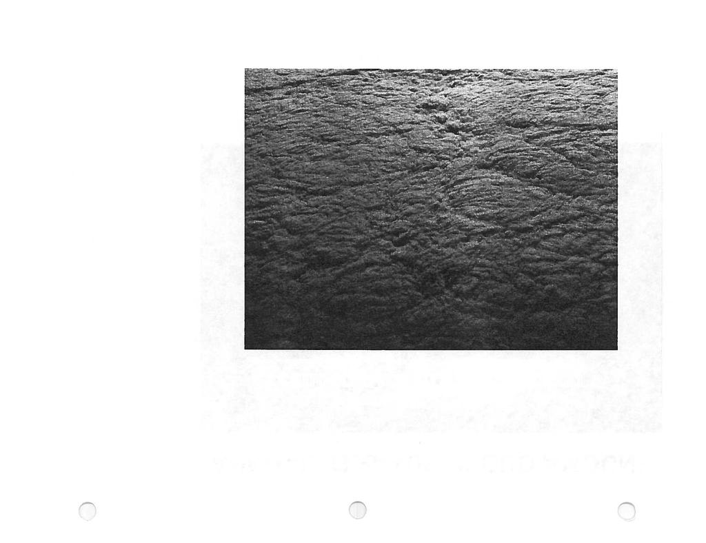
69 Figure 5.1a Figure 5.1b 69

70 Figure 5.2 In the following, I will describe physical processes and observed phenomena within the STBL, discuss some possible mechanisms that dissipate clouds, and show some typical statistical profiles Physical processes The most fundamental physical processes are longwave radiation, turbulence, entrainment, and condensation/evaporation. They exist in all stratocumulus-topped PBLs. In addition, solar radiation can play some role in the daytime, and drizzle is often observed and may also be important in maintaining/dissipating the cloud layer. Longwave radiation cooling at the cloud top Longwave radiation cooling at cloud top exists due to the different radiative properties of water vapor and droplets. In the longwave radiation spectrum, there is a window region where water vapor cannot absorb or emit. But liquid water can absorb or emit at all longwave frequencies. Thus, the downward longwave flux above the cloud 70

71 Figure 5.3 top, which comes from the water-vapor line emission of the overlying water vapor, is smaller than the flux within the cloud layer, which comes from the black-body emission of droplets, as shown in Fig. 5.3a. As a result, the magnitude of the downward flux sharply decreases upward across the cloud top. The upward flux, however, remains quite uniform with height, as shown in Fig. 5.3b, with only a slight change at the cloud base due to the slight difference in temperature at the surface and at the cloud base. The net flux thus has a sharp increase right at the cloud top, and hence strong cooling ( several degrees per hour) occurs over a very thin layer ( 50m) at the cloud top. (Note that the clear-air longwave radiation cooling is only about 1 2 degrees per day, which is two orders of magnitude smaller than cloud-top longwave radiative cooling.) 71

72 Figure 5.4 (SOURCE: Shen and Moeng 1989) When a layer is cooled at the top, downdrafts that carry cooled air parcels are negatively buoyant and hence are accelerated downward. These downdrafts drive turbulence just like updrafts that carry the surface-heated air parcels in the clear CBL case. If the cloud top is a rigid lid, then cooling-from-top should generate turbulence exactly the same as heating-from-bottom CBL case. But the cloud top is a free interface that separates turbulent from non-turbulent air and hence entrainment occurs there. Nevertheless, some similar features were observed between the cooling-from-above and heating-from-below PBLs. For example, Nicholls (1989; QJRMS, 115, ) observed cellular patterns near the cloud tops, with broad updrafts in the centers and narrow downdrafts around the edges. Shen and Moeng (1993; BLM, 65, 29 53) also showed irregular cellular patterns near the cloud tops from their large-eddy simulations, as shown in Fig Turbulent circulations in the cooling-from-top case may not reach all the way to the 72

73 Figure 5.5 surface. For example, in many of Nicholls North Sea cases, circulations reach only to the cloud base, because of the decoupling phenomenon which we will study in section [Notice that the cooling-from-above and heating-from-below concept is different from the top-down and bottom-up diffusion concept that we talked about in section 3. Cooling-from-above or heating-from-below provides the buoyancy force that affects turbulence dynamics. Top-down and bottom-up diffusion in principle applies only to passive scalars that cannot change the dynamics; the top-down/bottom-up diffusion occurs within the same turbulent flow field.] Entrainment Entrainment brings warm and dry air from above into the turbulent layer, and consequently modifies the near-cloud-top cloudy air parcels that are being cooled radiatively. Thus, before those radiatively cooled air parcels go down and buoyantly disturb or drive the flow field, they are modified by entrainment, as sketched in Fig This means that, unlike the CBL, we must know entrainment first in order to know how efficiently cloud-top radiation cooling generates buoyancy and hence turbulence. Because there exists no quantitative understanding of the entrainment processes, modeling the entrainment rate of the STBL remains a problem. Our qualitative understanding of entrainment is the following: Entrainment process depends on turbulence intensity, as well as the inversion strength. The stronger the 73

74 turbulence, the larger the entrainment rate. The stronger the capping inversion, the harder it takes for inversion air to be entrained. The above description may apply well to clear PBLs, but doesn t give the whole picture in determining the entrainment rate in the STBL. This is because cloud-top radiative cooling and entrainment processes interact strongly: More entrainment brings in more warm inversion air, which reduces the efficiency of longwave cooling in driving turbulence; weaker turbulence then in turn weakens entrainment. This is only true if we neglect the condensation/evaporation effect (e.g., a dust or smoke cloud case). With microphysics, the dry air entrained from above can result in another type of cloud-top cooling due to evaporation, as described below. Condensation/evaporation Condensation/evaporation process further complicates the STBL. Condensation occurs in the cloud layer so there typically exists a sharp increase of the buoyancy flux at the cloud base, as we will see in section Near the cloud top, entrainment keeps bringing in dry inversion air, and this yields cooling due to evaporation of cloud droplets. When the inversion air is very dry but not very warm, the evaporative cooling effect dominates the entrainment warming effect, then entrainment can result in net cooling of the near cloud-top air. Under this condition, stronger entrainment gives stronger turbulence, which in turn enhances entrainment. This positive feedback is the so-called cloud-top entrainment instability (CTEI). We will talk about this instability in more detail in section Notice that in the above CTEI argument, we have ignored the radiation cooling mechanism. Solar radiation and drizzle Other processes like solar radiation and drizzle can also play important roles in the stratocumulus-topped PBL, although these processes do not exist all the time. For stratocumulus over the ocean, the influence of solar radiation is from the solar absorption inside the cloud layer, rather than from surface heating and surface fluxes. Unlike longwave radiation, solar heating inside the cloud is more uniformly distributed throughout the cloud layer. The part of heating near the cloud top can offset longwave 74

75 radiation cooling in generating turbulence, while the part throughout the cloud layer directly increases the temperature of the cloudy air. These two effects together can result in a diurnal cycle (which will be mentioned in section 5.1.3) of marine stratocumulus clouds even though the ocean surface temperature remains nearly constant. Furthermore, when the whole cloud layer is warmed by the internal solar heating, the cloud layer may eventually become warmer than the subcloud layer and a thin stably stratified layer may occur at the cloud base. This is one of the mechanisms that is believed to decouple the cloud layer from the influence of the surface. We will talk about decoupling phenomenon next Decoupling Decoupling phenomenon may result from the internal heating of solar radiation in the cloud layer as mentioned above. It can also be due to drizzle. When droplets fall out of the cloud layer, evaporation occurs in the subcloud layer and subsequently cools the subcloud air. When the subcloud air becomes colder than the air in the cloud layer, a thin stably stratified layer may occur somewhere in the subcloud layer, and hence decoupling forms. This drizzle effect has been observed in the field (e.g., Brost et al. 1982, JAS, 39, ; Nicholls 1984, QJRMS, 110, ) and in 1-D closure models (Wang and Wang 1994, JAS, 51, ). Some researchers believe that decoupling is a mechanism that can dissipate clouds. When the cloud layer is decoupled from its underlying surface influence, moisture supply from below is suppressed, and the cloud dissipates. Decoupling phenomenon was first reported by Brost et al. (1982) and Nicholls (1984). Based on aircraft data taken from the North Sea, Nicholls found that the conserved thermodynamic variables, such as equivalent potential temperature or total water mixing ratio, tend to display small discontinuities near cloud base and that the observed buoyancy and total water flux profiles show negative values near the cloud base. Nicholls 1984 paper described many interesting phenomena later observed during FIRE and ASTEX, such as decoupling reported by Betts (1990; Tellus, 42A, ) and drizzle or cumulus cloud forming under the stratiform cloud layer reported by Paluch and Lenschow (1991; JAS, 48, ). On the effects of drizzle, Nicholls stated that The inclusion of precipitation can significantly alter the net transfer of water substance 75

76 Figure 5.6 (SOURCE: Betts 1990) and evaporation below cloud can have a significant stabilizing influence on mixing between the cloud and lower layers. On the decoupling phenomenon, he observed that The cloud and sub-cloud layers are found to be decoupled, i.e., they appear as two separated mixed layers. After decoupling occurs, he found that If the thermodynamic state of the sub-cloud layer subsequently evolves in a manner which enables condensation to occur within it, the resulting cumulus convection may again link the cloud and surface layers. Cumulus rising into stratocumulus is a very common phenomenon... This cumulus-under-stratocumulus phenomenon is illustrated in Fig. 5.6, taken from Betts (1990; Tellus). When stratocumulus cloud is decoupled from the surface influence, cumulus cloud can occur in the lower LCL, beneath the upper LCL where the stratocumulus cloud base is. Since cumulus-under-stratocumulus was a commonly observed phenomenon during the ASTEX field experiment, this phenomenon is believed to be part of the stratusto-cumulus transition process (e.g., Krueger et al. 1995, JAS, 52, ). 76

77 5.1.3 Diurnal cycle Marine stratocumulus cloud undergoes a diurnal cycle even though the underlying ocean surface temperature remains about the same. The diurnal cycle was observed in the 1940 s and modeled by Oliver et al. (1978; JAS, 35, ), and it has gained more attention recently. The cloud layer becomes thinner and its liquid water content becomes smaller in the daytime when the sun heats the cloud layer directly. In addition, the solar heating at the cloud top offsets the longwave radiation cooling there, weakens the buoyancy force that drives turbulence, and hence decreases the moisture supply from the surface to the cloud layer. Sometimes the cloud layer may disappear all together during the day, and reforms at night. The diurnal cycle of stratocumulus over land can be quite different from that over ocean. Over land, the ground can heat up quickly after sunrise due to the part of solar radiation that penetrates through the cloud layer. When the ground heats up, the surface buoyancy flux increases, and the surface sensible heating enhances turbulent transport. If the ground is moist, this enhanced transport can supply more moisture into the cloud layer and therefore helps to maintain the cloud. But if the ground is dry, this enhanced turbulent motion brings warmer air up into the cloud layer, which increases the temperature (and the saturation mixing ratio) of the cloudy air. Thus the change in surface fluxes over land can either thin or dissipate the cloud Cloud Top Entrainment Instability (CTEI) Cloud-Top Entrainment Instability (CTEI) is believed to be a mechanism that breaks up the PBL stratocumulus. This mechanism was first suggested by Lilly in 1968 (QJRMS, 94, ). That classical paper has two very important contributions: It presented the first mixed-layer modeling of the stratocumulus PBL and it is also the first paper proposing CTEI for stratocumulus. I will talk about CTEI next and discuss mixed-layer modeling in section 6. Lilly (1968) argued that when the air above the cloud layer has a smaller equivalent potential temperature than the cloudy air, i.e., Θ e = Θ e (B + ) Θ e (B ) < 0, where B + and B are levels just above and below the cloud top, then any mixture of air from above 77

78 and air inside the cloud will remain colder than the cloudy air. So the mixture can accelerate downward, i.e., becomes negatively buoyant downdrafts, and sink deeper into the cloud layer. This is the so-called CTEI. Randall (1980; JAS, 37, ) and Deardorff (1980; JAS, 37, ) revised this CTEI criterion by considering the effects of liquid water on the buoyancy. From the virtual potential temperature formula shown in (45), we know that q l can modify the buoyancy variable θ v. Based on this definition and other relationships between different thermodynamic variables, Deardorff constructed a buoyancy mixing diagram and used it to demonstrate the CTEI mechanism. Randall, on the other hand, used the flux relationship between buoyancy and conserved variables to demonstrate CTEI. These two different methods ended up with the same conclusion that Θ e has to be much smaller than 0 in order for CTEI to occur. I will use Randall s derivation for illustration. Assuming that after mixing the mixture becomes saturated, then q v = q, where q is the saturation mixing ratio. Since q (T, P ) q (T 0, P ) + ( q ) T p(t T 0 ), q v ( q T )θ cpγ L θ, where γ L c p ( q ) T p. Using the virtual and equivalent potential temperature formulae given in (45) and (46), we can show that the buoyancy flux can be related to the fluxes of the equivalent potential temperature and total water mixing ratio as wθ v (B ) = awθ e (B ) bwq T (B ), (48) where a and b are thermodynamic coefficients for saturated air. Using the jump condition, wθ e (B ) = w e Θ e and wq T (B ) = w e Q T, where w e is the entrainment rate, then (48) becomes wθ v (B ) = w e [ a Θ e + b Q T ]. (49) For the instability to take place, downdrafts (w < 0) have to be negatively buoyant (θ v < 0) such that buoyancy flux near the cloud top remains positive, i.e., wθ v (B ) > 0. Thus, the right-hand side of (49) has to be positive in order for downdrafts to accelerate downward, i.e., Θ e < b a Q T. (50) The right-hand side of (50) is almost always negative and is about 1 3K. If we neglect the liquid water term in the θ v formula (45), the coefficient b in (48) becomes zero and (50) becomes Lilly s criterion. 78

79 Figure 5.7 (SOURCE: Kuo and Schubert 1988) The above CTEI criterion was challenged by observations, however, which often found solid stratocumulus cloud deck under conditions that satisfy the instability criterion (50). The most cited evidence is shown Fig. 5.7, taken from Kuo and Schubert (1988; QJRMS, 114, ); it clearly shows that stratocumulus can still exist when Θ e < 0 (Lilly s CTEI condition) and Θ e < κ L c p Q T (Randall-Deardorff s CTEI condition). Here κ = (b/a)(c p /L). (However, I would like to remind you that in practice it is difficult to define the jump conditions Θ e and Q T because in nature there is often no well-defined mixed layer. Also, soundings often show large variations in these thermodynamic fields just above the cloud top.) Because of the controversy, many studies (e.g., Kuo and Schubert 1988; Siems et al., 1990; QJRMS, 116, ) began to look into more details at the entrainment mixing and evaporation processes involved in the CTEI theory. They used the following thermodynamical analysis to show that not all cloud-top air parcels become saturated after entrainment 79

80 and mixing. Consider a mixture that consists of χ mass units of warm air that is entrained from above and (1-χ) mass units of cool moist air within the cloud layer. The equivalent potential temperature and total mixing ratio of the mixture are (ignore the radiation effect): θ e = χθ ea + (1 χ)θ eb, (51) q T = χq T a + (1 χ)q T b, (52) where the subscript a represents the above-cloud air and b represents the cloudy air. Using the definitions of θ e (Eq. 46), θ v (Eq. 45), and q l = q T q when q T > q, (53) q l = 0 when q T < q, (54) one can then iteratively solve for θ v as a function of χ for given θ ea, θ eb, q T a, and q T b. Figure 5.8 shows examples of four different θ ea, θ eb, q T a, and q T b, with the y-axis showing the buoyancy difference between the mixture air and its unmixed cloudy environment. These four cases have the jump conditions located at points A, B, C, and D, respectively, in Fig The kinks in these four curves at χ = χ indicate the amount of mixing fraction for the mixture to become saturated. Mixtures with χ < χ are saturated and those with χ > χ are unsaturated. 80

81 Figure 5.8 (SOURCE: Kuo and Schubert 1988) Figure 5.8 shows that when the jump condition is on the stable side of the Lilly-Deardorff- Randall curve, such as curve A, all mixtures, with any χ amount, remain warmer than the cloudy (unmixed) environment; none becomes negatively buoyant. When the jump condition satisfies the Lilly-Deardorff-Randall s criterion, curves B, C, and D, some of their mixtures indeed become colder their unmixed cloudy environment, and thus become negatively buoyant (i.e., accelerate downward). However, not all of the mixtures are negatively buoyant; those with larger χ (larger than about 0.15) are still warmer than the unmixed cloudy air. Thus, Kuo and Schubert concluded that the CTEI criterion proposed by Deardorff and Randall is only a necessary, not sufficient, condition for cloud breakup. They also suggested, based on their two-dimensional numerical simulation, that surface evaporation and upward transport processes can apparently provide enough water vapor to compensate for the evaporative effects associated with the weak evaporative instability. Siems et al. (1990) provided a similar interpretation by using the buoyancy reversal concept; buoyancy reversal is a process that after mixing parcels become denser than either of the unmixed fluids, and cannot return to their original place. Parcels experience buoyancy reversal are those having θ v θ vb smaller than zero in Fig Siems et al. defined a D 81

82 value that is the ratio of θ v θ vb at χ (i.e., the most negatively buoyant mixture) and the buoyancy difference between the two unmixed layers, i.e., D = θ v(χ ) θ vb θ vb θ va. (55) Using this definition, Randall-Deardorff s instability criterion is D > 0. (Note that the denominator is negative.) Siems et al. argued that the D value has to be much larger than 0 in order for sustained vigorous mixing (i.e., instability) to occur based on Shy and Breidenthal s (1990; JFM, 214, 1 15) laboratory experiments in a convective tank. The Shy-Breidenthal lab tank consists of two layers of fluids, initially separated by a plate. The lower fluid is denser than the upper one. After a sudden removal of the plate, these two fluids mix nonlinearly and produce mixtures that are denser than either of the two initial fluids. This mixing phenomenon is similar to the mixing of clear and cloudy air; after clear air is entrained into the cloud layer, evaporation occurs, and the mixtures can become denser than either of the unmixed clear or cloudy air. The laboratory results showed that when the buoyancy reversal is relatively large, D > 1.3, the whole system experiences explosive entrainment and becomes unstable, in the sense that the perturbed interface did not relax back to horizontal, but developed a strong tilt. Because of the explosive entrainment, the depth of the lower fluid, h, increases significantly when D > 1.3, as shown in Fig. 5.9, taken from Shy and Breidenthal. 82

83 Figure 5.9 (SOURCE: Shy and Breidenthal 1990) Siems et al. also used a two-dimensional numerical model to simulate the laboratory flow; the numerical results confirmed the laboratory results, as indicated in Fig The entrainment rate of their numerical flows increases significantly only when D > 1.3. For applications, Siems et al. concluded that this large D value is unlikely to occur in the range of hydrodynamic parameters characteristic of mixing at the inversion capping a subtropical stratocumulus cloud layer. Thus it appears unlikely that C(T)EI triggers stratocumulus breakup. However, Siems et al. also recognized the difficulty in defining D or mixing fraction amount from atmospheric sounding, because neither the boundary layer nor the upper-level environment are perfectly well-defined mixed layers as is flow in the laboratory or simulations. Homework 3: A. Derive (48) and show the expressions for a and b. Also estimate the value of κ = (b/a)(c p /L) for typical values of a and b. B. Show that if the q l term in (45) is neglected, then b = 0. [Hint: Use the Clausius- Clapeyron equation T dq /dt = Lq /RT, where c p 1000J kg 1 K 1, L J kg 1, and R 461 J kg 1 K 1.] C. Using the definition of θ v and the equations (51)-(54), plot θ v θ vb as a function of χ 83

84 for θ ea =319.4K, θ eb =316K, q T a =4.5g/kg, and q T b =10.5g/kg and show your result in a plot like Fig Figure 5.10 (SOURCE: Siems et al. 1990) Vertical distributions of turbulence statistics Before I show you some typical profiles of statistics in the stratocumulus-topped PBL, let s see which flux profiles should be linear with height in a horizontally homogeneous, quasisteady state. As in the CBL, we expect the fluxes of conserved thermodynamic quantities to be linear with height under a quasi-steady state. We will use the liquid potential temperature (θ l ) as an example. Total water mixing ratio is also a conserved variable when there is no drizzle. The governing equations for their means are Θ l t = wθ l z 1 ρc p F rad z, (56) and Q T t = wq T z, (57) where F rad is the radiative flux. Taking the z-derivative of (56) and (57) leads to ( Θ l / z) t = 2 wθ l z 2 1 ρc p 2 F rad z 2, (58) and ( Q T / z) t = 2 wq T z 2, (59) 84

85 which should be nearly zero under a quasi-steady state. Therefore the total heat flux, H wθ l + 1 ρc p F rad, and the total water flux, wq T, should remain linear with height if turbulence reaches a quasi-steady state. Since F rad the longwave radiative flux (or longwave plus solar radiative flux in daytime) is not linear with height, the liquid-potential-temperature flux wθ l alone is not linear with height either. When decoupling occurs, turbulence is split to two separate layers and the above argument no longer applies. In this condition turbulent mixing does not extend throughout the whole PBL, H and wq T layers, as suggested by Nicholls. may have two linear curves representing the two separate mixed Profiles of statistics within the stratocumulus-topped PBL vary from case to case, depending on the type of forcing that generates/consumes turbulence. Statistics are different between buoyancy and shear driven PBLs, and also different between cloud-top-cooling driven and surface-heating driven PBLs. When turbulence is driven mainly by cloud-top radiation cooling This type of STBL has been studied the most, observationally and numerically. Typical structure for this type of STBL was reported by Nicholls (1989; QJRMS, 115, ) based on aircraft data taken over the North Sea over solid and horizontally uniform stratocumulus cases, even though most of these cases were decoupled from the surface. The statistics shown in that paper were plotted only for the upper wellmixed layer, i.e., from the cloud top (z /h = 0) down to the bottom of the upper well-mixed layer (z /h = 1) where the cloud-top radiative cooling effect can reach. Thus h here denotes the depth of the upper well-mixed layer, not the whole PBL depth. Nicholls used the following scaling parameters to normalize the statistics: w = [2.5(g/T 0 )h B] 1/3, T = 2.5B/w, and q T = (wq T ) zi /w, where B is the layer-averaged buoyancy flux over the mixed layer h and (wq T ) zi near the cloud top. is the maximum total water flux Figure 5.11a shows the expected linear trend of the total water flux, although the data are quite scattered. Figure 5.11b shows that the maximum buoyancy flux exists at some distance below the cloud top, i.e., at z 0.1h. At z /h = 1 where the decoupling occurred, the buoyancy flux at that level became negative. 85

86 that the fluxes generally decreased downwards and were significantly smaller than w*qt* in the lower part of the mixed layer in all cases except 624, where they were comparable owing to the aforementioned surface transfers (NB. an instrument failure led to the loss of all q data in cloud on flight 624. A value of qt* was therefore obtained by assuming that w4 could be related to in cloud using the saturation condition, as described in NL, which also showed this to be a reasonable - assumption on the other flights. The same assumption was also used when calculating wtv, although the water vapour term is small in this case.) r' A tl t.*? ' A A * T?t t L I I 1 I I I I I I 0 1.o 0 1.o Figure 2. Scaled total water and virtual temperature fluxes v. z'/h. The plotting symbol for each flight is given in Table 1. c C ' -~ Figure 5.11 (SOURCE: Nicholls 1989) The velocity variances shown in Fig are all on the order magnitude of 0.5w 2 with a peak at about 0.8h, close to the cloud top. Nicholls compared his TKE budgets (Fig. 5.13a) with the upside down budgets of a clear CBL (Fig. 5.13b; from Lenschow et al 1980; JAS, 37, ) and those of an LES of STBL (Fig. 5.13c; from Moeng 1986; JAS, 43, ). From Fig. 5.13a and b, Nicholls concluded that the STBL is similar to the upside down version of surface-heated CBL. Unlike the Nicholls s observed case, the LES shown in Fig. 5.13c does not have the decoupling phenomenon, and hence turbulent mixing takes place throughout the whole PBL. Thus, in Fig. 5.13c z /h = 1 is the Earth s surface, whereas in Fig. 5.13a it is a cloud-base level. Because of this difference we may compare them only above z = 0.5h. As pointed out by Nicholls, the overall features between model and observations above 0.5h are similar except the turbulence transport term, T = we/ z. Near the cloud top, observations show large negative, but LES shows a nearly zero T. Between 0.2h < z < 0.5h, T is positive in the observations, but negative in the simulation. The coarse resolution of the LES was first suspected to be the reason for the discrepancy between the observed and simulated T term. But from a much finer 86

87 CONVECTION IN STRATOCUMULUS 491 I..* I T T A '.A.. T T o '. A A Figure 3. Scaled velocity variances and TKE, E, u. z'/h. Symbols as Fig. 2. Figure 5.12 (SOURCE: Nicholls 1989) (c) General characteristics: measured variances The variances measured on each of the selected runs, scaled with the quantities listed above, are shown in Figs. 3 and 4. For conformity with the conditionally sampled data presented in the next section, low frequency variations in all time series have been reduced by removing a 30s (3 km) running mean. The vertical velocity variance reaches a maximum of about 0.4~: in the upper part of the mixed layer, around Z' = 0.2h. Above this, the proximity of the inversion causes a strong decrease. Values above cloud are about an order of magnitude smaller. Significant internal wave activity above cloud top was detected only on flight 511 and the variance is correspondingly higher for this reason. The decrease observed below z' = 0.2h and through the rest of the mixed layer is more 87scattered, reflecting differences in the TKE balance between cases in this region. Case 624 shows no significant variation of with height. A similar plot of the same data in NL showed fair agreement with the results of Lenschow et al. (1980), obtained in surface-heated convective boundary layers, although

88 dissipation in this region in this case, which could support entrainment at the lower boundary. Unfortunately, there are no other observations currently available with which to compare these results. The closest relevant data are those from convective layers over heated surfaces (e.g. Lenschow et al. 1980) and large-eddy simulations (Moeng 1986), although they are not directly equivalent and only limited comparisons are possible. Lenschow et al. obtained their data in cold air outbreaks over a relatively warm ocean surface (plotted upside down in Fig. 17(b) for ease of comparison). The residual term, O- r i' 0.5-2' Figure 17. (a) The composite TKE balance. The terms are described in the text (see Eq. (11)). (b) As (a), but from Lenschow el al. (1980) plotted upside down. Here, the thin full line represents S (see Eq. (11)). the shear generation. (c) As (a), but from Moeng (1986). As in (b), the thin full line represents S. Figure 5.13 (SOURCE: Nicholls 1989) resolution LES (with grid points covering the same domain such that x = y = z = 12.5m), Fig. 5.14, we see that the discrepancy in T term is worse; the fine-resolution LES shows that T is clearly positive near the cloud top. (Compared between the two LESs, the fine-resolution LES has a slightly larger surface heating.) It is clear that the discrepancy in T -term between Nicholls observations and the LES came from the different distributions of w 3. The observed w 3 is negative in the cloud layer and increases to zero at the cloud top: This yields a negative TKE flux we (Fig. 5.15b) throughout the cloud layer for most of the five flight cases. The LES flow, on the other hand, shows a positive w 3 in the cloud layer, which decreases to zero at the cloud top, and a negative w 3 in the lower PBL. The w 3 dominates we, which is then positive in the upper and negative in the lower PBL (Fig. 5.15a; results were from the fine-resolution LES). An explanation for the simulated distribution of w 3 shown in Fig. 5.15a was given in Moeng and Rotunno (1990; JAS, 47, ) based on a direct-numericalsimulation (DNS) study. If there is only surface heating, w 3 and hence the w-skewness 88

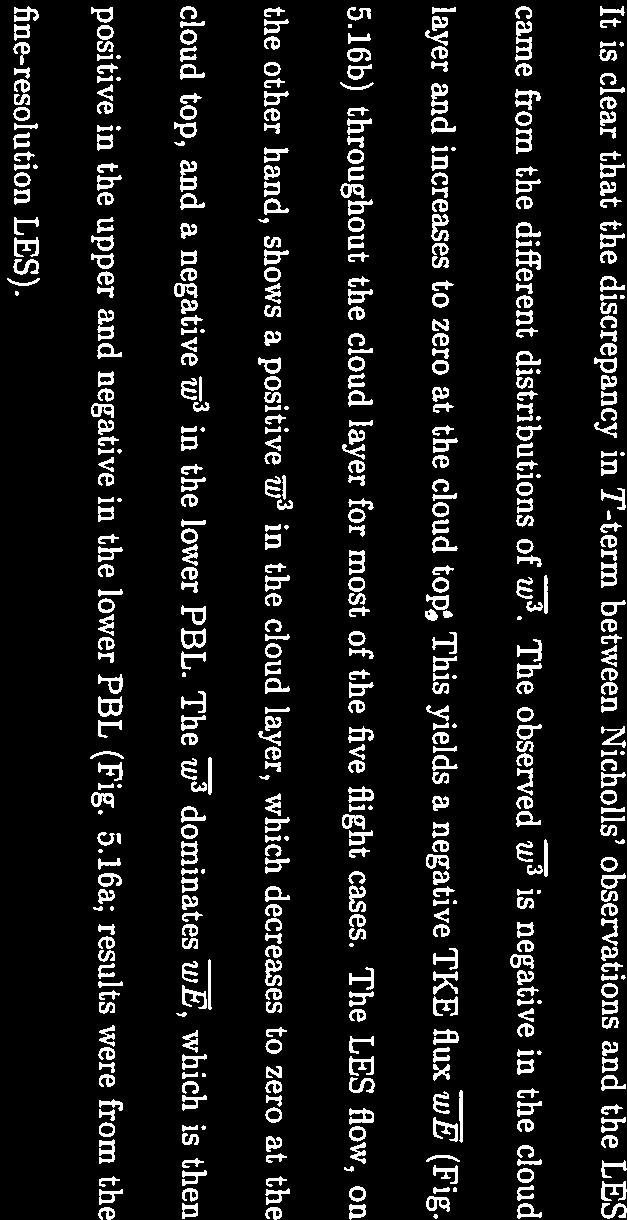
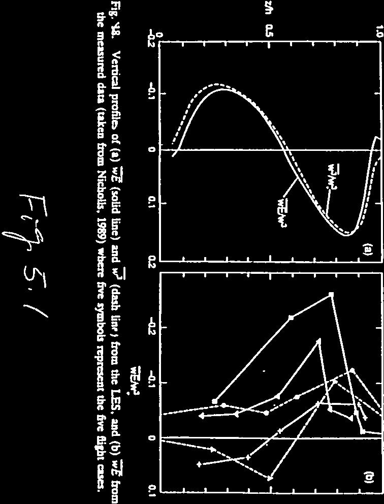
89 Figure 5.14 (SOURCE: Shen and Moeng 1993) Figure 5.15 (SOURCE: Shen and Moeng 1993) 89

90 [ w 3 /(w 2 ) 3/2 ] are positive throughout the whole PBL (just like in the CBL, Fig. 3.9b) because surface-generated updrafts are stronger than downdrafts. Since only few of these strong updrafts can reach to the cloud top, the area coverage by strong updrafts decreases with height. Thus, the largest positive w skewness is likely to occur near the PBL top. Now consider just the effect of cloud-top cooling. Cloud-top cooling generates strong downdrafts, with a few of them reaching all the way to the surface (but only if there is no decoupling). Hence the most negative skewness is likely to be near the surface. Combining the cloud-top cooling and surface heating effects, positive w-skewness occurs in the upper PBL due to surface heating, and negative w-skewness in the lower layer due to cloud-top cooling, just like what we see in Fig. 5.15a. In the observational cases, however, the upper mixed layer was decoupled from its surface influence, so the only buoyancy source that drives turbulence here was cloud-top cooling. Therefore, throughout the whole mixed layer w 3 and hence we are negative. To see if turbulence statistics generated from LES depend sensitively on its numerics, SGS parameterizations, SGS condensation, and/or longwave radiation representations, the GCSS Boundary Layer Cloud Working Group performed its first intercomparison study in The group got together to discuss their results during the 1994 NCAR/GCSS Boundary Layer Cloud Workshop, and the result is summarized in Moeng et al (1996, BAMS, 77, ). An idealized STBL horizontally homogeneous, nearly solid cloud deck, no solar heating, no decoupling, no drizzle, plus negligibly amounts of surface heating and wind shear was chosen to be the first intercomparison case. Ten LES groups participated in this intercomparison study. Although the results vary in magnitude, mainly because the cloud-top radiative cooling amount is different among the LESs as shown later, the vertical distributions of fluxes (Fig. 5.16), velocity variances (Fig. 5.17), and TKE budget (Fig shows the three major terms) calculated from the ten LES codes are quite similar in shape. Figure 5.18a shows that the magnitudes of the buoyancy production vary among the LESs. Comparing Figs. 5.17a and 5.18a, we see that the LESs that have the largest buoyancy production term (e.g., UW) yield the strongest turbulence intensity. 90

91 Figure 5.16 (SOURCE: Moeng et al 1996) Figure 5.17 (SOURCE: Moeng et al 1996) 91

92 Figure 5.18 (SOURCE: Moeng et al 1996) (Note: the UKMO s total TKE is suspiciously large, because both of their horizontal and vertical velocity variances are smaller than those of the UW.) The difference in the buoyancy production term is apparently due to the different amount of cloud-top cooling, which is the main source of buoyancy (and hence turbulence) in this case. The cloud-top cooling rate is an internally determined quantity in LES, calculated from a longwave radiation scheme; different LES codes used different longwave radiation schemes and hence obtained different cloud-top cooling rates (Fig. 5.19). As you can see, the cloud-top cooling rates predicted by the KNMI (diamond-solid line) and UW (open circle-dashed dotted curve) LESs are larger than 4K/hour. Consequently, their buoyancy flux (Fig. 5.16c) and hence the velocity variances (Fig. 5.17; KNMI result is not shown here) are the largest among all LESs. When surface heating also dominates Moyer and Young (1993; JAS, 50, ) analyzed ten FIRE flights, and showed that the buoyancy forcing within the STBL ranged from purely surface forcing to purely cloud-top forcing. Figure 5.20, taken from their paper, shows the variation of the surface heat flux during those ten flights, from slightly negative to significantly positive. When wind shear dominates One of the documented STBLs that were driven by shear was reported by Brost et al. (Part I and II 1982; JAS, 39, and ). They suggested that the 92

93 Figure 5.19 (SOURCE: Moeng et al 1996) Figure 5.20 (SOURCE: Moyer and Young 1993) 93

94 Figure 5.21 (SOURCE: Brost et al 1982) longwave radiative cooling near the cloud top was balanced by entrainment of warm inversion air, and thus produced no impact on mixed-layer turbulence for the cases they analyzed. The mean wind was however very strong, m/s, and the turbulence was driven mainly by shear. In those cases, the liquid water content near the cloud top was very low, 0.1 g/kg. This type of PBLs has a very different structure comparing to buoyancy-driven stratocumulus PBLs. As pointed out by Brost et al., the structure is more like the neutral PBL, where the velocity fluxes and variances scaled well with the friction velocity u, as shown Figs and The temperature and moisture fluxes (Fig. 5.23) obtained by Brost et al. were 94

95 Figure 5.22 (SOURCE: Brost et al 1982) quite complicated. In most cases the total water mixing ratio flux was not linear with height because drizzle occurred. The TKE budget (Fig. 5.24) showed a near balance between the shear production and dissipation, at least in their cases 13-2 and 17-2, which is a feature of neutral, shear-driven PBL. From the above examples (observed and simulated), you can see that the vertical distributions of statistics (such as the buoyancy flux profile) in the STBL vary from case to case; the distributions depend strongly on where and what the dominant turbulence sources (e.g., surface heating, cloud-top cooling and wind shear) are. Therefore, it is unlikely that we can scale the statistics into universal profiles, like we do for the CBL Climate-related issues PBL stratocumulus plays a major role in climate, and hence it is important to accurately represent (parameterize) it in climate models. Randall et al. (1984; BAMS, 65, ) pointed out that a mere 4% increase in the area coverage of marine stratocumulus regime could produce a 2-3 K cooling in the global mean temperature, based on a simple 1-D radiative equilibrium calculation. Such cooling is more than enough to offset the global warming due to doubling CO 2. This sensitivity was also found by T. Slingo (1990; Nature, 343, 49 51) using a 3-D general circulation model. He showed that the net albedo depends 95

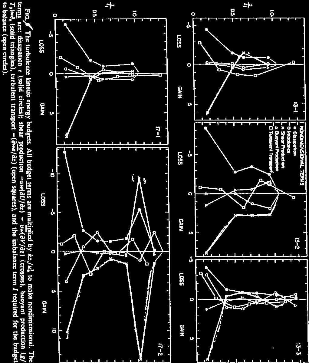
96 Figure 5.23 (SOURCE: Brost et al 1982) Figure 5.24 (SOURCE: Brost et al 1982) 96

97 sensitively on not only the cloud amount but also the details of cloud microphysics near the cloud top, such as the dropsize distribution. Not knowing how to accurately represent these cloud properties of the marine stratocumulus poses a big challenge in predicting climate changes. To develop such a parameterization, we need to put our qualitative understanding of the cloud regime (described in early subsections) into quantitative forms. This is a difficult task, however, because as we have learned that there are many physical processes involved and all of them can play an important role in determining the cloud properties. One way to pursue this problem is to consider just a few dominant physical processes to see if we can express the turbulent fluxes and the cloud properties as functions of large-scale forcing and sounding. For such a study, we may ignore the solar radiation (and drizzle) and consider just some basic physical processes like longwave radiation, entrainment, turbulent transport, and condensation/evaporation. But if one is interested in the direct impact of this cloud regime on climate, one needs to include solar radiation because the direct impact of stratocumulus is due to its much larger cloud albedo than the ocean surface s. Current GCMs use very simple cloud schemes to represent the marine stratocumulus. The majority use an empirical cloud scheme developed by J. Slingo (1987, QJRMS, 113, ), in which the cloud fraction depends on large-scale quantities like stability in the lower atmosphere (i.e., the inversion strength) and the relative humidity in the PBL. The scheme was developed based on climatology data and is purely empirical. One of the deficiencies of such a scheme is that the cloud field is not directly linked to the turbulence and radiation fields. In fact, most GCMs treat these three fields (turbulence, radiation and cloud) separately by using three separately developed schemes; the only link among these processes is through the large-scale mean field. As we have learned, these physical processes are strongly coupled on turbulence time scale, so they should be treated as a whole system in climate models. The only GCMs that directly link these processes are the ones that use mixed-layer models, developed by Randall and his UCLA/CSU colleagues (Suarez et al. 1983, MWR, 111, ; Randall et al 1985, JAS, 42, ), but in that type of modeling there are complicated closure problems (such as entrainment-rate closure) to deal with. 97

98 Finally, I would like to point out that most stratocumulus studies have been focused on cloud breakup mechanisms, e.g., decoupling, CTEI, stratus-to-cumulus transition; very few on formation processes. Before cloud forms, there is no cloud-top longwave cooling to drive the boundary-layer turbulence. And since most cloud regime exists over cold ocean surface, there is not much surface heat flux to generate turbulence either. How then is the moisture being transported upward to form cloud? One possibility is that this cloud regime, at the very upstream region, may form as fog, and then longwave radiative cooling occurs at the fog top, which drives turbulence; with more turbulence and entrainment the fog then evolves to an elevated cloud as it moves downstream. Another possibility is that the wind shear is strong in this upstream region to driven enough turbulence to carry moisture up to the lifting condensation level, then cloud forms. Without knowing what mechanism drives turbulence to form cloud, it is difficult to come up with a parameterization scheme for cloud formation. 5.2 Shallow cumulus Shallow cumulus clouds occur often over the tropical and subtropical oceans. In the 70 s when aircraft observationalists were searching for horizontally-homogeneous, quasi-steady state PBLs, they naturally went out to the tropical oceans to collect such data. Among those datasets were the Puerto Rico cases reported in e.g., LeMone and Pennell (1976; MWR, 104, ) and the GATE data analyzed by e.g., Nicholls and LeMone (1980; JAS, ). A shallow-cumulus-topped PBL is often found to have a three-layer structure, as first observed by Malkus (1958; Papers Phys. Oceanogr., 13, 47pp): subcloud mixed layer, cloud layer, and the in-between transition layer, as sketched in Fig The transition layer is defined as the upper part of the mixed layer where entrainment effect is significant. Note that, unlike stratocumulus, cumulus clouds exist in a stably stratified environment, and their surrounding air is not very turbulent Interaction between cloud and subcloud layers Among the three Puerto Rico cases they analyzed, LeMone and Pennell (1976) characterized two types of shallow cumulus clouds, that occurred in suppressed convective conditions, 98

99 Figure 5.25 e.g., their Cases I and II, and that in more enhanced convection conditions, e.g., Case III. The difference between suppressed and active cumulus clouds was shown in their schematic diagram, Fig In suppressed conditions, cumulus clouds formed at the tops of rising thermals from the mixed layer that penetrate into the condensation level. In Puerto Rico Cases I and II rising thermals were carried upward in the rising branches of 2-D roll vortices. This type of cumulus clouds is passive, and is like those described as forced cumulus clouds in Stull s book. These clouds are more likely to organize in lines, in the form of roll vortices. They do not dynamically alter subcloud layer. For more enhanced cumulus convection, as in Case III, clouds were found to strongly interact with subcloud layer. This type is described as active cumulus clouds by Stull. These clouds are positively buoyant and the associated pressure fields may produce strong updrafts near the cloud base to suck up mixed-layer air into cumulus clouds (LeMone et al. 1988, MWR, 116, ). These updrafts were traceable to at least 100m below cloud base, according to LeMone and Pennell Subcloud-layer spectra and statistics Figure 5.27, taken from LeMone and Pennell, shows the wavelengths of spectral peaks in the u, v, and w wind fields, which represent the dominant eddy sizes, within the subcloud layer. Roll scales were observed in Cases I (diamonds) and II (circles), as seen in the v 99

100 Figure 5.26 (SOURCE: LeMone and Pennell 1976) 100

101 (or u) spectrum, but less in the w spectrum since random turbulent motion dominates the w-spectrum. Convective roll vortices were not observed in Case III (triangles). Dominant turbulent eddies shown in the w spectrum increased nearly linearly with height to 0.5z i. Figure 5.27 (SOURCE: LeMone and Pennell 1976) The GATE aircraft data reported in Nicholls and LeMone (1980) were mostly under suppressed convective conditions and had much weaker winds than the Puerto Rico cases. 2-D roll vortices were not common there. Figure 5.28 shows that the peak wavelengths in the w-spectrum in the cumulus-topped mixed layer over the ocean had a similar distribution to, but larger in size than, those of CBLs over land reported by Kaimal et al. (1976). (Note that Kaimal et al. spectra were obtained from tethered balloon data, and hence should 101

102 Figure 5.28 (SOURCE: Nicholls and LeMone 1980) be compared with the alongwind aircraft data as shown in Fig. 5.28a.) In the moisture spectrum, Fig. 5.29, no clear dominant eddy size was found; fluctuations of the order of 10 km in scale often occurred and even dominated the spectrum. However, these large-scale bands carried very little moisture flux, as shown by the peaks in the w q cospectra, Fig. 5.30, taken from Nicholls and LeMone. The horizontal structure of these large-scale fluctuations were constructed by LeMone and Meitin (1984; MWR, 112, ), using several parallel flight legs at z =150m, shown in Fig The cloud base height in these cases was about 600m. There were clearly mesoscale band structures. LeMone and Meitin found that these bands were aligned with subcloud- 102

103 Figure 5.29 (SOURCE: Nicholls and LeMone 1980) 103

104 Figure 5.30 (SOURCE: Nicholls and LeMone 1980) 104

105 Figure 5.31 (SOURCE: LeMone and Meitin 1984) layer shear and traveled in a direction of the subcloud-layer wind. Thus, they concluded that this 2-D structure is primarily subcloud-layer phenomena. The horizontal:vertical aspect ratios of these mesoscale bands are on the order of 25 50, similar to 3-D mesoscale cellular convection (i.e., open and close cells). These mesoscale organizations have a much larger aspect ratio than the 2-D roll vortices or 3-D irregular hexagonal convections we mentioned in section 3, which are scaled with z i, i.e., aspect ratio 1. What causes the large aspect ratio, either in 2-D or 3-D form, remains an interesting research topic. One hypothesis is that the structures resulted from modulation of the PBL by tropospheric gravity waves, which themselves may have originated from clouds, as discussed by Clark, Hauf, and Kuettner (1986; QJRMS, 112, ). A numerical simulation by Balagi et al (1993; JAS, 50, ) produced observed cloud structures, i.e., similar orientation and wavelengths. The large eddy simulation method was used to simulate the Puerto Rico cases by Sommeria and LeMone (1978; JAS, 25 39), and then recently by Cuijpers and Duynkerke (1993; JAS, 50, ) and a BOMEX case by Siebesma and Cuijpers (1995; JAS, 52, ). Most of the fluxes or variances obtained from those simulated fields agreed quite well with 105

106 Figure 5.32 (SOURCE: Nicholls and LeMone 1980) observations. The KNMI (Siebesma et al.) has been using their LES solutions as database to develop mass-flux parameterizations of cumulus for GCMs. I also show the GATE observations: mean fields in Fig moisture variance in Fig. 5.33, and the temperature and moisture fluxes in Fig. 5.34, taken from Nicholls and LeMone (1980). The subcloud layer was well mixed. As indicated in the moisture variance profiles, the upper part of the mixed layer was strongly affected by entrained dry air from above. Figure 5.35 showed that wt and wq at the cloud base varied among different cases, while wt v at the cloud base remained nearly zero. This led Nicholls and LeMone to conclude that the sensible and latent heat fluxes at the top of the mixed layer (and therefore the distribution of heating and moistening in the boundary layer) are strongly affected by the presence or absence of cumulus convection while the virtual heat flux remains unaffected. Another interesting study in the Nicholls and LeMone paper is on the convective mass flux, which is a closure in mass-flux modeling as we will learn in section 6. In mass flux modeling, the vertical flux of any scalar c is expressed as wc = ω c (C U C D ), (60) 106

107 Figure 5.33 (SOURCE: Nicholls and LeMone 1980) Figure 5.34 (SOURCE: Nicholls and LeMone 1980) 107

108 Figure 5.35 (SOURCE: Nicholls and LeMone 1980) where ω c σ(1 σ)(w U w D ) is a convective mass flux; σ is the area covered by all updrafts; w U and w D are averaged vertical-velocity speeds within updrafts and downdrafts, respectively; and C U and C D are averaged concentrations of c within updrafts and downdrafts. Another way to write (60) is wc = ω (C U C). (61) C is the averaged concentration over the whole horizontal plane, i.e., over both updraft and downdraft regions, defined as C = σc U + (1 σ)c D. ω σw U is also a convective mass flux. Nicholls and LeMone used the GATE data, which gave the fluxes shown in Fig and the differences (q U q), (T U T ), and (T vu T v ) shown in Fig. 5.35, to compute ω ; their results are shown in Fig Nicholls and LeMone noted that the mass flux at the cloud base was only a small fraction of that in the middle of the mixed layer. Nevertheless, this small amount of cloud-base mass flux ( 0.1ω /w ) produced large fluxes of sensible temperature and moisture there, because T U T and q U q were large at the cloud base. Note that the vertical distribution of this mass flux was similar to the profile of standard deviation of vertical velocity shown in Fig. 5.37, so we may assume that ω σ w ; they are both larger at the cloud-base level when clouds are present at the top of the mixed layer, compared to the clear CBL. This provides important information for mass flux modeling, as we will see in section

109 Figure 5.36 (SOURCE: Nicholls and LeMone 1980) Figure 5.37 (SOURCE: Nicholls and LeMone 1980) 109

110 5.2.3 Climate impact Trade-wind cumulus plays an important role in transporting moisture from the ocean surface to the lower troposphere, which is then advected to the ITCZ to supply the moisture to deep convection. Recently, the KNMI research group (e.g., Siebesma and Cuijpers 1995; JAS 52, ; Siebesma 1997; NATO ASI Series on Buoyant Convection in Geophysical Flows, Kluwer Academic Publishers, 491pp) has been using LES as database to develop mass flux parameterizations of trade cumulus for GCMs. For such a development, some basic questions need to be answered first. For example: What determines the mass flux from the mixed layer into cumulus clouds? How does the cumulus ensemble affect the mixed-layer turbulence? How to parameterize the later mixing between the cumulus ensemble and its environment? 110

111 6 PBL MODELS (PARAMETERIZATIONS) PBL modeling (or called PBL parameterization) is an attempt to describe the statistical behavior of PBL turbulence through simplified equations or modeling frameworks. We can parameterize PBL turbulence in a climate or weather forecast model because its time scale is much shorter than the time scale of large-scale variation. Thus we can assume that turbulent flow responds to large-scale forcing almost instantaneously and that its statistics remain at an equilibrium state for a given large-scale environment. A PBL model is usually designed to provide the following statistical information to a large-scale model: the PBL depth, surface stress, surface fluxes of heat, moisture and other species, vertical profiles of these fluxes within the whole PBL, and cloud amount, if the large-scale condition favors low-level clouds. The surface fluxes are needed to couple the atmosphere with the land processes, the vertical profiles of fluxes determine the time-rate-of-changes of wind speed, wind direction, temperature, and moisture, etc., and cloud amount determines the amount of radiation in/out of the Earth s surface. Therefore all meteorological forecast models need a PBL model. We may categorize all existing PBL models into six different frameworks: Higher-order closure model, Richardson-number-dependent K approach, K-profile model, mixed-layer (bulk) model, transilient theory/integral closure model, and mass flux model. As we will learn next, some models are more elegant and sophisticated than others, but as John Wyngaard stated, they don t necessarily perform better than simple models. As John put it: The key to PBL model performance is not its framework, but calibration against data. It is also important to note that all schemes are just an attempt to describe complicated turbulence processes with a simple set of equations or frameworks. We should never expect any of them to work perfectly. As Lumley stated, these models at their best produce only likenesses of turbulence, and work only in a limited range about their calibration state. Some PBL models are developed for or calibrated against shear-driven turbulence, and others are for buoyancy-driven turbulence. 111

112 6.1 Higher-order closure model (or single-point closure) Higher-moment equations and closure problems Higher-order closure modeling began in the 1970s when researchers found that simple eddy diffusivity (K) models failed to properly represent the PBL turbulence, especially the buoyancydriven turbulence, and also because computers became more powerful. This turbulence modeling approach carries prognostic equations for higher-moment statistics. The idea behind this approach is that if a crude assumption for second moments predicts first moments adequately, perhaps a crude assumption for third moments will predict second moments adequately (Lumley and Khajeh-Nouri 1974; Advances in Geophysics, 18A, ). The hypothesis is that if you solve higher moment equations where you make closure assumptions, you are likely to get a better mean (first-moment) field. There is no prove to this hypothesis, however. Higher-order closure modeling is sometimes referred to as single-point closure modeling because the statistics it predicts are correlations at the same location, e.g., u (x i )w (x i ). All of the moments equations can be derived from the equations of fluctuations u, v, and w, Eq. (1-9). For example, equations for u 2, v 2 and w 2 are: u 2 t = wu2 2uw U z z 2u p x ɛ u, (62) v 2 t = wv2 2vw V z z 2v p y ɛ v, (63) w 2 t = w3 z + 2 g Θ 0 wθ 2w p z ɛ w, (64) where on the right-hand sides are turbulent transport, mean shear (or buoyancy) production, pressure effect, and molecular dissipation terms. Here we applied the PBL assumption so the x and y derivatives of all statistics are set to zero. The sum of these three equations yields the equation of the turbulent kinetic energy, E (u 2 + v 2 + w 2 )/2. Similarly, we can derive all third moment equations, such as those for u i u j u k or we. Higher-moment equations are formally derived from the fluctuation equations without any assumptions; each terms in the budget have its physical meanings. This makes the 112

113 higher-order closure approach very attractive and popular in the 70s and early 80s. It was considered elegant and sophisticated. However, through such derivations, the budget (right-hand side) of every higher-moment equation always consists of one or more higher moment terms. For example, in the secondmoment equation for u 2 i, a third-moment term wu 2 i appears on the right-hand side. Thus, to solve the second-moment equations, one has to (1) make closure assumptions that relate wu 2 i to lower moment (second or first) statistics, or (2) carry prognostic equations for wu 2 i make closure assumptions on the 4th-moment terms. The first approach is called secondorder closure modeling, and the second approach is 3rd-order closure modeling. For 3rdorder closure modeling, we can use a well-established turbulence theory, called quasi-normal (or called quasi-gaussian) approximation, to relate fourth moments to second moments as abcd = ab cd + ac bd + ad bc, which is more accurate than the downgradient assumption (described later) used in the second-order closure modeling. But a 3rd-order closure modeling requires solving many more prognostic equations. For a cloudy PBL, Moeng and Randall s (1984; JAS, 41, ) 3rd-order closure model carries 31 more prognostic equations than a 2nd-order closure model. If one stays with the second-order closure approach, as most PBL modelers do, then closure assumptions are needed for third-moment turbulent transport, pressure-related terms, and molecular dissipation terms, e.g., 1st, 3rd, and 4th terms on the right-hand sides of (62), (63), and (64). The basis of making closure assumptions is well described in Donaldson (1973; Workshop on Micrometeorology, Ed. D.A. Haugen, AMS, ). Each closure formula has to a) be invariant under both coordinate and Galilean transformations, b) have the right dimensional properties on both sides of the formula, and c) satisfy all the conservation relationships known to govern the variables in question. For example, a third moment term, u i u j u k, can be expressed as u i u j u k x i u j u k + x j u i u k + and x k u i u j, (65) in order to be invariant under coordinate transformation. To have the same dimensions on both sides of the formula, we must have u i u j u k λq[ x i u j u k x j u i u k + x k u i u j ], (66)

114 where λ is a characteristic length scale and q is a characteristic velocity scale. The minus sign is added to insure that turbulent energy is diffused down the gradient. This is the wellknown downgradient diffusion assumption. As we will see later, however, this assumption is inappropriate for buoyancy-driven turbulence. Molecular dissipation terms are typically written as a decay form, for example, ɛ ui = ν u i x i u i x i u2 i Λ (67) in the u 2 i equations, where Λ is a dissipation length scale. Pressure fluctuations act to return the turbulent motion to an isotropic state, which can be understood from the following analysis: The pressure terms in (62)-(64) can be re-written as p u i = u ip + p u i, (68) x i x i x i where the first term is a transport. The second term on the right-hand side of (68) drops out of the TKE equation, since p u i / x i =0 for incompressible fluid. But each individual component, p u/ x, p v/ y or p w/ z is not zero. So such pressure-related terms do not generate turbulent energy; they only redistribute energy among u 2, v 2, and w 2 components. For example, in buoyancy-driven turbulence, buoyancy [2nd term in (64)] produces w 2 and through the pressure effect w 2 energy is redistributed to u 2 and v 2. In shear-driven turbulence, the along-shear energy is gained directly from the shear production [2nd term in (62) if U is the streamwise component], then pressure fluctuations redistribute it to v 2 and w 2. Hence, this term generates the return-to-isotropy effect first discussed by Rotta in Thus, in general the pressure terms u i p/ x j are often expressed as u i p x j u j p x i = 1 τ (u iu j 2 3 δ ije), (69) where τ is the return-to-isotropic time scale. This pressure closure includes only the nonlinear turbulence-turbulence interaction, which is referred to as the slow part of pressure effect. To include the direct effects of mean shear and buoyancy, rapid parts should be added to the closure formula (69); for example, the rapid part of pressure closures due to mean shear takes the form of U i / x j and U j / x i (e.g., Launder, et al., 1975; J. Fluid Mech., 68, ) and that due to buoyancy takes the form of 114 g Θ 0 θc in the budget of wc (Moeng and

115 Wyngaard 1986; JAS, ). The contribution from the rapid part can be as large as that from the slow part. Under the PBL assumption, the transport term, first term in (68), is zero in the u 2 and v 2 equations; the only pressure transport term shows up after summing up all three velocityvariance components is wp, as shown in the TKE equation (derived in Homework 1C, z Section 1.3). This transport term is neglected under the closure assumption (69). But as we showed in Fig this pressure transport term can be large in the buoyancy-driven PBL The Mellor-Yamada model In early 70s, Mellor and Yamada realized that it was too computationally costly in a GCM or mesoscale model to use a full set of second-order closure model. They developed a hierarchy of models for the PBL where they systematically reduced the set of equations using a nondimensional measure of anisotropy, a a ij, where u i u j = (δ ij /3 + a ij )u 2 i (Mellor and Yamada 1974; JAS, 31, ). This hierarchy is summarized below. Level 4 All second moment are solved with full equations Let advection and turbulent transport=o(a) and neglect O(a 2 ) terms Level 3 Only TKE and θ 2 are solved with full equations Let advection and turbulent transport=o(a 2 ) and neglect O(a 2 ) terms Level 2 All second moment equation are reduced to algebraic forms Neglect all O(a) terms Level 1 All second moment equation are reduced to algebraic forms The so-called Level 4 model is a full second-order closure model, which solves for the full set of prognostic equations of all second moments. Level 3 neglects all the time-rate-ofchange and turbulent transport terms except those in the equations of TKE and temperature variance (θ 2 ). Level 2 further neglects the time-rate-of-change and turbulent transport terms in the TKE and the θ 2 equations. Hence in Level 2, all second-moment equations reduces 115

116 to a set of simplified diagnostic (algebraic) equations; one can analytically solve that set of algebraic equations, which leads to the following flux-gradient relationships: and uw = K M U z, (70) vw = K M V z, (71) wθ = K H Θ z, (72) where K M = lqs M (R i ) and K H = lqs H (R i ), where l and q are length and velocity scales (to be defined later) and R i is the Richardson number. Thus, Level 2 looks like a Richardsonnumber-dependent eddy diffusivity model (to be described next), except that their K M and K H are formally derived from a set of moment equations, rather than determined empirically. Level 1 has K M and K H similar to those in Level 2 but is seldom, if ever, used. The most popular higher-order closure scheme used in GCMs or mesoscale models is Level 2.5, which is an intermediate version between Level 2 and Level 3; it makes a further simplification to the Level 3 model so that the only full prognostic equation retained is the TKE equation. The Mellor-Yamada Level 2.5 model, also called TKE model or known to the engineering community as a One-Equation Model, is described in Mellor and Yamada (1982; Rev. Geophys. Space Phys., 20, ) and briefly summarized below. E t = z [5 3 qλ E U 1 ] uw z z vw V z + g Θ 0 wθ ɛ, (73) where the first term on the right-hand-side comes from the downgradient assumption for the sum of the turbulence and pressure transport terms. The length scale is empirically set to λ l, where l is a master length scale defined later. The fluxes uw, vw and wθ are calculated from their algebraic equations. The molecular dissipation term is parameterized as where the dissipation length scale is empirically set to Λ 1 15l. ɛ = q 3 /Λ 1, (74) The most difficult and uncertain part of the higher-order closure approach is in determining the characteristic scales of length and time (i.e., l, and τ) that appear in the above closure 116

117 formulae. These scales are supposed to represent the net effect of all turbulent motions large and small eddies and thus depend strongly on the type of turbulent flow fields. [For comparison, the characteristic length scale in the subgrid-scale model in LES is supposed to represent the local-equilibrium inertial subrange eddies, and thus can be more reasonably and universally described by the effective grid size of LES.] In Mellor and Yamada s hierarchy models, all length scales (such as Λ 1 and λ 1 ) are assumed to be proportional to a master length scale, l. The early version of Mellor-Yamada models used a length scale proposed by Blackadar (1962; J. Geophys. Res, 67, ) as κz l =, (75) 1 + κz/l 0 where l 0 is an asymptotic value given as zi 0 l 0 = α qzdz, (76) qdz zi 0 where z i is the PBL height, q = 2E, α is a proportionality constant to be determined (or calibrated) empirically. The newer version of Mellor-Yamada models uses an alternative method for the master length scale (Mellor and Yamada 1982; Rev. Geophys. Space Phys., 20, ), in which a prognostic equation for q 2 l is solved; along with the equation for the TKE, the master length scale l can be retrieved. All time scales are then related to the length and velocity scales as τ l/q. In recent years, many turbulence researchers, particularly within the engineering community, have become critical to the second-order closure approach. They questioned the accuracy of the second-order closure modeling and argued that it is no longer needed for the development of second-order models because with the increase of computer power DNS and LES can explicitly calculate the turbulent motion, which represents turbulence more accurately. An interesting debate on this issue is given in Lumley (1990; Whither Turbulence? Turbulence at the Crossroads, Lecture Notes in Physics, vol. 37, Springer-Verlag). For the meteorology community, however, LES remains too costly to substitute for ensemble-mean closure model in representing the PBL in GCMs or mesoscale models Realizability issue Solving moment equations with ad hoc closure assumptions for higher moment terms often leads to undesirable realizability problems, such as generating negative variances or quantities 117

118 not satisfying the Schwarz s inequality. These problems were first discussed in Schumann (1977, Phys. Fluids, 20, ) and Lumley (1979, Adv. Appl. Mech., 18, ). The crudest way to handle realizability problems is by imposing the clipping approximation as proposed by Andren et al (1976, JAS, 33, ), where the predicted variances are set to zero if they become negative and the Schwarz inequality is imposed for all predicted quantities. There were more sophisticated methods to handle the realizability issue (e.g., Galperin et al. 1988, JAS, 45, 55 62), but it remains one of the critiques of the higher-order closure modeling Applications to cloud-free PBLs The Mellor-Yamada second-order closure models are well documented in the PBL literature, and perhaps the most popularly used PBL schemes. Among the series of papers published by Mellor and Yamada, Mellor (1973; JAS, 30, ) showed that the second-order closure modeling, when applied to the surface layer, was able to reproduce Monin-Obuhkov similarity functions. Yamada and Mellor (1975; JAS, 32, ) showed that this closure model can properly produce the diurnal cycle of mean fields of the Wangara data, as shown in Fig More applications are described in Mellor and Yamada (1982; Rev. Geophys. Space Phys., 20, ). Although Mellor-Yamada models can produce well some mean fields of the PBL, the TKE budget computed from their Level 4 model (top panel in Fig. 6.2) shows unrealistic features compared to observations and LESs (bottom panel in Fig. 6.2, from Moeng and Wyngaard; 1989, JAS, 46, ). The modeled entrainment flux of potential temperature (i.e., wθ at the PBL top) is nearly zero, instead of 0.2 of its surface value. In fact, this model underestimates the entrainment fluxes of all variables. Also, the third-moment turbulent and pressure transport terms (labeled as Diffusion in Fig. 6.2) are greatly underestimated. In Section 6.1.6, we will examine the closure assumptions used by Mellor-Yamada, which will show why the TKE budget resulted from that model is unrealistic. Because of its complexity, the second-order closure model developed by Lumley and his colleagues was rarely used in the PBL community except some earlier works by Wyngaard et al. (1974; Adv. Geophys. 18A, ) and Zeman and Lumley (1976; JAS, 33, ). Their closure schemes include more physics and hence are a lot more complicated 118

119 Figure 6.1 (SOURCE: Yamada and Mellor 1975) and computationally expensive than the Mellor-Yamada s. This model, however, is shown to predict much reasonable entrainment fluxes, e.g., the entrainment flux of buoyancy as shown in Fig. 6.3; that success will be explained in Section Note that Zeman-Lumley s model also predicts a reasonable vertical distribution of the TKE flux, we (Fig. 6.4) for the buoyancy-driven PBL, and consequently a reasonable turbulent transport term (which is we/ z) in the TKE budget. Second-order closure modeling has also been applied to the stably stratified PBL. In Wyngaard (1975; BLM, 9, ), a full second-order closure model was used to model a stable PBL and the results agreed well with observations. Figure 6.5 compares the time evolution of the calculated and observed (a) friction velocity (i.e., r.m.s. of surface momentum fluxes), (b) surface heat flux, and (c) PBL height. Brost and Wyngaard (1978; JAS, 35, ) further simplified Wyngaard s full second-order closure model to a K-type model by neglecting the time-rate-of-change and turbulent transport terms. (For stable or neutral PBLs, we have learned that the turbulent transport terms are typically much smaller than the production and dissipation terms in the 119

120 Figure

121 Figure 6.3 (SOURCE: Zeman and Lumley 1976) Figure 6.4 (SOURCE: Zeman and Lumley 1976) 121

122 Figure 6.5 (SOURCE: Wyngaard 1975) TKE budget.) Also, instead of solving a prognostic equation for the molecular-dissipation rate, they parameterized the length scale as where l B is given as l = l 2 B = z 1 + z/l B, (77) w2 g Θ T 0 z, (78) which came from the assumed balance between inertial forces ( w 2 /l B ) and buoyancy forces [ (g/t 0 )( Θ/ z)l B ]. Thus, l z near the surface, which is a well-known surface-layer property, and l l B in the upper part of the stable PBL. This much simplified second-order closure scheme was shown to reproduce all turbulence results obtained in Wyngaard (1975). This is perhaps not surprising because we showed that eddies within the stably stratified PBL are small and turbulent mixing is more or less local. Thus, a simple K model with a proper length scale as given in (77) and (78) can model the stable PBL well. 122

123 6.1.5 Applications to stratocumulus-topped PBL To apply the second-order closure approach to the stratocumulus-topped PBL, we need to make some modifications: Instead of using θ (or θ v ) and its related moment statistics as prognostic variables, we should use thermodynamic variables that are conserved under moist adiabatic processes, e.g., θ e (or θ l ) and its related statistics. Only conserved quantities can become well mixed by turbulence. The buoyancy (or liquid water) statistics are then computed from the predicted statistics through thermodynamic relationships, e.g., wθ v = awθ e + bwq T, where the coefficients a and b differ for unsaturated and saturated air. In partly cloudy region, which is often the case in a GCM grid, buoyancy statistics can no longer be easily related to the conserved thermodynamic statistics (see Randall 1987; JAS, 44, ). This remains a research problem. For modeling the cloud-top PBL, we also need to add the radiation effect into the mean equation of θ e or θ l, especially longwave radiation cooling at the cloud top because it provides the major source in driving/maintaining the turbulent motion, as discussed in Section 5. For cloudy PBLs, in addition to the vertical fluxes of momentum, heat, moisture or other scalars, turbulence statistics, such as temperature and moisture variances and covariance (θe, 2 qt 2, and θ e q T ) may also be important. According to Sommeria-Deardorff s (Sommeria and Deardorff 1977; JAS, 34, ) subgrid-scale condensation scheme, these statistics determine the cloud amount and cloud fraction within, say, a GCM grid. This becomes one of the advantages of using higher-order closure modeling because other PBL models do not attempt to model these thermodynamic statistics Examination of closure assumptions and constants In the above-mentioned closure assumptions, many closure constants are left to be determined empirically. Traditionally, wind tunnel (i.e., pure shear-driven) turbulence data were used to calibrate those constants. However, shear-driven turbulence is quite different from buoyancy-driven turbulence, and hence any closure that was tuned to shear turbulence is unlikely to work well for convective turbulence. An alternative is to use large-eddy simulation flows as database to calibrate closure assumptions (or constants) for buoyancy-driven PBLs. I will show some examples below. 123

124 Pressure-scalar covariance A closure problem for the pressure-scalar covariance term, 1 ρ 0 c p/ z appears in the scalarflux equation: wc = w2 c C w2 t z z + g θc 1 c p T 0 ρ 0 z, (79) where c is a scalar. To examine such closure, Moeng and Wyngaard (1986; JAS, 43, ) divided the pressure fluctuations into five components, p T, p S, p B, p C, and P SG, according to the four physical processes that appear on the right-hand side of the pressure Poisson equation, 1 2 p = ( V ρ 0 x u i ) 2( U w i z x + V z w y ) + g θ T 0 z + f( u x v ) + SGS, (80) y plus the subgrid-scale contribution in LES. The five components are defined as: 1 2 p T = ( V ρ 0 x u i ), (81) i 1 2 p S = 2( U ρ 0 z w x + V z w ), (82) y 1 2 p B = g θ ρ 0 T 0 z, (83) 1 2 p C = f( u ρ 0 x v ), y (84) 1 2 p SG = 2 τ ij, (85) ρ 0 x i x j where p T comes from the nonlinear turbulence-turbulence interaction, p S from mean shear, p B from buoyancy, and p C from Coriolis term. Separating the total pressure fluctuations into five components makes it easier to formulate closure hypothesis for each component, as we can see in the following. For example, for the buoyancy effect, we Fourier-transform (83) to κ2 p B (κ) = g (iκ z ) θ(κ), (86) ρ 0 T 0 where i = 1, and represents quantities in Fourier space. Dividing both sides by κ 2, multiplying by iκ z and the complex conjugate of c, and then Fourier transforming the equation back to the physical space, we obtain 1 c p B ρ 0 z = g ( κ2 z T 0 κ ) θ(κ) c (κ)dκ, (87) 2 124

125 which can then be written as 1 ρ 0 c p B z = A g T 0 θc, (88) where A is a constant depending on κ z /κ. If the turbulence is isotropic, A = 1/3. However, the convective PBL turbulence is hardly isotropic. Based on their LES results, Moeng and Wyngaard found that A 1/2 for the highly convective PBL. The LES results also indicated that in the highly convective PBL, only two components dominate: p T and p B. We just showed that the latter component can be parameterized as (88). The nonlinear interaction term, p T -component, represents the slow part of the pressure effect, i.e., Rotta s return-to-isotropy, thus can be written as 1 ρ 0 c p T z = wc τ, (89) where τ is a return-to-isotropy time scale. Moeng and Wyngaard s LES included four scalar fields, and hence the time scale τ (normalized by w /z i ) can be calculated from these four scalar fields separately. As shown in Fig. 6.6, time scales calculated from three nearlybottom-up scalars (c y, c b, and θ, which have a surface flux much larger than the entrainment flux) have about the same shape, but that calculated from a top-down scalar, c r, has a different distribution. This reflects an asymmetric property between top-down and bottomup statistics. In summary, the pressure-scalar term in the scalar flux equation for the highly convective PBL can be parameterized as Turbulent transport term 1 c p ρ 0 z 1 c p T ρ 0 z 1 c p B ρ 0 z wc τ g θc. (90) T 0 Next we will examine a commonly-used closure scheme for the turbulent transport term in the TKE equation, as demonstrated by Moeng and Wyngaard (1989; JAS, ). The TKE equation is: E t = [uw U z V + vw z ] + g wθ v we T 0 z wp z + ɛ. (91) The turbulent transport term we/ z is commonly parameterized as downgradient diffusion, we z = z (L 1q E ), (92) z 125

126 Figure 6.6 (SOURCE: Moeng and Wyngaard 1986) where L 1 is a length scale. To see how good this closure assumption is, we analyzed the budget of we, we t = (uw U V 2 +vw2 z z ) (uw uw z +vw vw z E w2 ) w2 w2 z z g (θe+w T 2 θ)+p +M, 0 (93) where P and M terms are the pressure-related and molecular terms, and are the major sink in this budget. They can be expressed as P + M we τ 1, (94) where τ 1 is another time scale. The downgradient diffusion assumption given in (92) implies that the only term in (93) to balance the major sink of P + M is the third term on the right-hand side of (93). In other words, if w 2 E z we τ 1, (95) then we w 2 τ 1 E z. (96) 126

127 Figure 6.7 (SOURCE: Moeng and Wyngaard 1989) We computed each term on the right-hand side of (93) based on the LES solution and plotted the dominant terms in Fig It is clear that the third term is not large; instead the buoyancy term provides the dominant source to we. This explains why Mellor-Yamada s scheme greatly underestimated the turbulent transport term in the TKE budget for the CBL, as revealed in Fig Using the downgradient diffusion assumption for we gives a negligibly small amount of we everywhere in the PBL, hence a small turbulent transport term in the TKE budget (although they may argue that the diffusion term they parameterize with the downgradient assumption is the sum of the turbulent and pressure transport terms, which is then much smaller than each transport term alone). In Zeman and Lumley s second-order closure scheme, the buoyancy effect in (93) was included in parameterizing the turbulent transport, and hence the model produced a more realistic we distribution as shown in Fig A simple empirical modification to the downgradient diffusion assumption for TKE model was proposed by Therry and Lacarrere (1983; BLM, 25, 63 88) based on the results from a 3rd-order closure model; their modification provides a better TKE budget in the CBL. The same analysis and arguments apply to other third-moment flux terms, such as w 2 c 127

128 Figure 6.8 (SOURCE: Moeng and Wyngaard 1989) and wc 2. Molecular dissipation Based on the inertial-range theory, the molecular dissipation rate depends on the amount of TKE cascades down from large eddies. Thus, the dissipation rate depends on large-eddy properties and is often expressed as ɛ = q3 L 2 = (2E)3/2 L 2, (97) where q and L 2 are characteristic velocity and length scales of large eddies. The closure problem is determining the length scale L 2. Using LES flows, Moeng and Wyngaard (1989) computed ɛ and E in (97) to determine L 2. The result is given in Fig. 6.8, and compared to those from Mellor-Yamada (1974) and Sun and Ogura (1980; JAS, 37, ). Both second-order schemes use a length scale that is a factor of 2-3 smaller than that predicted by the LES. So what is the consequence of using a smaller length scale in the dissipation rate formula (97)? By vertically integrating the TKE equation, we obtained a balance between the 128

129 Figure 6.9 (SOURCE: Moeng and Wyngaard 1989) vertically-integrated molecular dissipation and buoyancy production for the buoyancy-driven PBL when shear is negligibly small [Section 3.2]. Thus, the layer-averaged dissipation rate is fixed by the amount of buoyancy flux input from the surface. According to (97), if a closure model uses an L 2 that is too small by a factor of 3, it would produce an averaged TKE too small by a factor of 2, for a given surface buoyancy flux. That is what we observed in Fig. 6.9 when we compared the normalized TKEs calculated from LES and from the results of Yamada and Mellor (1975). Homework 4: Derive the formulae of eddy viscosity and eddy diffusivity in the Mellor-Yamada s Level 2 model. 129

130 6.2 Richardson-number-dependent K model The K-model approach is sometimes called first-order closure modeling, in which the fluxes of momentum, heat, and other scalars are related to the vertical gradients of the mean fields with a prescribed eddy viscosity K M and eddy diffusivity K H : uw = K M U z, (98) vw = K M V z, (99) wθ = K H Θ z. (100) The simplest K-model sets K M and K H to constant, assuming that turbulent motions transport or diffuse just like molecular motions. Of course this treatment of turbulence is naive and should not be used at all. A K model, which describes K M and K H as functions of the Richardson number, was developed by Louis (1979; BLM, 17, ) for the ECMWF medium-range forecast model. The scheme was based on an extension of surface-layer similarity, as described in the following. In Section 2 we learned that within the surface layer the mean wind speed and temperature at any height z can be expressed as V (z) = u κ [ln z Ψ 1 ( z )], (101) z 0 L Θ(z) Θ 0 = 0.74θ κ [ln z Ψ 2 ( z )], (102) z 0 L for the unstable case, where Ψ 1 and Ψ 2 are stability functions, V (z) = U(z) 2 + V (z) 2, and is the M-O length scale. L θ 0 g u 2 κθ (103) The stability (i.e., z/l) dependence in (101) and (102) can become Richardson-number dependence by first substituting (101) and (102) into (103), which leads to a relationship between z/l and R ib : R ib = 0.74( z L ) [ln(z/z 0) Ψ 2 (z/l)] [ln(z/z 0 ) Ψ 1 (z/l)] 2, (104) 130

131 where the bulk Richardson number of the surface layer is defined as Using this relationship, (101) and (102) can be rewritten as R ib g θ 0 z(θ Θ 0 ) V 2. (105) uw 0 u 2 cosα 0 = {C DN F m ( z z 0, R ib )} V U(z), (106) vw 0 u 2 sinα 0 = {C DN F m ( z z 0, R ib )} V V (z), (107) wθ 0 u θ = { C DN 0.74 F h( z z 0, R ib )} V (Θ(z) Θ 0 ), (108) where C DN [ κ 2 /(ln z z 0 ) 2 ] is the drag coefficient under neutral conditions, and the quantities inside the brackets are the surface drag coefficients C D and C H, which are now Richardsonnumber dependence. (α 0 is the angle between the surface wind and the x axis.) Using Businger s empirical formulae for Ψ 1 and Ψ 2 and (101) (108), Louis numerically computed C DN F m and ( C DN 0.74 )F h in terms of R ib for several z/z 0 as shown in Fig and proposed the following formulae to fit the curves: and F m,h = 1 F m,h = br ib 1 + c R ib 1/2 for the unstable case, (109) 1 (1 + b R ib ) 2 for the stable case, (110) where b = 2b = 9.4 and c = C C DN b(z/z 0 ) 1/2 with C = 7.4 for momentum (for F m ) and C = 5.3 for scalar fluxes (for F h ). The above formulae are used in the surface layer to compute the surface fluxes. Above the surface layer, the flux-gradient relationships (98) (100) apply, and the K M and K H there are assumed to have the same Richardson-number-dependence as the surface-flux relationship, i.e., K M = l 2 V z F m(r i ), (111) K H = l2 V z F h(r i ). (112) 131

132 Figure 6.10 (SOURCE: Louis 1979) Here l 2 V / z is added to give the right units for K M and K H, and V / z is a discrete form of V / z. Above the surface layer, the Richardson number is given as R i = g Θ 0 z Θ ( V ) 2, (113) which is the gradient Richardson number in discrete form. The constant c in (109) now becomes c = C l2 b{[(z + z)/z] 1/3 1} 3/2 z 1/2 z 3/2. (114) The length scale l in (111), (112) and (114) is computed from the Blackadar formula, l = κz 1 + κz l 0, (115) but here l 0 is treated simply as an adjustable parameter. As it turns out, the Louis model are very sensitive to the specification of l 0, especially near the PBL top. Louis proposed l 0 = 100 m in his 1979 paper, but later changed it to 150 m for momentum flux and 450 m for heat flux (Louis et al. 1981; ECMWF Workshop on Planetary Boundary Layer Parameterization, November). 6.3 K-profile model The K-profile modeling approach differs from the Richardson-number-dependent K approach in that the vertical distribution of K M (or K H ) in the former is prescribed while in the latter is internally determined by the local wind and temperature gradients as shown in (111)- (113). The shape of K is often assumed to take the form of z(1 z/z i ) p, which approaches 132

133 zero at the surface and at the PBL top z i. This cubic shape of K profile was used by O Brien (1970; JAS, 27, ). A more advanced K-profile model was developed by Troen and Mahrt (1986; BLM, 37, ), which was modified and implemented into the NCAR climate model CCM3 by Holtslag and Boville (1993; J. Climate, 6, ). The eddy viscosity of Troen and Mahrt s model is expressed as K M = κ w s z (1 z/z i ) 2 (116) where κ is the von Karman constant. Even though the shape of eddy viscosity is fixed just like O Brien s K model, its magnitude depends on a velocity scale w s which depends on the sources of the turbulence. For the stable PBL, eddy viscosity depends mainly on the surface wind stress, thus Troen and Mahrt wrote w s = u /φ m, (117) following Brost and Wyngaard (1978), where φ m = z/L from Businger et al. (1971). This formula is consistent with surface-layer similarity because K M = u κz/φ m for z << z i. For the unstable PBL, eddy viscosity depends on both wind stress and surface buoyancy flux, thus Troen and Mahrt proposed w s = (u 3 + c 1 w 3 ) 1/3, (118) where c 1 is set to 0.28 in Troen and Mahrt (1986) based on Businger s empirical formula of φ m and w is the convective velocity scale, which is a measure of surface buoyancy forcing. To use the K formula (116), we need to know the PBL height z i. Troen and Mahrt proposed the following formula for the PBL height: z i = R ic T 0 g V (z i ) 2 Θ v (z i ) Θ s, (119) where V (z i ) and Θ v (z i ) are the mean wind and virtual potential temperature at the PBL top; the critical Richardson number R ic is set to 0.5 in their study; and Θ s is the virtual temperature near the surface, defined as Θ s = Θ v (z 1 ) for the stable PBL (120) 133

134 Figure 6.11 (SOURCE: Troen and Mahrt 1986) and Θ s = Θ v (z 1 ) + C wθ 0 w s for the unstable PBL. (121) Here C is a constant, set to 6.5, w s is given in (118), and Θ v (z 1 ) is the virtual potential temperature at the first grid level z 1 (which has to be inside the surface layer). To show the physical aspect of how z i is defined, Troen and Mahrt rewrite (119) as Θ v (z i ) = Θ s + R ic T 0 g V (z i ) 2 z i. (122) This, along with Fig. 6.11, describes how the PBL top is obtained. For the unstable PBL, the surface virtual temperature Θ s is computed from (121), thus depends on the surface heat flux wθ 0. The PBL top is then where the virtual potential temperature equals to Θ s [first term in (122)], plus a modification due to the effect of wind at that height [second term in (122)]. For the stable PBL, Θ s = Θ v (z 1 ), hence z i is at the height where virtual potential T temperature exceeds Θ v (z 1 ) by R 0 V (z i ) 2 ic g z i amount. In other words, the stable PBL top is where the bulk Richardson number R i g z i (Θ v(z i ) Θ v(z 1 )) T 0 V reaches its critical value R (z i ) 2 ic. For scalar fluxes, Troen and Mahrt added a countergradient term to the K formula: wc = K H ( C z γ), (123) 134