(Wind profile) Chapter five. 5.1 The Nature of Airflow over the surface:

Transcription

1 Chapter five (Wind profile) 5.1 The Nature of Airflow over the surface: The fluid moving over a level surface exerts a horizontal force on the surface in the direction of motion of the fluid, such a drag force is usually expressed per unit area of surface and termed shearing stress. conversely, the surface exerts an equal and opposite retarding force on the fluid this force does not act on the bulk of the fluid ( at least in the first instance ) but only on its lower boundary and on a region of more or less restricted extent immediately above, known as the fluid boundary layer. The shearing stress exerted on a surface by fluid flow is generated within the boundary layer and transmitted downwards to the surface in the form of a momentum flux. ( dimentions of shearing stress can be expressed, force per unit area, or momentum per unit area per unit time ). This downward flux of streamwise momentum arises from the sheared nature of the flow within the boundary layer and derives from interaction between this shear and random ( vertical ) motions within the fluid (fig.5.1). At heights in excess of 500m or so above the earth s surface, horizontal air motions proceed in a largely geostrophic maner. such motions are essentially unretarded by friction and in consequence are generally smooth of the planetary boundary layer, or friction layer ) turbulence is much in evidence, together with the frictional drag exerted on air motion by the earth s surface. between a level of 50m or so and the surface, the speed of the wind reduces more and more rapidly towards zero. this sub-region is often termed the surface boundary layer. the region between 500m and 50m is in effect a zone of transition between the smooth geostrophic flow in the free atmosphere and flow of an essentially turbulent nature near the ground. (1)

2 Figure ( 5.1) : Turbulent boundary layer flow over a smooth surface. For example if anemometer are erected at several heights (z) above any reasonably uniform and sufficiently extensive level area and the observed mean wind speeds u(z) plotted against z, the resulting wind profile, is found to have a shape similar to that shown in figure (5.2), i.e. the vertical wind shear ( u ) is found to be largest near the surface itself and to decrease progressively upwards, plotting of u z general : against 1/z invariably produces a straight line relationship, so that in z (2)

3 Figure (5.2) : typical wind profile over a uniform surface. u z = A 1 z (5.1) Where the parameter A, although independent of z, is a function of wind speed and of the nature of the surface in question. on integration of equation 5.1. u(z) = A ln z + B. (5.2) Where B is the appropriate constant of integration. this relationship is of the form found, in the laboratory, to describe the shape of the wind profile in a fully developed turbulent boundary layer. thus the nature and characteristics of airflow close to the earth s surface can be described and explained in terms of existing boundary layer theory, which has been adequately confirmed by controlled laboratory experiments. 5.2 Aerodynamic Roughness Length : (3)

4 the aerodynamic rourghness length, z 0, is defined as the height where the wind speed becomes zero. the word aerodynamic comes because the only true determination of this parameter is from measurement of the wind speed at verious heights. given observations of wind speed at two or more heights, it is easy to solve for z 0 and u *. graphically, we can easily find z 0 by extrapolating the straight line drawn through the wind speed measurements on a semi-log graph to the height where M = 0 ( i.e., extrapolate the line towards the ordinate axis ). Although this roughness length is not equal to the height of the individual roughness elements on the ground, there is a one to one correspondence between those roughness elements and the aerodynamic roughness length. in other words, once the aerodynamic roughness length is determined for a particular surface, it does not change with wind speed, stability, or stress. it can change if the roughness elements on the surface change such as caused by changes in the height and coverage of vegetation, manufacture of fences, construction of houses, deforestation or lumbering, etc. Lettau ( 1969 ) suggested a method for estimating the aerodynamic roughness length based on the average vertical extent of the roughness elements ( h ), the average vertical cross section area obtainable to the wind by one element (s s ), and the lot size per element [ SL =( total ground surface area / number of elements )]. z 0 = 0.5 h ( s s S L ) (5.3) This relationship is acceptable when the roughness elements are evenly spaced, not too close together, and have similar height and shape. Kondo and Yamazawa (1986) proposed a similar relationship, where variations in individual roughness elements were accounted for. let si represent the actual horizontal surface area occupied by element i, and hi be the height of that element. if n elements occupy a total area of S T, then the roughness length can be approximated by : n z 0 = 0.25 h S i s i (5.4) T i=1. these expression have been applied successfully to buildings in cities. 5.3 Displacement Distance : Over land, if the individual roughness elements are packed very closely together,then the top of those elements begins to act like a displaced surface. for example, in some forest canopies the trees are close enough together to make a solid looking mass of leaves, when viewed from the air. in some cities the houses are packed close enough together to give a similar effect, namely, the (4)

5 average roof top level begins to act on the flow like a above the canopy top, the wind profile increases logarithmically with height, as show in figure 5.3. thus, we can define both a displacement distance, d, and a roughness length, z 0, such equation : M = ( u d) ) ln [(z ] (5.5) k z 0 Fig(5.3) :flow over forest canopy showing wind speed, M, as a function of height z. 5.4 Friction Velocity : The momentum flux (i.e. momentum transfer per unit area ) is also known as the shear stress or the drag. The dimensions of drag are in [M L -1 T -2, e.g. N m -2 ]. In the atmospheric surface layer, wind always increases with height and the momentum transfer is always downwards. While the momentum flux is downward, the drag is a force on the surface along the direction of the wind (Fig. 5.4). Momentum transfer in the flow is realized through both turbulent and molecular motions. The effective (or total) shear stress, τ, is composed of the Reynolds shear stress, τ R, and the viscous shear stress, τ m τ = τ R + τ m (5.6) (5)

6 The relative importance of τ R and τ m depends on the distance from the surface. In the body of the boundary layer, i.e. above the viscous sub-layer, flows are predominantly turbulent and, in this region, the momentum flux occurs mainly through turbulence, and thus is almost identical to τ R. Closer to the surface, especially within the viscous layer right next to the surface, the flow is dominated by viscosity, turbulence is weak and τ R becomes insignificant. In this region, the momentum flux occurs mainly through molecular motion. The variations of, τ R and τ M with height in the atmospheric boundary layer are as illustrated in Fig. 5.4b. In the surface layer, τ remains approximately constant with height. The friction velocity, u, is defined as u = τ ρ.. (5.7) Clearly, u is not the speed of the flow but simply another expression for the momentum flux at the surface. As u is a convenient description of the force exerted on the surface by wind shear, it emerges as one of the most important quantities in wind-erosion studies. Equation (5.7) can be rewritten as u = u w σ. (5.8) where σ is the standard deviation of velocity fluctuations. Thus, u is also a descriptor of turbulence intensity in the surface layer and is thus an adequate scaling velocity for turbulent fluctuations there. Depending upon its characteristics, the surface can be considered to be dynamically smooth if the sizes of the surface roughness elements are too small to affect the flow, or otherwise to be dynamically rough. (6)

7 Fig (a) An illustration of mean wind profile in the surface layer. A downward momentum flux corresponds to shear stress in the direction of the wind. (b) Profiles of effective shear stress,, Reynolds shear stress, τ R, and viscous shear stress, τ m. In the surface layer, τ = τ m + τ r is approximately constant. 5.5 Shearing Stress via the mixing length concept : Referring to fig. 5.1, suppose that a lump of fluid originally at the level ( z + l) and having the appropriate mean velocity u(z + l) is displaced to the level z by the action of turbulence, the instantaneous velocity at z then exceeds the mean value by an amount u given by u(z + l) u(z), i.e. to a first approximation. u = l ( u z ).. (5.9) The subsequent merging of this lump of fluid with its surroundings results in a quantity of momentum ρu per unit volume being contributed to the flow at (7)

8 the level z. moreover, if the magnitude of the transient vertical velocity imparted to the lump of fluid is w then the rate at which momentum is conveyed downwards across unit horizontal area by such a motion must be ρu w. assuming that a constant momentum flux of this magnitude is communicated by like process to the top of the laminar sub-layer, whence by molecular means to the surface itself, we may write : τ = ρ u w (5.10) It is convenient, however to express shearing stress in term of the friction velocity, u, such that τ = ρ u 2 (5.11) Where u, like the product u w, is constant throughout a region of constant momentum flux, or shearing stress, τ. if we assume that u and w are merely comparable in size we may deduce that u is representative of the magnitude of the velocity fluctuations in turbulent boundary layer flow. it is however justifiable to assume equality of u and w, so that. u = w = u.. (5.12) The apparently motion of fluid in a turbulent boundary layer may be visualized on which large numbers of eddies are superimposed, each eddy moves with the mean flow velocity u(z), it is with the scale of these individual eddies that mixing length can be identified. we expect this scale to decrease downwards through the boundary layer ( as depicated in figure 5.1 ) until, at the surface itself, all turbulent motions are inhibited and l = 0. The simplest possible deduction from this reasoning is that l is directly proportional to distance above the surface - and this is confirmed by experiment, so that : l = kz. (5.13) Moreover the constant of proportionality, k, is found to be independent of the nature of the underlying surface, k = 0.4. (8)

9 From equation (5.9), ( 5.12), ( 5.13) the parameter A in equation (5.1) can be equated to u k i.e. : By integration u z = u k z (5.14) u(z) = u k ln z + B.. (5.15) Equation (5.15) describes the shape of the wind profile in turbulentboundary layer flow down to the level of the laminar sub-layer, where at this layer wind speed which it predicts at z = 0, namely u(0) =. this shortcoming is avoided in practice by restricting the zone of application of equation (5.15) to the region above a level z 0, where z 0 is defined by the requirement that u(z 0 ) = 0. equation (5.16) then takes the practical form : u(z) = u k ln z z 0 (5.16) In which z 0 includes the role of constant of integration previously held by B. 5-6 Wind Profile in Statically Neutral Conditions : To estimate the mean wind speed, M, as a function of height, z, above the ground, we speculate that the following variables are relevant : surface stress ( represented by the friction velocity, u * ), and surface roughness ( represented by the aerodynamic roughness length, z 0 ). upon applying Buckingham Pi theory, we find the following two dimensionless groups : M /u and z z 0. based on the data already plotted in figure 5.5, we might expect a logarithmic relasionship between these two groups: M u = 1 k ln z z 0.. ( 5.17 ) (9)

10 Figure 5.5 : typical wind speed profiles vs. static stability ( stable, unstable, neutral ) in the surface layer Where 1 is a constant of proportionality. as discussed before, the von karman k constant, k, is supposedly a universal constant that is not a function of the flow nor of the surface. the precise value of this constant has yet to be agreed on, but most investigators feel that it is either near k=0.35, or k=0.4. for simplicity, Meterologists often pick a coordinate system aligned with the mean wind direction near the surface, leaving V =0 and U=M. this gives the form of the log wind profile most often seen in the literature. U = ( u k ) ln ( z z 0 ) ( 5.18 ) (10)

11 An alternative derivation of the log wind profile is possible using mixing length theory. where the momentum flux in the surface layer is : u w = k 2 z 2 U z U z.. ( 5.19 ) But since the momentum flux is apporoximately constant with height in the surface layer, u (z) w 2 = u substituting this in to the mixing length expression and taking the square root of the whole equation gives M z = u kz.. ( 5.20 ) When this is integrated over height from z=z 0 ( where M=0 ) to any height z, we again arrive at equ If we divide both side of 5.20 by [ u ], we find that the directionless wind kz shear M is equal to unity in the neutral surface layer. M = ( kz ) M u z = 1.. ( 5.25 ) Assuming horizontal homogeneity ( / x and / y = 0), Stationarity ( / t = 0) and that the divergence of turbulent kinetic energy flux is negligible, and ( u w = u 2 ) Equation of TKE can be simplified to g w θ θ 2 + u u ε = 0.. ( 5.26 ) z If we take = u 3 /κz, and In a statically-neutral surface layer, w θ = 0, and an integration of the above equation gives the logarithmic wind profile. For stable and unstable situations, the wind profile is modified as illustrated in Fig For the unstable situation, a stronger wind shear occurs near the surface, as stronger turbulence transfers momentum more efficiently from higher levels to lower levels and increases the wind speed in the surface layer. The situation for the stable case is the opposite. (11)

12 Proplems 1- used the mixing length (l) and relation to height and also turbulent speed change (u ) at the two level to drive the logarithmaic equation that used to calcualate wind speed with height at the rural area and at unstable atmospheric condition 2- when we putting anemometers to measured wind speed over surface coated with grass and at two level 4m and 12m, the mean record wind speed is u(4m)=5.5m/s, u(12m)=8.5m/s. find Drag coefficient and shear stress at the level 4m.( used k= 0.4, z 0=0.065m, ρ = 1.2 kg m 3, assumed neutral condition ). 3- In the neutral surface layer, eddy viscosity and mixing length can be expressed as K m = k z u and l m = kz. Derive an expression for wind distribution, assuming that the friction velocity u = ( u ) w 1/2 is independent of height in this constant-flux. 4- through the field measurement in the rural area and at neutral condition, wind speed at the height 5m and 10m was u(5m)=9m/s and u(10m)= 15m/s, find the roughness length of surface in (mm), at wind speed 5m, taken the eddy height l=0.5m. 5- ( the net momentum flux in the layer near the surface is moved twords the earth surface ).why? prove that the change in momentum per unit area per unit time is equal to shear stress.( formulated by physical laws) 6- through the logarithmic equation to change wind speed with height,at two level z1 and z2 state that : lnz 0 = u 2lnz 1 u 1 ln z 2 u 2 u 1 7- through the engineering application we can calculate the estimate wind speed with height by depending on power law, that given by : u=z p 8- state that when the friction velocity is constant at two levels, the friction velocity can putting in : u = k ( u(z 2) u(z 1 )) ln( z 2 z 1 ) 9- through the use of logarithms wind speed at two level z 1, z 2, state that roughness length is equal to : z 1 u(z 1 ) z 0 = ( z where x = 2 z ) x u(z 2 ) u(z 1 ) 1 (12)

13 5.7 Wind Profile in Non-Neutral Conditions : Expressions such as 5.18, 5.26 for statically neutral flow relate the momentum 2 flux, as described by u, to the vertical profile of U - velocity. those expressions can be called flux profile relationship. these relationship can be extended to include non- neutral ( diabatic ) surface layers, by used Businger dyer Relationships. In non- neutral conditions, we might expect that the buoyancy parameter and the surface heat flux are additional relevant variables. Buckingham Pi analysis gives us three dimensionless groups ( neglecting the displacement distance for now ) : M /u*, z/z0 and z/l, where L is the Obukhov length. alternatively, if we consider the shear instead of the speed, we get two dimensionless groups : M, and z/l. based on field experiment data, Businger, et.al., 1971 and dyer (1974) independently estimated the functional form to be : M = z L for z L > 0 ( stable )..5.27a M = 1 for z = 0 ( neutral ).5.27b L 1/4 15 z M = [1 ( L )] for z L < 0 ( unstable ).5.27c These are plotted in fig 5.6, where Businger, et. al., have suggested that k=0.35 for their set. The Businger Dyer Relationships can be integrated with height to yield the wind speed profiles. M = ( 1 u k ) [ln ( z ) + ( z )] z 0 L Where the function ( z ) is give for stable conditions ( z/l > 0 ) by : L ( z L ) = 4.7 (z L ) And for unstable ( z/l < 0) by : (13)

14 M ( z + x) ) = 2 ln [(1 ] ln [ 1 + x2 ] + 2tan 1 (x) π L Where x = [1 (15z/L)] 1/4. From above we find Wind shear near the surface can be significantly modified by the stability of the atmospheric boundary layer. Show figure 5.6 Fig. 5.6 Dimensionless wind shear and potential temperature gradient as a function of the M-0 stability parameter 5.8 The Power-Law Profile Strictly neutral stability conditions are rarely encountered in the atmosphere. However, during overcast skies and strong surface geostrophic winds, the atmospheric boundary layer may be considered near-neutral, and simpler theoretical and semiempirical approaches developed for neutral boundary layers by fluid dynamists and engineers can be used in micrometeorology. Measured velocity distributions in flat-plate boundary layer and channel flows can be represented approximately by a power-law expression (14)

15 ( U U h ) = ( z h ) m.. (5.31) which was originally suggested by L. Prandtl with an exponent m = 1/7 for smooth surfaces. Here, h is the boundary layer thickness or half-channel depth. Since, wind speed does not increase monotonically with height up to the top of the PBL, a slightly modified version of Equation (5.31) is used in micrometeorology: ( U ) = ( z m ). (5.32) U r z r where U r is the wind speed at a reference height z r, which is smaller than or equal to the height of wind speed maximum; a standard reference height of 10m is commonly used. The power-law profile does not have a sound theoretical basis, but frequently it provides a reasonable fit to the observed velocity profiles in the lower part of the PBL, as shown in Figure 5.7. The exponent m is found to depend on both the surface roughness and stability. Under near-neutral conditions, values of m range from 0.10 for smooth water, snow and ice surfaces to about 0.40 for well-developed urban areas. Figure 5.8 shows the dependence of m on the roughness length or parameter z 0, which will be defined later. The exponent m also increases with increasing stability and approaches one (corresponding to a linear profile) under very stable conditions. The value of the exponent may also depend, to some extent, on the height range over which the power law is fitted to the observed profile. The power-law velocity profile implies a power-law eddy viscosity (K m ) distribution in the lower part of the boundary layer, in which the momentum flux may be assumed to remain nearly constant with height, i.e., in the constant stress layer. It is easy to show that ( K m ) = ( z n ). (5.33) K mr z r with the exponent n = 1 m, is consistent with Equation (5.33) in the surface layer. Equation 5.32, 5.33 are called conjugate power laws and have been used extensively in theoretical formulations of atmospheric diffusion, including transfers of heat and water vapour from extensive uniform surfaces. (15)

16 In such formulations eddy diffusivities of heat and mass are assumed to be equal or proportional to eddy viscosity, and thermodynamic energy and diffusion equations are solved for prescribed velocity and eddy diffusivity profiles in the above manner. Figure 6.5 Comparison of observed wind speed profiles at different sites (z0 is a measure of the surface roughness) under different stability conditions with the power-law profile. [Data from Izumi and Caughey (1976).] (16)

17 Figure 6.6 : Variations of the power-law exponent with the roughness length for near-neutral conditions. (17)

18 Exercises and Problem Q1) If an orchard is planted with 1000 trees per square kilometer, where each tree is 4m tall and has a vertical cross-section area ( effective silhouette to the wind ) of 5m 2, what is the aerodynamic roughness length? assume d=0. Q2) Given the following wind speed data for a neutral surface layer, find the roughness length ( z0 ), displacement distance (d), and friction velocity ( u* ) : z ( m) M ( m/s) Q3) Suppose that the following was observed on a clear night ( no clouds ) over farmland having z0 = m ( assume k= 0.4 ), L ( Obukhov length = 30m ), u* = 0.2 m/s. find and plot M as a function of height up to 50 m. Q4) a) if the displacement distance is zero, find z0 and u*, given the following data in Statically Neutral conditions at sunset : Z m M m/s b) later in the evening at the same site, w θ s = 0.01 Km s, and g = m s 1 K. if u*= 0.3 θ v m/s, calculate and plot the wind speed profile ( U vs z ) up to z = 50m. Q5 ) given : a SBL with z0= 1 cm, θ ( at z = 10m ) = 294 K, w θ S = 0.02 k. m, u s = 0.2 m, k = 0.4. plot the mean wind speed as a function of height on semi- log graph for s 1 z 100 m. Q6 ) given the following wind speeds measured at various heights in a neutral boundary layer, find the aerodynamic roughness length ( z0 ), the friction velocity ( u*), and the shear stress at the ground ( τ). what would you estimate the wind speeds to be at 2m and at 10cm above the ground? use Semi- log paper. assume that the von karman constant is Z ( m) U ( m/s ) Q7) consider the flow of air over a housing development with no trees and almost identical houses. in each city block ( 0.1 km by 0.2 km ), there are 20 houses, where each house has nearly a square foundation ( 10m on a side ) and has an average height of 5 m. calculate (18)

19 the value of the surface stress acting on this neighborhood when a wind speed of 10 m/s is measured at a height of 20m above ground in statically neutral conditions. express that stress in parcels. Q8) Use the definition of the drag coefficient along with the neutral log- wind profile equation to prove that C DN = k 2 ln 2 ( z z 0 ). Q9) Using the Businger Dyer flux profile relationship for statically stable conditions : a) Derive an equation for the drag coefficient, CD as a function of the following 4 parameters z : height above ground, z0 = roughness length, L = Obukhov length, k = Von Karman length b) Find the resulting ratio of CD/CDN, where CDN is the neutral drag coefficient. c) Given z = 10m and z = 10m, calculate and plot CD/CDN for a few different values of stability : 0< z/l < 1. how does this compare with fig below: Q10) given the following wind profile : Z( m) U( m/s) And density ρ = 1.2 kg. assume the displacement distance d=0. m a) Find z0 b) Find u* c) Find the surface stress ( in units of N/m 2 ). Q11) given the following wind profile in statically neutral conditions : Z( m) U( m/s ) Find the numerical value of : a) z0 b) u* c) Km at 3m d) CD Q12) given the following mean wind speed profile, find the roughness length ( z0 ) and the friction velocity ( u* ). assume that the surface layer is statically neutral, and that the displacement distance d= 0, use k= z( m) (M) m/s (19)

20 (20)

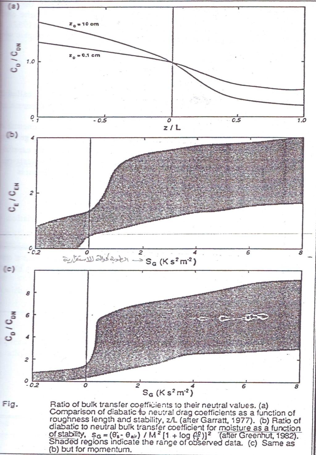
21 Q13) Knowing the shear ( dm ) at any height z is sufficient to determine the friction velocity ( u* ) for a neutral surface layer : dz u = k z dm dz If, however, you do not know the local shear, but instead know the value of the wind speed M 2 and M 1 at the heights z2 and z1 respectively, then you could use the following alternative expression to find u* : u*= k M Z*, derive the exact expression for Z*. z Q14 ) given the following wind speed data for a neutral surface layer, find the roughness length ( z0 ), the displacement distance ( d), and the friction velocity ( u* ) : Z ( m) M ( m/s ) Q15 ) a) given the following was observed over farmland on an overcast day : u* = 0.4 m/s, d=0, M = 5 m/s at z= 10m, find z0. b) suppose that the following was observed on a clear night ( No clouds ) over the same farmland : L= 30m, u*= 0.2m/s, find M at z= 1, 10 and 20 m. c) plot the wind speed profile from (a) and ( b) on semi-log graph paper. Q16) given the following data : w θ = 0.2 m s 0.4, z 0 = 0.01, z = 6m find : a) L ( the Obukhov length ) b) z/l, z i = 500m, g θ = m k, u s = 0.2 m, k = s Q17 ) the wind speed = 3m/s at a height of 4m. the ground surface has a roughness length of z0= 0.01m. find the value of u* for a) A convective daytime boundary layer where Ri = -0.5 b) A nocturnal boundary layer where Ri = 0.5. (21)