Mellor-Yamada Level 2.5 Turbulence Closure in RAMS. Nick Parazoo AT 730 April 26, 2006

Size: px

Start display at page:

Download "Mellor-Yamada Level 2.5 Turbulence Closure in RAMS. Nick Parazoo AT 730 April 26, 2006"

Rudolf Briggs
6 years ago
Views:

1 Mellor-Yamada Level 2.5 Turbulence Closure in RAMS Nick Parazoo AT 730 April 26, 2006

2 Overview Derive level 2.5 model from basic equations Review modifications of model for RAMS Assess sensitivity of vertical eddy diffusivities to tunable coefficients Feasibility of lookup table for RAMS

3 Goal of Mellor and Yamada Establish a hierarchy of turbulent closure models for planetary boundary layers by the following method 1. Obtain prognostic equations for the variance and covariance of the fluctuating components of velocity and potential temperature 2. Simplify higher level equations according to the number of isotropic components to retain, degree of computational efficiency 3. Introduce empirical constants that cover the most appropriate scales of turbulence

4 The Basic Equations Derive prognostic equations for Reynolds stress and heat conduction moments by combining equations for the mean and fluctuating components

5 Governing Equations To obtain closure, Mellor and Yamada use their own version of the Rotta- Kolmogorov model to approximate higher-moment terms

6 Governing Equations Energy redistribution hypothesis of Rotta (1951) Suggested could be made proportional to Reynolds stress and mean wind shear

7 Governing Equations Kolmogorov hypothesis of local, small-scale isotropy

8 Governing Equations 3rd order moment turbulent velocity diffusion terms are are scaled to 2nd order gradients

9 Governing Equations Some additional simplifications Coriolis force assumed negligible Hanjalic and Launder (1972) assume pressure diffusional terms are small Insert closure assumptions into the mean, turbulent momentum equations

10 Includes all terms in TKE evolution Used by Deardorff (1973) to model 3D and unsteady flows Since not very practical for most flows, can simplify by ordering terms as products of anisotropy parameter, a, which is assumed to be small, and q 3 /Λ The Level 4 Model

11 From Level 4 Assume diffusion and advection terms are equal and O(Uq 2 /L) Assume Uq 2 /L=aq 3 /Λ Neglect O(a 2 ) terms Neglects time-rate-ofchange, advection, and diffusion terms for anisotropic components of turbulence moments Level 3 retains prognostic equations only for TKE and <θ 2 > Level 3 Model

12 The Level 2.5 Model From Level 3, neglect material derivative and diffusion of potential temperature variance (22) Level 2.5 retains isotropic components of transient and diffusive turbulent processes Benefits of Level 3 scheme without computational cost Can simplify further by using BL approximation Make hydrostatic assumption Horizontal gradients small Horizontal divergence of turbulent fluxes ignored

13 Level 2.5 model Use 1.5 order closure and introduce dimensionless variables (Gh, Gm, Sh, Sm) to approximate flux terms in (20)-(23) Sq chosen as 0.2 Solving this system of equations is very straightforward

14 All length scales proportional to a single length scale and empirical constants Level 2.5 Model RAMS uses Blackadar s (1962) formula with ratio of TKE moments for l 0 and α=.10 as suggested by MY74 RAMS also assigns an upper limit for l in stable conditions according to André et al. (1978) so that scheme applies to full range of atmospheric forcing l = min(l,l D )

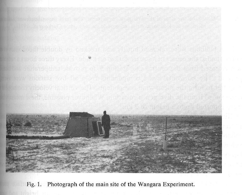
15 Level 2.5 Model Empirical constants based on neutral boundary layer and pipe data Tested/tuned model against neutral observations from day 33 of Wangara Experiment SE Australia, flat, uniform vegetation, little slope, short sparse grass (A 1, B 1, A 2, B 2,C 1 ) = (.92,16.6,0.74,10.1,0.08) for Mellor-Yamada 82 (A 1, B 1, A 2, B 2,C 1 ) = (.78,15.0,0.79,8.0,0.23) for Mellor 73

17 Level 2.5 Moisture Effects Brunt-Väisälä frequency chosen according to moisture levels (as recommended by MY82) g A θ e z q w z N 2 if moist saturated = g 1 θ θ z q v z q w z if unsaturated 1.61εLq 1+ v R where A = θ 1 d T, q 1 + εl2 q w = total water, q v =water vapor, and v C p R d T 2 θ e = θ 1+ εlq vs C p T, q vs =saturation vapor mixing ratio

18 Deficiency of Level 2.5 Designed for the case of near-local equilibrium Performs well for decaying turbulence but fails in growing turbulence because of exclusion of growth rate, advection, vertical diffusion and rapid terms in the balance equations for the second moments

19 Changes to Level 2.5 Level 2.5 has been adapted for case of growing turbulence according to Helfand and Labraga, 1988 (HF88) Isotropy assumption fails when anisotropic terms become too large to ignore and q 2 /q e2 <1 (growing convective PBL) HL88 recommend the following modification of the nondimensional eddy diffusivities S and velocity variance σ equilibrium values ( ) r are obtained from level 2 closure which assumes a balance between production and dissipation approximates rapid terms independently from original scheme in terms of known quantities (e) r = B l 2 u (S m ) r z + v z where (S h ) r, (S m ) r R f, R i 2 S h ( ) r N 2 S m = e / e r (S m ) r, S h = e / e r (S h ) r σ u 2 = e / e r (σ u 2 ) r, σ v 2 = e / e r (σ v 2 ) r, σ w 2 = e / e r (σ w 2 ) r

20 RAMSifications of HF88 Results in continuous but unsmooth transition from growing to decaying turbulence, but the solution is physically satisfying Produces realistic evolution of the PBL and outperforms several other realizability constraint techniques

21 Sensitivity of Model Eddy diffusivity is the most important output of the PBL scheme and depends on 8 tunable coefficients S e, a e, A 1, A 2, B 1, B 2, C 1, α Simple test of eddy diffusivity for momentum and heat using neutrally stable BL profile of TKE, potential temperature, and wind from 15 LST, day 33 of Wangara Experiment Assess sensitivity to α and to two sets of empirical constants derived by MY82 and M73 using the original level 2.5 scheme

22 Boundary Layer Data

23 Recommended Alpha (.1) Eddy diffusivity more spread apart for Mellor 73 values Heat flux slightly larger for MY82 values Eddy viscosity max is at the correct height but should decrease with height >500m Heat and momentum flux compare well to MY model Heat flux is correctly positive below H bl with max at correct height Momentum flux is correctly negative above 500m

24 Doubled Alpha (.2) Mixing coefficients blow up in both Shouldn t be larger than ~ 100m 2 s -1 Momentum and heat flux not as badly affected in MY73 case Spikes in heat flux related to spikes in eddy diffusivity

25 The response to α=.05 is good in that the model doesn t blow up, but the eddy diffusivities are less than half of their original values Conclusion: The amount of mixing in the model is fairly strongly dependent on a combination of mixing parameters Half Alpha (.05)

26 Level 2.5 in RAMS Compute vertical wind shear and N 2 separately and then feed into PBL subroutine Given TKE, wind shear, and N 2 for each grid point and vertical level, compute master length scale, nondimensional vertical gradients (G h, G m ), nondimensional eddy diffusivities (S h, S m ), and eddy diffusivities for heat and momentum for 2 scenarios: 1. tker > tkep (growing turbulence) 2. tker <= tkep (neutral/decaying turbulence) Excluding external variables, each case requires the calculation of about 10 dependent variables

27 Lookup Table Matsui et al (2004) notes that the computational burden of parameterizations can be reduced in two different ways 1. Reduce level of complexity of model 2. Pre-compute every possible output and store in a LUT Since there are only three inputs into the model and only a few equations to solve, it seems that the first approach been implicitly satisfied Plots of eddy diffusivity, however, leads me to believe that the range of possible outputs is fairly limited and a LUT could be at least mildly beneficial

28 Hybrid LUT Allow model to solve for master length scale (l) Call LUT after l is computed Input is l, tke, shear, and N 2 Output is the updated eddy diffusivity and TKE Use Similarity Theory and Buckingham Pi Theory to reduce inputs (as in Zinn et al, 1995) 4 variables (m): square of wind shear (sh = 1/S 2 ), Brunt-Vaisalla frequency (en2 = 1/S 2 ), mixing length (l = L), tke (e = L 2 /S 2 ) 2 dimensions (n): S and L Key variables (m-n=2): en2, e Dimensionless Pi groups: π 1 =en2/sh, π 2 =l*(sh/e) 1/2

29 Additional Steps: Hybrid LUT The next step would be to perform an experiment to determine values of the dimensionless groups Next, fit an empirical curve or regress an equation to data to describe relationship between groups Develop equations to relate eddy diffusivity and/or TKE to the dimensionless groups Create a lookup table from the equations and compare results to parameterization results and observations Level 3 output indicate that it might be possible to relate eddy diffusivity to π 1 and π 2

30 12 LST: neutral/stable, tke growing, little wind shear, l is small --> Km growing 3 LST: stable, tke~0, some wind shear, l is average --> Km~0

31 References Matsui, T., G. Leoncini, R.A. Pielke Sr., and U.S. Nair, 2004: A new paradigm for parameterization in atmospheric models: Application to the new Fu-Liou radiation code, Atmospheric Science Paper No. 747, Colorado State University, Fort Collins, CO 80523, 32 pp. Zinn, H.P., Kowalski, A.D., An efficient PBL Model For Global Circulation Models - Design and Validation, Boundary-Layer Meteorology, 75: 25-59, 1995

32 Shortcomings of Model Tuned against homogeneous neutral atmosphere and not designed for rapidly growing turbulence Turbulent length scale is not clearly defined Boundary layer height typically underestimated

1 Introduction to Governing Equations 2 1a Methodology... 2

Contents 1 Introduction to Governing Equations 2 1a Methodology............................ 2 2 Equation of State 2 2a Mean and Turbulent Parts...................... 3 2b Reynolds Averaging.........................