STATISTICS OF CLIMATE EXTREMES// TRENDS IN CLIMATE DATASETS

Transcription

1 STATISTICS OF CLIMATE EXTREMES// TRENDS IN CLIMATE DATASETS Richard L Smith Departments of STOR and Biostatistics, University of North Carolina at Chapel Hill and Statistical and Applied Mathematical Sciences Institute (SAMSI) SAMSI Graduate Class November 14,

2 EXAMINE SST AS AN ALTERNATIVE COVARIATE Define Gulf Coast Region and 80 neighboring precipitation stations (Houston Hobby in black) Calculate monthly mean SST for Gulf Coast Region 2

3 3

4 ESTIMATES FOR HOUSTON HOBBY AIRPORT 4

5 1. Use 7-day annual maximum precipitation (also tried 3, 4, 5, 6, 8 days: similar results) 2. Fit linear trend in GEV location parameter: p Examine all possible consecutive sequences of monthly SST lags from 0 12 months (91 possible covariates) 4. Best SST model uses means of lags 7, 8, 9, p , but this raises an obvious selection bias issue 5. I could not come up with any argument why the SST analysis was better than the linear trend analysis after taking account of the selection bias issue 6. Therefore, try a combined analysis over many stations 5

6 Here is a table of the 10 best models ordered by the deviance-based P-value, with the SST lags that are included in each. Lags P-value 7,8, , ,8,9, ,6,7,8,9, ,7,8,9, ,7,8, ,6,7,8, ,5,6,7,8,9, ,4,5,6,7,8,9, Conclusion: Lags 6 10 all feature in many models Difficult to quantify the effect of selection bias Benjamini-Hochberg test for the False Discovery Rate not valid because the tests are not independent Even so, 10 P-values that are less than (out of 91 models tested) seems to be unlikely to occur by chance 6

7 COMBINED ESTIMATES FOR 80 GULF COAST STATIONS 7

8 1. Initial analysis not promising: many stations showed no statisticially significant trend 2. Definition of SST variable: Settled on averages of lags 7 12 months 3. Based on 7-day maxima, 16 (out of 80) have a statistically significant linear trend at p = 0.05, 13 have a statistically significant SST trend at p = Must be wary of selection bias issues, but these are still greater numbers than could be explained just by chance 5. Therefore, proceed to a full spatial analysis 8

9 Spatial Analysis (Similar to: D.M. Holland, V. De Oliveira, L.H. Cox and R.L. Smith (2000), Estimation of regional trends in sulfur dioxide over the eastern United States. Environmetrics 11, ) Let Z be full spatial field of the linear trend (Z(s) is true trend at location s). Let Ẑ be estimated spatial field at stations s 1,..., s n. Model: Ẑ Z N (Z, W), Z N (0, V(θ)) where W is assumed known and V(θ) is the covariance matrix of some spatial field I use exponential covariance matrix where θ is range. So Ẑ N (0, W + V(θ)) and Z may be reconstructed from Ẑ by kriging (Estimation of W uses bootstrapping) 9

10 I estimated this model using 1. Ẑ is vector of linear trend estimates at each station 2. Ẑ is vector of SST trend estimates at each station 3. Also considered adjusted analysis: put in both linear trend and residuals from SSTs regressed on linear trend (two covariates in same model, kriging done separately for each) 10

11 RESULTS 11

12 Estimates of Overall Trend Parameter Model Estimate Standard Error t Statistics P-value SST alone SST adjusted Linear alone Linear adjusted

13 Image Plot Based on SST Trends latpred lonpred 13

14 Image Plot Based on Adjusted SST Trends latpred lonpred 14

15 Image Plot Based on Linear Trends latpred lonpred 15

16 Image Plot Based on Adjusted Linear Trends latpred lonpred 16

17 Noboot option Instead of using the bootstrap to estimate the matrix W, we simply assumed W was diagonal, with diagonal entries corresponding to the squares of the standard errors in the GEV fitting procedure (in other words: estimates are independent from station to station) The spatial model fitting procedure was repeated, and the new images plotted. The results were very little different. 17

18 Estimates of Overall Trend Parameter Model Estimate Standard Error t Statistics P-value SST alone SST adjusted Linear alone Linear adjusted

19 Image Plot Based on SST Trends (noboot) latpred lonpred 19

20 Image Plot Based on Adjusted SST Trends (noboot) latpred lonpred 20

21 Image Plot Based on Linear Trends (noboot) latpred lonpred 21

22 Image Plot Based on Adjusted Linear Trends (noboot) latpred lonpred 22

23 To do: 1. Rerun the bootstrap procedure to correct for a possible error in constructing the bootstrap samples (discussed during the talk) 2. Interpolate α, σ, ξ in same way and hence construct estimates of threshold exceedance probabilities at different locations under the spatially interpolated model 3. Remark: Direct interpolation of threshold probabilities from site to site doesn t work; estimates are too variable for the spatial model to fit 23

24 CONCLUSIONS 1. Adjusted model shows a clear separation in contributions of the linear and SST components 2. SST component seems particularly concentrated on Houston, whether adjusted or not 3. Linear trend shows a less definitive pattern 4. Future work: (a) Draw similar plots for estimated probabilities of a Harveylevel exceedance (b) Compare extreme value probabilities for different dates (e.g v. 1950) (c) Integrate with CMIP5 model projections for future extreme probabilities (d) POT alternative analysis? 24

25 TIME SERIES ANALYSIS FOR CLIMATE DATA I Overview II The post-1998 hiatus in temperature trends III NOAA s record streak IV Trends or nonstationarity? 25

26 TIME SERIES ANALYSIS FOR CLIMATE DATA I Overview II The post-1998 hiatus in temperature trends III NOAA s record streak IV Trends or nonstationarity? 26

27 HadCRUT4 gl Global Temperatures Global Temperature Anomaly Slope 0.74 degrees/century OLS Standard error Year 27

28 What s wrong with that picture? We fitted a linear trend to data which are obviously autocorrelated OLS estimate 0.74 deg C per century, standard error So it looks statistically significant, but question how standard error is affected by the autocorrelation First and simplest correction to this: assume an AR(1) time series model for the residual So I calculated the residuals from the linear trend and fitted an AR(1) model, X n = φ 1 X n 1 + ɛ n, estimated ˆφ 1 = 0.62 with standard error With this model, the standard error of the OLS linear trend becomes 0.057, still making the trend very highly significant But is this an adequate model? 28

29 ACF of Residuals from Linear Trend ACF Sample ACF AR(1) Lag 29

30 Fit AR(p) of various orders p, calculate log likelihood, AIC, and the standard error of the linear trend. Model X n = p i=1 φ ix n i + ɛ n, ɛ n N[0, σ 2 ɛ ] (IID) AR order LogLik AIC Trend SE

31 Extend the calculation to ARMA(p,q) for various p and q: model is X n p i=1 φ ix n i = ɛ n + q j=1 θ jɛ n j, ɛ n N[0, σɛ 2 ] (IID) AR order MA order SE of trend based on ARMA(1,4) model: deg C per century 31

32 ACF of Residuals from Linear Trend ACF Sample ACF AR(6) ARMA(1,4) Lag 32

33 Calculating the standard error of the trend Estimate ˆβ = n i=1 w i X i, variance σɛ 2 n n i=1 j=1 w i w j ρ i j where ρ is the autocorrelation function of the fitted ARMA model Alternative formula (Bloomfield and Nychka, 1992) Variance(ˆβ) = 2 1/2 0 w(f)s(f)df where s(f) is the spectral density of the autocovariance function and w(f) = is the transfer function n j=1 w n e 2πijf 2 33

34 Example based on Barnes and Barnes (Journal of Climate, 2015) They compared the OLS estimator of a linear regression with the epoch estimator computed by taking the difference between the first M and last M values of a series of length N, for some M < N 2. The epoch estimator is then rescaled so that it is in the same units as the classical linear regression estimator. Question: Which performs better under various time series assumptions on the underlying series? The following plot shows the transfer functions for N = 100, M = 33, epoch estimator in red, OLS in blue. Generally the OLS estimator is better, but not if the series has a spectral peak near

35 Transfer Function Times Ratio of Mean Red and Blue Curves is Frequency 35

36 What s better than the OLS linear trend estimator? Use generalized least squares (GLS) y n = β 0 + β 1 x n + u n, u n ARMA(p, q) Repeat same process with AIC: ARMA(1,4) again best ˆβ = 0.73, standard error

37 Calculations in R ip=4 iq=1 ts1=arima(y2,order=c(ip,0,iq),xreg=1:ny,method= ML ) Coefficients: ar1 ar2 ar3 ar4 ma1 intercept 1:ny s.e sigma^2 estimated as : log likelihood = 106.8, aic = acf1=armaacf(ar=ts1$coef[1:ip],ma=ts1$coef[ip+1:iq],lag.max=150) 37

38 TIME SERIES ANALYSIS FOR CLIMATE DATA I Overview II The post-1998 hiatus in temperature trends III NOAA s record streak IV Trends or nonstationarity? 38

39 HadCRUT4 gl Temperature Anomalies Global Temperature Anomaly Year 39

40 HadCRUT4 gl Temperature Anomalies Global Temperature Anomaly Year 40

41 NOAA Temperature Anomalies Global Temperature Anomaly Year 41

42 NOAA Temperature Anomalies Global Temperature Anomaly Year 42

43 GISS (NASA) Temperature Anomalies Global Temperature Anomaly Year 43

44 GISS (NASA) Temperature Anomalies Global Temperature Anomaly Year 44

45 Berkeley Earth Temperature Anomalies Global Temperature Anomaly Year 45

46 Berkeley Earth Temperature Anomalies Global Temperature Anomaly Year 46

47 Cowtan Way Temperature Anomalies Global Temperature Anomaly Year 47

48 Cowtan Way Temperature Anomalies Global Temperature Anomaly Year 48

49 Statistical Models Let t 1i : ith year of series y i : temperature anomaly in year t i t 2i = (t 1i 1998) + y i = β 0 + β 1 t 1i + β 2 t 2i + u i Simple linear regression (OLS): u i N[0, σ 2 ] (IID) Time series regression (GLS): u i φ 1 u i 1... φ p u i p = ɛ i + θ 1 ɛ i θ q ɛ i q, ɛ i N[0, σ 2 ] (IID) Fit using arima function in R 49

50 HadCRUT4 gl Temperature Anomalies OLS Fit, Changepoint at 1998 Global Temperature Anomaly Change of slope 0.85 deg/cen (SE 0.50 deg/cen) Year 50

51 HadCRUT4 gl Temperature Anomalies GLS Fit, Changepoint at 1998 Global Temperature Anomaly Change of slope 1.16 deg/cen (SE 0.4 deg/cen) Year 51

52 NOAA Temperature Anomalies GLS Fit, Changepoint at 1998 Global Temperature Anomaly Change of slope 0.21 deg/cen (SE 0.62 deg/cen) Year 52

53 GISS (NASA) Temperature Anomalies GLS Fit, Changepoint at 1998 Global Temperature Anomaly Change of slope 0.29 deg/cen (SE 0.54 deg/cen) Year 53

54 Berkeley Earth Temperature Anomalies GLS Fit, Changepoint at 1998 Global Temperature Anomaly Change of slope 0.74 deg/cen (SE 0.6 deg/cen) Year 54

55 Cowtan Way Temperature Anomalies GLS Fit, Changepoint at 1998 Global Temperature Anomaly Change of slope 0.93 deg/cen (SE 1.24 deg/cen) Year 55

56 Adjustment for the El Niño Effect El Niño is a weather effect caused by circulation changes in the Pacific Ocean 1998 was one of the strongest El Niño years in history A common measure of El Niño is the Southern Oscillation Index (SOI), computed monthly Here use SOI with a seven-month lag as an additional covariate in the analysis 56

57 HadCRUT4 gl With SOI Signal Removed GLS Fit, Changepoint at 1998 Global Temperature Anomaly Change of slope 0.81 deg/cen (SE 0.75 deg/cen) Year 57

58 NOAA With SOI Signal Removed GLS Fit, Changepoint at 1998 Global Temperature Anomaly Change of slope 0.18 deg/cen (SE 0.61 deg/cen) Year 58

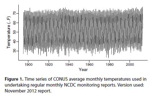
59 GISS (NASA) With SOI Signal Removed GLS Fit, Changepoint at 1998 Global Temperature Anomaly Change of slope 0.24 deg/cen (SE 0.54 deg/cen) Year 59

60 Berkeley Earth With SOI Signal Removed GLS Fit, Changepoint at 1998 Global Temperature Anomaly Change of slope 0.69 deg/cen (SE 0.58 deg/cen) Year 60

61 Cowtan Way With SOI Signal Removed GLS Fit, Changepoint at 1998 Global Temperature Anomaly Change of slope 0.99 deg/cen (SE 0.79 deg/cen) Year 61

62 Selecting The Changepoint If we were to select the changepoint through some form of automated statistical changepoint analysis, where would we put it? 62

63 HadCRUT4 gl Change Point Posterior Probability Posterior Probability of Changepoint Year 63

64 Conclusion from Temperature Trend Analysis No evidence of decrease post-1998 if anything, the trend increases after this time After adjusting for El Niño, even stronger evidence for a continuously increasing trend If we were to select the changepoint instead of fixing it at 1998, we would choose some year in the 1970s Thus: No statistical evidence to support the hiatus hypothesis 64

65 TIME SERIES ANALYSIS FOR CLIMATE DATA I Overview II The post-1998 hiatus in temperature trends III NOAA s record streak IV Trends or nonstationarity? 65

66 66

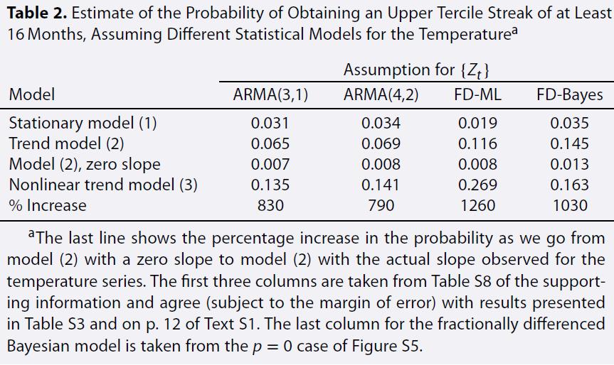
67 Continental US monthly temperatures, Jan 1895 Oct For each month between June 2011 and Sep 2012, the monthly temperature was in the top tercile of all observations for that month up to that point in the time series. Attention was first drawn to this in June 2012, at which point the series of top tercile events was 13 months long, leading to a naïve calculation that the probability of that event was (1/3) 13 = Eventually, the streak extended to 16 months, but ended at that point, as the temperature for Oct 2012 was not in the top tercile. In this study, we estimate the probability of either a 13-month or a 16-month streak of top-tercile events, under various assumptions about the monthly temperature time series. 67

68 68

69 69

70 70

71 71

72 Method Two issues with NOAA analysis: Neglects autocorrelation Ignores selection effect Solutions: Fit time series model ARMA or long-range dependence Use simulation to determine the probability distribution of the longest streak in 117 years Some of the issues: Selection of ARMA model AR(1) performs poorly Variances differ by month must take that into account Choices of estimation methods, e.g. MLE or Bayesian Bayesian methods allow one to take account of parameter estimation uncertainty 72

73 73

74 74

75 Conclusions It s important to take account of monthly varying standard deviations as well as means. Estimation under a high-order ARMA model or fractional differencing lead to very similar results, but don t use AR(1). In a model with no trend, the probability that there is a sequence of length 16 consecutive top-tercile observations somewhere after year 30 in the 117-year time series is of the order of , depending on the exact model being fitted. With a linear trend, these probability rise to something over.05. Include a nonlinear trend, and the probabilities are even higher in other words, not surprising at all. Overall, the results may be taken as supporting the overall anthropogenic influence on temperature, but not to a stronger extent than other methods of analysis. 75

76 TIME SERIES ANALYSIS FOR CLIMATE DATA I Overview II The post-1998 hiatus in temperature trends III NOAA s record streak IV Trends or nonstationarity? 76

77 A Parliamentary Question is a device where any member of the U.K. Parliament can ask a question of the Government on any topic, and is entitled to expect a full answer. 77

78 April 22,

79 79

80 Essence of the Met Office Response Acknowledged that under certain circumstances an ARIMA(3,1,0) without drift can fit the data better than an AR(1) model with drift, as measured by likelihood The result depends on the start and finish date of the series Provides various reasons why this should not be interpreted as an argument against climate change Still, it didn t seem to me (RLS) to settle the issue beyond doubt 80

81 There is a tradition of this kind of research going back some time 81

82 82

83 Summary So Far Integrated or unit root models (e.g. ARIMA(p, d, q) with d = 1) have been proposed for climate models and there is some statistical support for them If these models are accepted, the evidence for a linear trend is not clear-cut Note that we are not talking about fractionally integrated models (0 < d < 2 1 ) for which there is by now a substantial tradition. These models have slowly decaying autocorrelations but are still stationary Integrated models are not physically realistic but this has not stopped people advocating them I see the need for a more definitive statistical rebuttal 83

84 HadCRUT4 Global Series, Model I : y t y t 1 = ARMA(p, q) (mean 0) Model II : y t = Linear Trend + ARMA(p, q) Model III : y t y t 1 = Nonlinear Trend + ARMA(p, q) Model IV : y t = Nonlinear Trend + ARMA(p, q) Use AICC as measure of fit 84

85 Integrated Time Series, No Trend p q NA

86 Stationary Time Series, Linear Trend p q NA

87 Integrated Time Series, Nonlinear Trend p q NA

88 Stationary Time Series, Nonlinear Trend p q NA

89 Integrated Mean 0 Stationary Linear Trend Series Series Year Year Integrated Nonlinear Trend Stationary Nonlinear Trend Series Series Year Year Four Time Series Models with Fitted Trends 89

90 Integrated Mean 0 Stationary Linear Trend Residual Residual Year Year Integrated Nonlinear Trend Stationary Nonlinear Trend Residual Residual Year Year Residuals From Four Time Series Models 90

91 Integrated Mean 0 Stationary Linear Trend Residual Residual Year Year Integrated Nonlinear Trend Stationary Nonlinear Trend Residual Residual Year Year Residuals From Four Time Series Models 91

92 Conclusions If we restrict ourselves to linear trends, there is not a clearcut preference between integrated time series models without a trend and stationary models with a trend However, if we extend the analysis to include nonlinear trends, there is a very clear preference that the residuals are stationary, not integrated Possible extensions: Add fractionally integrated models to the comparison Bring in additional covariates, e.g. circulation indices and external forcing factors Consider using a nonlinear trend derived from a climate model. That would make clear the connection with detection and attribution methods which are the preferred tool for attributing climate change used by climatologists. 92