FIN822 project 2 Project 2 contains part I and part II. (Due on November 10, 2008)

Transcription

1 FIN822 project 2 Project 2 contains part I and part II. (Due on November 10, 2008) Part I Logit Model in Bankruptcy Prediction You do not believe in Altman and you decide to estimate the bankruptcy prediction model using the following logit model: y= Λ (a+b1* X1+b2* X2+b3* X3+b4* X4+b5* X5) + error term where variables are defined as: X1: re_ta=retainedearnings/totalassets X2: cacl_ta=(totalcurrentassetstotalcurrentliabilities)/totalassets X3: ebit_ta=earningsbeforeinterestandtaxes/totalassets (Do not use ROA) X4: totalliabilities/totalassets X5: totalrevenue/totalassets y= banc_indicator: a dummy variable that takes value of 1 if the firm goes bankrupt in year 2004 or 2005, and 0 otherwise. Download data that I have constructed from my web Say a few words on your sample (how many firms in total, how many went bankruptcy? etc). Report your estimated coefficients and the respective t-statistics (or p-values). Which variable(s) are significant at 0.05 levels? Do the results make sense? Based on your logit model output, what is the estimated bankruptcy probability for a firm with the following ratios: x1=0.2, x2=1, x3= - 20%, x4=0.7, x5=1? (Think of the in-class-work question on high school student graduation probability.) Tips: For illustration I will used an abbreviated version of the dataset which contains fewer observations. You should use the full sample.

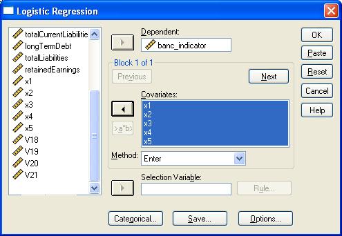
2 Analyze>Regression>Binary Logistic 2

3 Coefficients are given in this table (you should expect different results): B are estimated coefficients, Sig. are the p-values. Ignore other statistics. Step 1 a x1 x2 x3 x4 x5 Variables in the Equation B S.E. Wald df Sig. Exp(B) Constant a. Variable(s) entered on step 1: x1, x2, x3, x4, x5. The numbers of non-bankrupt and bankrupt firms can be seen from this table: Classification Table(a,b) Predicted Percentage banc_indicator Correct Observed Step banc_indicator Overall Percentage 99.3 a Constant is included in the model. b The cut value is.500 3

4 Part II. Conduct an analysis on a time series. Download data that I have constructed from Explain how you have chosen the number of lags (p=?, q=?) in your ARIMA model. Write down the dynamic structure for the original time series. A tutorial is attached below. You can estimate the time series using either of the two approaches illustrated in the example below. Time-Series Analysis Example Suppose you are given a time-series. The example data is available from my website at First, load in SPSS. If you see the following window, click cancel. Then open the excel file. Note that you should choose All Files (*.*) in the following window. Otherwise you may not see the excel file. 4

5 Click Ok if you see this. 5

6 Let s take a look at the time-series plot. Pull down the menu: Analyze> Times Series> Sequence Chart Then choose Y and X axis, and click OK Copy object and paste it below. The plot looks like this x

7 If you want to see a better-looking picture with horizontal axis shown, you have to export the graph as a PDF file or PowerPoint file and then select-paste it. What a pain It will look like this. Clearly there is a trend in this series. So I can either (1) run a regression on time (t) and get the residuals, or (2) compute the first difference. 7

8 First approach: regress the series on t Analyze>regression>linear Choose X as dependent variable, t as independent variable. Also click Save 8

9 Select Unstandarized Residuals in the above window. This will save the residual from regression. Click Continue, OK Here is regression output: Coefficients(a) Unstandardized Coefficients Standardized Coefficients t Sig. Model B Std. Error Beta B Std. Error 1 (Constant) t a Dependent Variable: x You also see estimated residuals in the 3 rd column in the SPSS data window. (Below) 9

10 Now let s see a plot of the residual. It appears stationary Unstandardized Residual

11 Then let s draw the autocorrelation function (ACF) and partial-autocorrelation function (PACF) graphs for this residual. Analyze>Times Series>Autocorrelations Choose the unstandarized residuals as our interested variables. Click OK. Unstandardized Residual 1.0 Coefficient Upper Confidence L Lower Confidence L 0.5 ACF

12 Unstandardized Residual 1.0 Coefficient Upper Confidence L Lower Confidence L 0.5 Partial ACF From the above graphs, the ACF decays gradually while the PACF stands out only for lag 1. So a ARIMA(1,0,0)=ARMA(1,0)=AR(1) model may be appropriate. You also see some info like this 12

13 Series: Unstandardized Residual Lag Autocorrelations Autocorrel Box-Ljung Statistic ation Std. Error a Value df Sig. b a. The underlying process assumed is independence (white noise). b. Based on the asymptotic chi-square approximation. The p-value (Sig.) based on Box-Ljung statistic is significant for each lag. This means the time-series of unstandarized residuals are significantly different from a white noise process by examining all autocorrelations up to that lag. (We already know this because, from the two graphs above, the ACF and PACF at lag 1 are significant.) Then run the ARIMA model, Analyze>Times Series> ARIMA 13

14 Choose 1 for p and click OK. Choose Unstandarized residuals as the variable Then you will see this. It tells us that SPSS will add some residuals, fitted variable, and confidence intervals, to our dataset. Click OK. Here is the ARIMA coefficient estimate: Parameter Estimates Estimates Std Error t Approx Sig Non-Seasonal Lags AR Constant Melard's algorithm was used for estimation. (About the constant term: When d=0 a constant term equals to the mean of the time series. When d=1 a constant term reflects the non-zero average trend of the original time series.) 14

15 In the data window we also see that the residual from ARIMA modeling, under the name ERR_1 Did our model do a good job? Let s see the ACF and PACF of the new residual ERR_1 (This is the residual from ARIMA model, not the one from linear regression) Analyze>Times Series> Autocorrelations... Then update the name of our interested variable (as shown in the window below 15

16 Click OK. Error for RES_1 from ARIMA, MOD_2, CON 1.0 Coefficient Upper Confidence L Lower Confidence L 0.5 ACF Error for RES_1 from ARIMA, MOD_2, CON 1.0 Coefficient Upper Confidence L Lower Confidence L 0.5 Partial ACF No significant ACF or PACF, so the residual from our ARIMA modeling seems to be white noise. Our modeling job has finished. 16

17 What is the structure of the original time series? Let me call the residual from the linear regression (first step) z. So from ARIMA modeling: Parameter Estimates Estimates Std Error t Approx Sig Non-Seasonal Lags AR Constant Melard's algorithm was used for estimation. (About the constant term: When d=0 a constant term equals to the mean of the time series. When d=1 a constant term reflects the non-zero average trend of the original time series.) We have: ( z 0.011) = 0.451*( z 0.011) + ε (1) t t 1 t From step 1 linear regression, we know that x = * t+ z (2) t t Combing the two equations (1) and (2) together, we have ( x * t 0.011) = 0.451*( x *( t 1) 0.011) + ε t t 1 t That can be simplified as: x = * x * t+ ε (3) t t 1 t (3) is our description of the original time-series. 17

18 Second approach: Using the first difference Open the excel data file, compute first difference and call the variable u. Save the file. In SPSS, open the excel file just saved. Files of Type should choose All Files (*.*) Click OK 18

19 Plot the differenced series u. Analyze>Times Series>Sequence chart It appears stationary u Then plot the ACF and PACF graph for u ( u is the first difference of the original series ) 19

20 u 1.0 Coefficient Upper Confidence L Lower Confidence L 0.5 ACF u 1.0 Coefficient Upper Confidence L Lower Confidence L 0.5 Partial ACF The ACF and PACF both seems to decay over lags. So I choose an ARMA(1,1) model. (Some people might think it is an MA(1) but you will find out the residual from an MA(1) does not really follow a white noise. Sometimes the estimation does require try-and-error. ) 20

21 To estimate the parameters, we go Analyze > Times Series > ARIMA Select the differenced series u as dependent variable.then choose p=1 and q=1 in the window below. Alternatively, you can specify: p=1, d=1, and q=1 for the original series x. You will get same output. 21

22 Click Ok Click Ok Below is our model parameter estimates Parameter Estimates Estimates Std Error t Approx Sig Non-Seasonal AR Lags MA Constant Melard's algorithm was used for estimation. (About the constant term: When d=0 a constant term equals to the mean of the time series. When d=1 a constant term reflects the non-zero average trend of the original time series.) Did the model do a good job? We can check the ACF, PACF of the newly obtained residual and the Box- Ljung statistics. 22

23 Error for u from ARIMA, MOD_1, CON Error for u from ARIMA, MOD_1, CON 1.0 Coefficient Upper Confidence L Lower Confidence L 1.0 Coefficient Upper Confidence L Lower Confidence L ACF 0.0 Partial ACF Judging from the ACF and PACF the residual from ARIMA seems to be white noise, also the Box-Ljung statistics are not significant, so we can stop now. Autocorrelations Series: Error for u from ARIMA, MOD_1, CON Lag Autocorrel Box-Ljung Statistic ation Std. Error a Value df Sig. b a. The underlying process assumed is independence (white noise). b. Based on the asymptotic chi-square approximation. 23

24 What is the structure of the original time series? From ARIMA modeling, we have Parameter Estimates Estimates Std Error t Approx Sig Non-Seasonal AR Lags MA Constant Melard's algorithm was used for estimation. (About the constant term: When d=0 a constant term equals to the mean of the time series. When d=1 a constant term reflects the non-zero average trend of the original time series.) So, ( u 0.794) = 0.470( u 0.794) + ε 0.986* ε (4) t t 1 t t 1 By the way, SPSS tries to behave special and naughty, so unlike the general assumption as in other softwares which assume: X = φ X + φ X φ X + ε + θε + θ ε θ ε SPSS would assume a form: X = φ X + φ X φ X + ε θε θ ε... θ ε That is why you see a negative for the coefficient before In step 1, we took a first difference. That means: Combining the (4) and (5), we get: t 1 t 1 2 t 2 p t p t 1 t 1 2 t 2 q t q t 1 t 1 2 t 2 p t p t 1 t 1 2 t 2 q t q εt 1 xt = xt 1 + ut (5) x = x 0.47x + ε ε (6) t t 1 t 2 t t 1 (6) is our description of the original time-series. 24

25 Final comments Using two approaches we have derived the structure (3) and (6) respectively for the original time series. Are the structure (3) and (6) similar? (Did we get similar results using two different approaches?) Below I will show you that the two results indeed are very close. x = x * t+ ε (3) t t 1 t From (3) we can write xt 1 as x = x ( t 1) + ε (3') t 1 t 2 t 1 Subtract (3 ) from (3), we get x x = 0.451x 0.451x ε ε t t 1 t 1 t 2 t t 1 Which can be simplified to x = x 0.451x + ε ε t t 1 t 2 t t 1 This indeed is very close to equation (6) we derived using the second approach. 25