STATISTICS FOR CLIMATE SCIENCE

Transcription

1 STATISTICS FOR CLIMATE SCIENCE Richard L Smith University of North Carolina and SAMSI VI-MSS Workshop on Environmental Statistics Kolkata, March 2-4,

2 In Memoriam Gopinath Kallianpur

3 I. TIME SERIES ANALYSIS FOR CLIMATE DATA I.a Overview I.b The post-1998 hiatus in temperature trends I.c NOAA s record streak I.d Trends or nonstationarity? II. CLIMATE EXTREMES II.a Extreme value models II.b An example based on track records II.c Applying extreme value models to weather extremes II.d Joint distributions of two of more variables II.e Conclusions, other models, future research 3

4 I. TIME SERIES ANALYSIS FOR CLIMATE DATA I.a Overview I.b The post-1998 hiatus in temperature trends I.c NOAA s record streak I.d Trends or nonstationarity? II. CLIMATE EXTREMES II.a Extreme value models II.b An example based on track records II.c Applying extreme value models to weather extremes II.d Joint distributions of two of more variables II.e Conclusions, other models, future research 4

5 HadCRUT4 gl Global Temperatures Global Temperature Anomaly Slope 0.74 degrees/century OLS Standard error Year 5

6 What s wrong with that picture? We fitted a linear trend to data which are obviously autocorrelated OLS estimate 0.74 deg C per century, standard error So it looks statistically significant, but question how standard error is affected by the autocorrelation First and simplest correction to this: assume an AR(1) time series model for the residual So I calculated the residuals from the linear trend and fitted an AR(1) model, X n = φ 1 X n 1 + ɛ n, estimated ˆφ 1 = 0.62 with standard error With this model, the standard error of the OLS linear trend becomes 0.057, still making the trend very highly significant But is this an adequate model? 6

7 ACF of Residuals from Linear Trend ACF Sample ACF AR(1) Lag 7

8 Fit AR(p) of various orders p, calculate log likelihood, AIC, and the standard error of the linear trend. Model X n = p i=1 φ ix n i + ɛ n, ɛ n N[0, σ 2 ɛ ] (IID) AR order LogLik AIC Trend SE

9 Extend the calculation to ARMA(p,q) for various p and q: model is X n p i=1 φ ix n i = ɛ n + q j=1 θ jɛ n j, ɛ n N[0, σɛ 2 ] (IID) AR order MA order SE of trend based on ARMA(1,4) model: deg C per century 9

10 ACF of Residuals from Linear Trend ACF Sample ACF AR(6) ARMA(1,4) Lag 10

11 Calculating the standard error of the trend Estimate ˆβ = n i=1 w i X i, variance σɛ 2 n n i=1 j=1 w i w j ρ i j where ρ is the autocorrelation function of the fitted ARMA model Alternative formula (Bloomfield and Nychka, 1992) Variance(ˆβ) = 2 1/2 0 w(f)s(f)df where s(f) is the spectral density of the autocovariance function and w(f) = is the transfer function n j=1 w n e 2πijf 2 11

12 12

13 What s better than the OLS linear trend estimator? Use generalized least squares (GLS) y n = β 0 + β 1 x n + u n, u n ARMA(p, q) Repeat same process with AIC: ARMA(1,4) again best ˆβ = 0.73, standard error

14 Calculations in R ip=4 iq=1 ts1=arima(y2,order=c(ip,0,iq),xreg=1:ny,method= ML ) Coefficients: ar1 ar2 ar3 ar4 ma1 intercept 1:ny s.e sigma^2 estimated as : log likelihood = 106.8, aic = acf1=armaacf(ar=ts1$coef[1:ip],ma=ts1$coef[ip+1:iq],lag.max=150) 14

15 I. TIME SERIES ANALYSIS FOR CLIMATE DATA I.a Overview I.b The post-1998 hiatus in temperature trends I.c NOAA s record streak I.d Trends or nonstationarity? II. CLIMATE EXTREMES II.a Extreme value models II.b An example based on track records II.c Applying extreme value models to weather extremes II.d Joint distributions of two of more variables II.e Conclusions, other models, future research 15

16 HadCRUT4 gl Temperature Anomalies Global Temperature Anomaly Year 16

17 HadCRUT4 gl Temperature Anomalies Global Temperature Anomaly Year 17

18 NOAA Temperature Anomalies Global Temperature Anomaly Year 18

19 NOAA Temperature Anomalies Global Temperature Anomaly Year 19

20 GISS (NASA) Temperature Anomalies Global Temperature Anomaly Year 20

21 GISS (NASA) Temperature Anomalies Global Temperature Anomaly Year 21

22 Berkeley Earth Temperature Anomalies Global Temperature Anomaly Year 22

23 Berkeley Earth Temperature Anomalies Global Temperature Anomaly Year 23

24 Cowtan Way Temperature Anomalies Global Temperature Anomaly Year 24

25 Cowtan Way Temperature Anomalies Global Temperature Anomaly Year 25

26 Statistical Models Let t 1i : ith year of series y i : temperature anomaly in year t i t 2i = (t 1i 1998) + y i = β 0 + β 1 t 1i + β 2 t 2i + u i Simple linear regression (OLS): u i N[0, σ 2 ] (IID) Time series regression (GLS): u i φ 1 u i 1... φ p u i p = ɛ i + θ 1 ɛ i θ q ɛ i q, ɛ i N[0, σ 2 ] (IID) Fit using arima function in R 26

27 HadCRUT4 gl Temperature Anomalies OLS Fit, Changepoint at 1998 Global Temperature Anomaly Change of slope 0.85 deg/cen (SE 0.50 deg/cen) Year 27

28 HadCRUT4 gl Temperature Anomalies GLS Fit, Changepoint at 1998 Global Temperature Anomaly Change of slope 1.16 deg/cen (SE 0.4 deg/cen) Year 28

29 NOAA Temperature Anomalies GLS Fit, Changepoint at 1998 Global Temperature Anomaly Change of slope 0.21 deg/cen (SE 0.62 deg/cen) Year 29

30 GISS (NASA) Temperature Anomalies GLS Fit, Changepoint at 1998 Global Temperature Anomaly Change of slope 0.29 deg/cen (SE 0.54 deg/cen) Year 30

31 Berkeley Earth Temperature Anomalies GLS Fit, Changepoint at 1998 Global Temperature Anomaly Change of slope 0.74 deg/cen (SE 0.6 deg/cen) Year 31

32 Cowtan Way Temperature Anomalies GLS Fit, Changepoint at 1998 Global Temperature Anomaly Change of slope 0.93 deg/cen (SE 1.24 deg/cen) Year 32

33 Adjustment for the El Niño Effect El Niño is a weather effect caused by circulation changes in the Pacific Ocean 1998 was one of the strongest El Niño years in history A common measure of El Niño is the Southern Oscillation Index (SOI), computed monthly Here use SOI with a seven-month lag as an additional covariate in the analysis 33

34 HadCRUT4 gl With SOI Signal Removed GLS Fit, Changepoint at 1998 Global Temperature Anomaly Change of slope 0.81 deg/cen (SE 0.75 deg/cen) Year 34

35 NOAA With SOI Signal Removed GLS Fit, Changepoint at 1998 Global Temperature Anomaly Change of slope 0.18 deg/cen (SE 0.61 deg/cen) Year 35

36 GISS (NASA) With SOI Signal Removed GLS Fit, Changepoint at 1998 Global Temperature Anomaly Change of slope 0.24 deg/cen (SE 0.54 deg/cen) Year 36

37 Berkeley Earth With SOI Signal Removed GLS Fit, Changepoint at 1998 Global Temperature Anomaly Change of slope 0.69 deg/cen (SE 0.58 deg/cen) Year 37

38 Cowtan Way With SOI Signal Removed GLS Fit, Changepoint at 1998 Global Temperature Anomaly Change of slope 0.99 deg/cen (SE 0.79 deg/cen) Year 38

39 Selecting The Changepoint If we were to select the changepoint through some form of automated statistical changepoint analysis, where would we put it? 39

40 HadCRUT4 gl Change Point Posterior Probability Posterior Probability of Changepoint Year 40

41 Conclusion from Temperature Trend Analysis No evidence of decrease post-1998 if anything, the trend increases after this time After adjusting for El Niño, even stronger evidence for a continuously increasing trend If we were to select the changepoint instead of fixing it at 1998, we would choose some year in the 1970s 41

42 I. TIME SERIES ANALYSIS FOR CLIMATE DATA I.a Overview I.b The post-1998 hiatus in temperature trends I.c NOAA s record streak I.d Trends or nonstationarity? II. CLIMATE EXTREMES II.a Extreme value models II.b An example based on track records II.c Applying extreme value models to weather extremes II.d Joint distributions of two of more variables II.e Conclusions, other models, future research 42

43 43

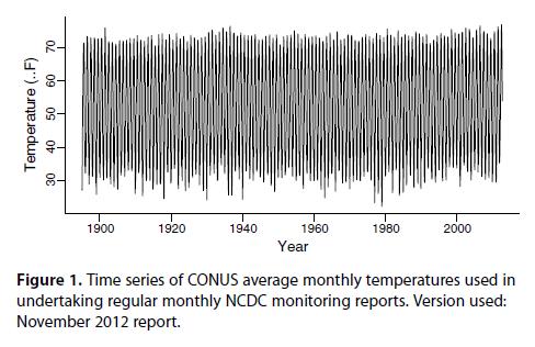
44 Continental US monthly temperatures, Jan 1895 Oct For each month between June 2011 and Sep 2012, the monthly temperature was in the top tercile of all observations for that month up to that point in the time series. Attention was first drawn to this in June 2012, at which point the series of top tercile events was 13 months long, leading to a naïve calculation that the probability of that event was (1/3) 13 = Eventually, the streak extended to 16 months, but ended at that point, as the temperature for Oct 2012 was not in the top tercile. In this study, we estimate the probability of either a 13-month or a 16-month streak of top-tercile events, under various assumptions about the monthly temperature time series. 44

45 45

46 46

47 47

48 48

49 Method Two issues with NOAA analysis: Neglects autocorrelation Ignores selection effect Solutions: Fit time series model ARMA or long-range dependence Use simlulation to determine the probability distribution of the longest streak in 117 years Some of the issues: Selection of ARMA model AR(1) performs poorly Variances differ by month must take that into account Choices of estimation methods, e.g. MLE 0r Bayesian Bayesian methods allow one to take account of parameter estimation uncertainty 49

50 50

51 51

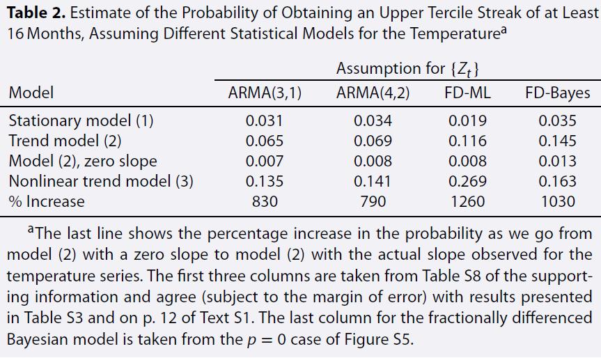
52 Conclusions It s important to take account of monthly varying standard deviations as well as means. Estimation under a high-order ARMA model or fractional differencing lead to very similar results, but don t use AR(1). In a model with no trend, the probability that there is a sequence of length 16 consecutive top-tercile observations somewhere after year 30 in the 117-year time series is of the order of , depending on the exact model being fitted. With a linear trend, these probability rise to something over.05. Include a nonlinear trend, and the probabilities are even higher in other words, not surprising at all. Overall, the results may be taken as supporting the overall anthropogenic influence on temperature, but not to a stronger extent than other methods of analysis. 52

53 I. TIME SERIES ANALYSIS FOR CLIMATE DATA I.a Overview I.b The post-1998 hiatus in temperature trends I.c NOAA s record streak I.d Trends or nonstationarity? II. CLIMATE EXTREMES II.a Extreme value models II.b An example based on track records II.c Applying extreme value models to weather extremes II.d Joint distributions of two of more variables II.e Conclusions, other models, future research 53

54 A Parliamentary Question is a device where any member of the U.K. Parliament can ask a question of the Government on any topic, and is entitled to expect a full answer. 54

55 April 22,

56 56

57 Essence of the Met Office Response Acknowledged that under certain circumstances an ARIMA(3,1,0) without drift can fit the data better than an AR(1) model with drift, as measured by likelihood The result depends on the start and finish date of the series Provides various reasons why this should not be interpreted as an argument against climate change Still, it didn t seem to me (RLS) to settle the issue beyond doubt 57

58 There is a tradition of this kind of research going back some time 58

59 59

60 Summary So Far Integrated or unit root models (e.g. ARIMA(p, d, q) with d = 1) have been proposed for climate models and there is some statistical support for them If these models are accepted, the evidence for a linear trend is not clear-cut Note that we are not talking about fractionally integrated models (0 < d < 2 1 ) for which there is by now a substantial tradition. These models have slowly decaying autocorrelations but are still stationary Integrated models are not physically realistic but this has not stopped people advocating them I see the need for a more definitive statistical rebuttal 60

61 61

62 HadCRUT4 Global Series, Model I : y t y t 1 = ARMA(p, q) (mean 0) Model II : y t = Linear Trend + ARMA(p, q) Model III : y t y t 1 = Nonlinear Trend + ARMA(p, q) Model IV : y t = Nonlinear Trend + ARMA(p, q) Use AICC as measure of fit 62

63 Integrated Time Series, No Trend p q NA

64 Stationary Time Series, Linear Trend p q NA

65 Integrated Time Series, Nonlinear Trend p q NA

66 Stationary Time Series, Nonlinear Trend p q NA

67 Integrated Mean 0 Stationary Linear Trend Series Series Year Year Integrated Nonlinear Trend Stationary Nonlinear Trend Series Series Year Year Four Time Series Models with Fitted Trends 67

68 Integrated Mean 0 Stationary Linear Trend Residual Residual Year Year Integrated Nonlinear Trend Stationary Nonlinear Trend Residual Residual Year Year Residuals From Four Time Series Models 68

69 Integrated Mean 0 Stationary Linear Trend Residual Residual Year Year Integrated Nonlinear Trend Stationary Nonlinear Trend Residual Residual Year Year Residuals From Four Time Series Models 69

70 Conclusions If we restrict ourselves to linear trends, there is not a clearcut preference between integrated time series models without a trend and stationary models with a trend However, if we extend the analysis to include nonlinear trends, there is a very clear preference that the residuals are stationary, not integrated Possible extensions: Add fractionally integrated models to the comparison Bring in additional covariates, e.g. circulation indices and external forcing factors Consider using a nonlinear trend derived from a climate model. That would make clear the connection with detection and attribution methods which are the preferred tool for attributing climate change used by climatologists. 70

71 I. TIME SERIES ANALYSIS FOR CLIMATE DATA I.a Overview I.b The post-1998 hiatus in temperature trends I.c NOAA s record streak I.d Trends or nonstationarity? II. CLIMATE EXTREMES II.a Extreme value models II.b An example based on track records II.c Applying extreme value models to weather extremes II.d Joint distributions of two of more variables II.e Conclusions, other models, future research 71

72 EXTREME VALUE DISTRIBUTIONS X 1, X 2,..., i.i.d., F (x) = Pr{X i x}, M n = max(x 1,..., X n ), Pr{M n x} = F (x) n. For non-trivial results must renormalize: find a n > 0, b n such that { } Mn b n Pr x = F (a n x + b n ) n H(x). a n The Three Types Theorem (Fisher-Tippett, Gnedenko) asserts that if nondegenerate H exists, it must be one of three types: H(x) = exp( e x ), all x (Gumbel) { 0 x < 0 H(x) = exp( x α ) x > 0 (Fréchet) { exp( x H(x) = α ) x < 0 1 x > 0 (Weibull) In Fréchet and Weibull, α > 0. 72

73 The three types may be combined into a single generalized extreme value (GEV) distribution: ( H(x) = exp 1 + ξ x µ ) 1/ξ ψ, (y + = max(y, 0)) where µ is a location parameter, ψ > 0 is a scale parameter and ξ is a shape parameter. ξ 0 corresponds to the Gumbel distribution, ξ > 0 to the Fréchet distribution with α = 1/ξ, ξ < 0 to the Weibull distribution with α = 1/ξ. ξ > 0: long-tailed case, 1 F (x) x 1/ξ, ξ = 0: exponential tail ξ < 0: short-tailed case, finite endpoint at µ ξ/ψ + 73

74 EXCEEDANCES OVER THRESHOLDS Consider the distribution of X conditionally on exceeding some high threshold u: F u (y) = F (u + y) F (u). 1 F (u) As u ω F = sup{x : F (x) < 1}, often find a limit F u (y) G(y; σ u, ξ) where G is generalized Pareto distribution (GPD) G(y; σ, ξ) = 1 ( 1 + ξ y ) 1/ξ σ + Equivalence to three types theorem established by Pickands (1975).. 74

75 The Generalized Pareto Distribution G(y; σ, ξ) = 1 ( 1 + ξ y ) 1/ξ σ +. ξ > 0: long-tailed (equivalent to usual Pareto distribution), tail like x 1/ξ, ξ = 0: take limit as ξ 0 to get G(y; σ, 0) = 1 exp i.e. exponential distribution with mean σ, ( y ), σ ξ < 0: finite upper endpoint at σ/ξ. 75

76 POISSON-GPD MODEL FOR EXCEEDANCES 1. The number, N, of exceedances of the level u in any one year has a Poisson distribution with mean λ, 2. Conditionally on N 1, the excess values Y 1,..., Y N are IID from the GPD. 76

77 Relation to GEV for annual maxima: Suppose x > u. The probability that the annual maximum of the Poisson-GPD process is less than x is Pr{ max Y i x} = Pr{N = 0} + 1 i N = e λ + = exp { n=1 ( λ λ n e λ n! { ξ x u σ ( 1 + ξ x u σ ) 1/ξ }. n=1 ) } 1/ξ n Pr{N = n, Y 1 x,... Y n x} This is GEV with σ = ψ + ξ(u µ), λ = ( 1 + ξ u µ ) 1/ξ ψ. Thus the GEV and GPD models are entirely consistent with one another above the GPD threshold, and moreover, shows exactly how the Poisson GPD parameters σ and λ vary with u. 77

78 ALTERNATIVE PROBABILITY MODELS 1. The r largest order statistics model If Y n,1 Y n,2... Y n,r are r largest order statistics of IID sample of size n, and a n and b n are EVT normalizing constants, then ( Yn,1 b n,..., Y ) n,r b n a n a n converges in distribution to a limiting random vector (X 1,..., X r ), whose density is ( h(x 1,..., x r ) = ψ r exp 1 + ξ x ) 1/ξ r µ ψ ( ξ ) r j=1 log ( 1 + ξ x j µ ψ ). 78

79 2. Point process approach (Smith 1989) Two-dimensional plot of exceedance times and exceedance levels forms a nonhomogeneous Poisson process with Λ(A) = (t 2 t 1 )Ψ(y; µ, ψ, ξ) Ψ(y; µ, ψ, ξ) = ( 1 + ξ y µ ψ ) 1/ξ (1 + ξ(y µ)/ψ > 0). 79

80 Illustration of point process model. 80

81 An extension of this approach allows for nonstationary processes in which the parameters µ, ψ and ξ are all allowed to be timedependent, denoted µ t, ψ t and ξ t. This is the basis of the extreme value regression approaches introduced later Comment. The point process approach is almost equivalent to the following: assume the GEV (not GPD) distribution is valid for exceedances over the threshold, and that all observations under the threshold are censored. Compared with the GPD approach, the parameterization directly in terms of µ, ψ, ξ is often easier to interpret, especially when trends are involved. 81

82 GEV log likelihood: l Y (µ, ψ, ξ) = N log ψ ESTIMATION i ( ( ) 1 ξ ξ Y i µ ψ i ) 1/ξ provided 1 + ξ(y i µ)/ψ > 0 for each i. log ( 1 + ξ Y i µ ψ ) Poisson-GPD model: l N,Y (λ, σ, ξ) = N log λ λt N log σ provided 1 + ξy i /σ > 0 for all i. ( ξ ) N i=1 log ( 1 + ξ Y i σ ) Usual asymptotics valid if ξ > 1 2 (Smith 1985) 82

83 Bayesian approaches An alternative approach to extreme value inference is Bayesian, using vague priors for the GEV parameters and MCMC samples for the computations. Bayesian methods are particularly useful for predictive inference, e.g. if Z is some as yet unobserved random variable whose distribution depends on µ, ψ and ξ, estimate Pr{Z > z} by Pr{Z > z; µ, ψ, ξ}π(µ, ψ, ξ Y )dµdψdξ where π(... Y ) denotes the posterior density given past data Y 83

84 I. TIME SERIES ANALYSIS FOR CLIMATE DATA I.a Overview I.b The post-1998 hiatus in temperature trends I.c NOAA s record streak I.d Trends or nonstationarity? II. CLIMATE EXTREMES II.a Extreme value models II.b An example based on track records II.c Applying extreme value models to weather extremes II.d Joint distributions of two of more variables II.e Conclusions, other models, future research 84

85 Plots of women s 3000 meter records, and profile log-likelihood for ultimate best value based on pre-1993 data. 85

86 Example. The left figure shows the five best running times by different athletes in the women s 3000 metre track event for each year from 1972 to Also shown on the plot is Wang Junxia s world record from Many questions were raised about possible illegal drug use. We approach this by asking how implausible Wang s performance was, given all data up to Robinson and Tawn (1995) used the r largest order statistics method (with r = 5, translated to smallest order statistics) to estimate an extreme value distribution, and hence computed a profile likelihood for x ult, the lower endpoint of the distribution, based on data up to 1992 (right plot of previous figure) 86

87 Alternative Bayesian calculation: (Smith 1997) Compute the (Bayesian) predictive probability that the 1993 performance is equal or better to Wang s, given the data up to 1992, and conditional on the event that there is a new world record. 87

88 > yy=read.table( C:/Users/rls/r2/d/evt/marathon/w3000.txt,header=F) > r=5 >

89 > # likelihood function (compute NLLH - defaults to 10^10 if parameter values > # infeasible) - par vector is (mu, log psi, xi) > lh=function(par){ + if(abs(par[2])>20){return(10^10)} + #if(abs(par[3])>1){return(10^10)} + if(par[3]>=0){return(10^10)} + mu=par[1] + psi=exp(par[2]) + xi=par[3] + f=0 + for(i in 9:21){ + f=f+r*par[2] + s1=1+xi*(mu-yy[i,6])/psi + if(s1<=0){return(10^10)} + s1=-log(s1)/xi + if(abs(s1)>20){return(10^10)} + f=f+exp(s1) + for(j in 2:6){ + s1=1+xi*(mu-yy[i,j])/psi + if(s1<=0){return(10^10)} + f=f+(1+1/xi)*log(s1) + }} + return(f) + } 89

90 > # trial optimization of likelihood function > par=c(520,0,-0.01) > lh(par) [1] > > par=c(510,1,-0.1) > lh(par) [1] > > opt1=optim(par,lh,method="nelder-mead") > opt2=optim(par,lh,method="bfgs") > opt3=optim(par,lh,method="cg") > opt1$par [1] > opt2$par [1] > opt3$par [1] > opt1$value [1] > opt2$value [1] > opt3$value [1] > 90

91 > > # MLE of endpoint (intepreted as smallest possible running time) > > opt1$par[1]+exp(opt1$par[2])/opt1$par[3] [1] > opt2$par[1]+exp(opt2$par[2])/opt2$par[3] [1] > > # now do more through optimization and prepare for MCMC > par=c(520,0,-0.01) > opt2=optim(par,lh,method="bfgs",hessian=t) > library(mass) > A=ginv(opt2$hessian) > sqrt(diag(a)) [1] > eiv=eigen(a) > V=eiv$vectors > V=V %*% diag(sqrt(eiv$values)) %*% t(v) 91

92 > # MCMC - adjust nsim=total number of simulations, > par=opt2$par > nsim= > nsave=1 > nwrite=100 > del=1 > lh1=lh(par) > parsim=matrix(nrow=nsim/nsave,ncol=3) > accp=rep(0,nsim) > for(isim in 1:nsim){ + # Metropolis update step + parnew=par+del*v %*% rnorm(3) + lh2=lh(parnew) + if(runif(1)<exp(lh1-lh2)){ + lh1=lh2 + par=parnew + accp[isim]=1 + } + if(nsave*round(isim/nsave)==isim){ + parsim[isim/nsave,]=par + write(isim, C:/Users/rls/mar11/conferences/NCSUFeb2015/counter.txt,ncol=1) + } + if(nwrite*round(isim/nwrite)==isim){ + write(parsim, C:/Users/rls/mar11/conferences/NCSUFeb2015/parsim.txt,ncol=1)}} 92

93 > # results from presaved MCMC output > parsim1=matrix(scan( C:/Users/rls/mar11/conferences/NCSUFeb2015/parsim1.txt ),nro Read items > parsim=parsim1[(length(parsim1[,1])/2+1):length(parsim1[,1]),] > s1=1+parsim[,3]*(parsim[,1] )/exp(parsim[,2]) > s1[s1<0]=s1 > s1[s1>0]=1-exp(-s1[s1>0]^(-1/parsim[s1>0,3])) > s2=1+parsim[,3]*(parsim[,1] )/exp(parsim[,2]) > s2[s2<0]=0 > s2[s2>0]=1-exp(-s2[s2>0]^(-1/parsim[s2>0,3])) > mean(s2/s1) [1] > mean(s2==0) [1] > quantile(s2/s1,c(0.5,0.9,0.95,0.975,0.995)) 50% 90% 95% 97.5% 99.5% > endp=parsim[,1]+exp(parsim[,2])/parsim[,3] > sum(endp<486.11)/length(endp) [1] > plot(density(endp[endp>460])) 93

94 94

95 I. TIME SERIES ANALYSIS FOR CLIMATE DATA I.a Overview I.b The post-1998 hiatus in temperature trends I.c NOAA s record streak I.d Trends or nonstationarity? II. CLIMATE EXTREMES II.a Extreme value models II.b An example based on track records II.c Applying extreme value models to weather extremes II.d Joint distributions of two of more variables II.e Conclusions, other models, future research 95

96 96

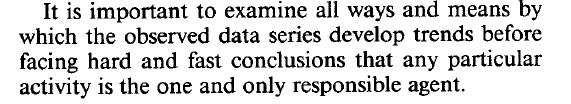
97 Motivating Question: Concern over increasing frequency of extreme meteorological events Is the increasing frequency a result of anthropogenic influence? How much more rapidly with they increase in the future? Focus on three specific events: heatwaves in Europe 2003, Russia 2010 and Central USA 2011 Identify meteorological variables of interest JJA temperature averages over a region Europe 10 o W to 40 o E, 30 o to 50 o N Russia 30 o to 60 o E, 45 o to 65 o N Central USA 90 o to 105 o W, 25 o to 45 o N Probabilities of crossing thresholds respectively 1.92K, 3.65K, 2.01K in any year from 1990 to

98 Data Climate model runs have been downloaded from the WCRP CMIP3 Multi-Model Data website ( Three kinds of model runs: Twentieth-century Pre-industrial control model runs (used a proxy for natural forcing) Future projections (A2 scenario) We also took observational data (5 o 5 o gridded monthly temperature anomalies) from the website of the Climate Research Unit of the University of East Anglia ( Had- CRUT3v dataset) 98

99 Number Model Control runs 20C runs A2 runs 1 bccr bcm cccma cgcm cnrm cm csiro mk gfdl cm giss model e r ingv echam inmcm ipsl cm miroc3 2 medres mpi echam mri cgcm2 3 2a ncar ccsm ukmo hadcm List of climate models, including numbers of runs available under three scenarios 99

100 (a) Europe JJA Temperatures Anomaly Year 100

101 (b) Russia JJA Temperatures Anomaly Year 101

102 (c) Central USA JJA Temperatures Anomaly Year 102

103 Analysis of Observational Data Key tool: Generalized Extreme Value Distribution (GEV) Three-parameter distribution, derived as the general form of limiting distribution for extreme values (Fisher-Tippett 1928, Gnedenko 1943) µ, σ, ξ known as location, scale and shape parameters ξ > 0 represents long-tailed distribution, ξ < 0 short-tailed Formula: Pr{Y y} = exp [ { 1 + ξ ( y µ σ )} ] 1/ξ

104 Peaks over threshold approach implies that the GEV can be used generally to study the tail of a distribution: assume GEV holds exactly above a threshold u and that values below u are treated as left-censored Time trends by allowing µ, σ, ξ to depend on time Example: Allow µ t = β 0 + K k=1 β k x kt where {x kt, k = 1,..., K, t = 1,..., T } are spline basis functions for the approximation of a smooth trend from time 1 to T with K degrees of freedom Critical questions: Determination of threshold and K Estimating the probability of exceeding a high value such as 1.92K 104

105 Application to Temperature Series GEV with trend fitted to three observational time series Threshold was chosen as fixed quantile 75th, 80th or 85th percentile AIC was used to help select the number of spline basis terms K Estimate probability of extreme event by maximum likelihood (MLE) or Bayesian method Repeat the same calculation with no spline terms Use full series or part? Examine sensitivity to threshold choice through plots of the posterior densities. 105

106 K Europe Russia Texas Threshold 75% 80% 85% AIC values for different values of K, at three different thresholds, for each dataset of interest. In each column, the smallest three AIC values are indicated in red, green and blue respectively. 106

107 Dataset Endpoint K Threshold MLE Posterior Posterior Quantiles Mean Europe % Europe % Europe % Europe % Russia % Russia % Russia % Russia % CentUSA % CentUSA % CentUSA % CentUSA % Results of extreme value analysis applied to observational datasets. For three datasets (Europe, Russia, Central USA), different choices of the endpoint of the analysis, spline degrees of freedom K, and threshold, we show the maximum likelihood estimate (MLE) of the probability of the extreme event of interest, as well as the posterior mean and three quantiles of the posterior distribution. 107

108 (a) Europe JJA Temperatures (b) Russia JJA Temperatures Anomaly Anomaly Year Year (c) Central USA JJA Temperatures Anomaly Year Plot of three time series for , with fitted trend curves. 108

109 Europe Russia CentUSA Density Density Density BLOTEP BLOTEP BLOTEP Europe No Trend Russia No Trend CentUSA No Trend Density Density Density BLOTEP BLOTEP BLOTEP Posterior densities of the BLOTEP, with (top) and without (bottom) spline-based trends. Based on 80% (solid curve), 75% (dashed) and 85% (dot-dashed) thresholds. 109

110 Summary So Far: Estimate extreme event probabilities by GEV with trends Bayesian posterior densities best way to describe uncertainty Two major disadvantages: No way to distinguish anthropogenic climate change effects from other short-term fluctations in the climate (El Niños and other circulation-based events; the 1930s dustbowl in the US) No basis for projecting into the future It might seem that the way to do future projections is simply to rerun the analysis based on climate model data instead of observations. However, this runs into the scale mismatch problem. 110

111 Model GFDL, Run 1, Europe Model GISS, Run 1, Europe Anomaly Anomaly Year Year Model NCAR, Run 1, Europe Model HADCM3, Run 1, Europe Anomaly Anomaly Year Year Scale mismatch: 4 model runs (range of observations in red). 111

112 Model GFDL, Run 1, Russia Model GISS, Run 1, Russia Anomaly Anomaly Year Year Model NCAR, Run 1, Russia Model HADCM3, Run 1, Russia Anomaly Anomaly Year Year Scale mismatch: 4 model runs (range of observations in red). 112

113 Model GFDL, Run 1, Central USA Model GISS, Run 1, Central USA Anomaly Anomaly Year Year Model NCAR, Run 1, Central USA Model HADCM3, Run 1, Central USA Anomaly Anomaly Year Year Scale mismatch: 4 model runs (range of observations in red). 113

114 I. TIME SERIES ANALYSIS FOR CLIMATE DATA I.a Overview I.b The post-1998 hiatus in temperature trends I.c NOAA s record streak I.d Trends or nonstationarity? II. CLIMATE EXTREMES II.a Extreme value models II.b An example based on track records II.c Applying extreme value models to weather extremes II.d Joint distributions of two of more variables II.e Conclusions, other models, future research 114

115 Example 1. Herweijer and Seager (2008) argued that the persistence of drought patterns in various parts of the world may be explained in terms of SST patterns. One of their examples (Figure 3 of their paper) demonstrated that precipitation patterns in the south-west USA are highly correlated with those of a region of South America including parts of Uruguay and Argentina. I computed annual precipitation means for the same regions, that show the two variables are clearly correlated (r=0.38; p.0001). The correlation coefficient is lower than that stated by Herweijer and Seager (r=0.57) but this is explained by their use of 6-year moving average filter, which naturally increases the correlation. Our interest here: look at dependence in lower tail probabilities Transform to unit Fréchet distribution (small values of precipitation corresponding to large values on Frchet scale) 115

116 Urug Arg Rain (mm/mon) A Transformed Urug Arg Rain A A A SW USA Rain (mm/mon) Transformed SW USA Rain Figure 1. Left: Plot of USA annual precipitation means over latitudes o N, longitudes o W, against Argentina annual precipitation means over latitudes o S, longitudes o W, Right: Same data with empirical transformation to unit Fréchet distribution. Data from gridded monthly precipitation means archived by the Climate Research Unit of the University of East Anglia. 116

117 Example 2. Lau and Kim (2012) have provided evidence that the 2010 Russian heatwave and the 2010 Pakistan floods were derived from a common set of meteorological conditions, implying a physical dependence between these very extreme events. Using the same data source as for Example 1, I have constructed summer temperature means over Russia and precipitation means over Pakistan corresponding to the spatial areas used by Lau and Kim. Scatterpolt of raw data and unit Fréchet transformation value approximated an outlier for temperature but not for precipitation. 117

118 Pakistan Rain (mm/mon) * Transformed Pakistan Rain Russian Temperature (deg C) Transformed Russian Temperature Figure 2. Left: Plot of JJA Russian temperature means against Pakistan JJA precipitation means, Right: Same data with empirical transformation to unit Fréchet distribution. Data from CRU, as in Figure 1. The Russian data were averaged over o N, o E, while the Pakistan data were averaged over o N, o E, same as in Lau and Kim (2012). 118

119 Methods Focus on the proportion by which the probability of a joint exceedance is greater than what would be true under independence. Method: Fit a joint bivariate model to the exceedances above a threshold on the unit Fréchet scale Two models: Classical logistic dependence model (Gumbel and Mustafi 1967; Coles and Tawn 1991) The η-asymmetric logistic model (Ramos and Ledford 2009) 119

120 Logistic Model Ramos-Ledford Model Estimate 90% CI Estimate 90% CI 10-year 2.7 (1.2, 4.2) 2.9 (1.2, 5.0) 20-year 4.7 (1.4, 7.8) 4.9 (1.2, 9.6) 50-year 10.8 (2.1, 18.8) 9.9 (1.4, 23.4) Table 1. Estimates of the increase in probability of a joint extreme event in both variables, relative to the probability under independence, for the USA/Uruguay-Argentina precipitation data. Shown are the point estimate and 90% confidence interval, under both the logistic model and the Ramos-Ledford model. Logistic Model Ramos-Ledford Model Estimate 90% CI Estimate 90% CI 10-year 1.01 (1.00, 1.01) 0.33 (0.04, 1.4) 20-year 1.02 (1.00, 1.03) 0.21 (0.008, 1.8) 50-year 1.05 (1.01, 1.07) 0.17 (0.001, 2.9) Table 2. Similar to Table 1, but for the Russia-Pakistan dataset. 120

121 Conclusions The USA Argentina precipitation example shows clear dependence in the lower tail, though the evidence for that rests primarily on three years data In contrast, the analysis of Russian temperatures and Pakistan rainfall patterns shows no historical correlation between those two variables Implications for future analyses: the analyses also show the merits of the Ramos-Ledford approach to bivariate extreme value modeling. The existence of a parametric family which is tractable for likelihood evaluation creates the possibility of constructing hiterarchical models for these problems. 121

122 I. TIME SERIES ANALYSIS FOR CLIMATE DATA I.a Overview I.b The post-1998 hiatus in temperature trends I.c NOAA s record streak I.d Trends or nonstationarity? II. CLIMATE EXTREMES II.a Extreme value models II.b An example based on track records II.c Applying extreme value models to weather extremes II.d Joint distributions of two of more variables II.e Conclusions, other models, future research 122

123 At least three methodological extensions, all of which are topics of active research: 1. Models for multivariate extremes in > 2 dimensions 2. Spatial extremes: max-stable process, different estimation methods (a) Composite likelihood method (b) Open-faced sandwich approach (c) Approximations to exact likelihood, e.g. ABC method 3. Hierarchical models for bivariate and spatial extremes? 123