ECOLOGICAL STATISTICS: Analysis of Capture-Recapture Data

Transcription

1 ECOLOGICAL STATISTICS: Analysis of Capture-Recapture Data Rachel McCrea and Byron Morgan National Centre for Statistical Ecology, University of Kent, Canterbury.

2 Outline 1. Introduction 2. Estimating abundance 3. Survival estimation 4. Model selection 5. Complex models 6. Parameter redundancy 7. State-space modelling 8. Bayesian analysis

3 Outline: Computer practicals 1. Introduction 2. Estimating abundance: EstimateN 3. Survival estimation: Mark and RMark 4. Model selection: Eagle 5. Complex models 6. Parameter redundancy: Maple 7. State-space modelling: Kalm 8. Bayesian analysis: WinBUGs

4 SECTION 1 INTRODUCTION

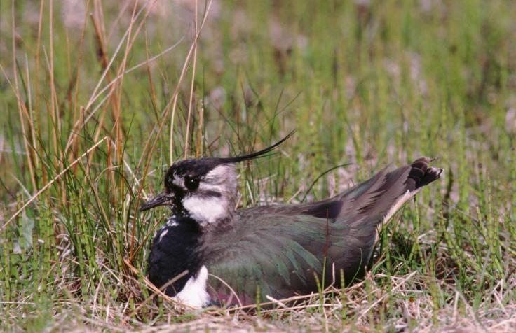
5 Introduction We are seeing changes in wild animal populations worldwide. In Britain there are notable declines in sparrows (Passer domesticus), lapwing(vanellus vanellus), spotted fly-catcher (Muscicapa striata), etc. Effects of global warming and changes in farming practice

6 Motivation Importance of anthropogenic change: 6 th mass extinction. 2010: The year of biodiversity

7

8 Large literature Papers in journals such as: Biometrics, JABES, JRSS, J.An. Ecology. Ecology, Oikos, J. Wildlife Management, Can. J. Fish. Aq. Sci., Meth. Ecol. Evol., Epidemiology Books: Seber (1982), Williams et al (2002), King et al (2009), McCrea and Morgan (2011) Web-sites: Computer packages: DISTANCE, MARK, E-SURGE, Presence.

9 Statistical Ecology; capture-recapture Estimation of population sizes Estimation of important demographic rates (cf human demography): Survival Productivity Movement Dealing with complexity Use of capture-recapture methods; started with H.C. Mortensen, 1899.

10 Recent Kent projects Jose multi-species survival; synchrony; IoM Guru Occupancy; tigers, Sumatra Beth Benthic organisms; diversity; trawling Rachel Model selection; goodness-of-fit; multi-state models Diana Parameter redundancy Lauren Spatio-temoral capture-recapture; cheetahs; missing time-varying individual covariates. Martin Meercat survival; closed population sizes Teresa Over-wintering wildfowl David Demography of the lizard orchid Dan local weather; use of lasso for variable selection Achaz Ibex; winter snow vs. reproductive senescence Eleni Stop-over models; demographic uses Takis Integrated population modelling; batch marking Ben Parameter redundancy

11 Marking We obtain information on survival from studying previously marked animals. These may be observed again alive or dead. It is assumed that marking does not affect behaviour (See J. An. Ec. 2005).

12 Shag rings, Isle of May: José

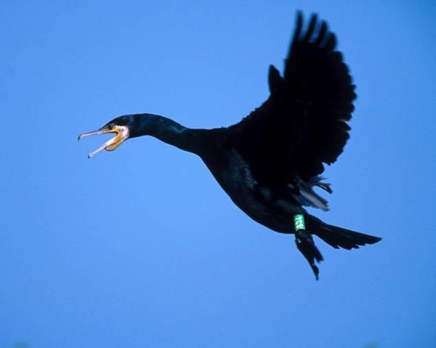
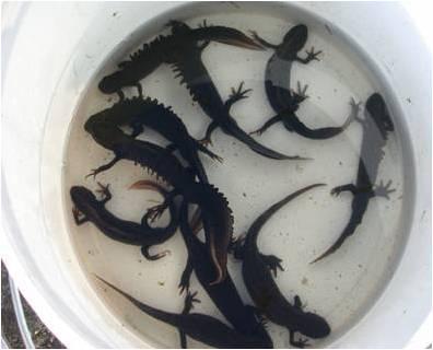
13 Identification/recapture/resighting of Cormorant, Phalacrocorax carbo sinensis, and great crested newt, Titurus cristatus

14 Further examples

15 Practicalities

16 Try again

17 Deer collars on Rum

18 Alternatives Radio tracking DNA Note possibility of errors Problems with ring loss

19 Fecundity The key demographic processes involve survival, reproduction and movement. We shall be mainly concerned with the estimation of survival. Estimation of fecundity can be challenging, but is typically easier than the estimation of survival. For example, Cory s shearwaters lay just one egg.

20 The Classical Approach For a given data set we consider a family of alternative probability models. Each model may be fitted by means of optimising some criterion, for example by maximising a likelihood over the parameter space. Many parameters may be involved. Models may be compared in terms of maximised likelihoods, or information criteria, such as the AIC or BIC. Usually a single best model is selected to represent the data, in terms of the model parameter estimates and estimates of their precision.

21 Classical continued Models may be averaged, using model weights derived from AICs. Cf. Bayesian approach. Model averaging, in general, should not be uncritical, as differences resulting from different models should be understood (McAllister). Computing is usually done using packages such as MARK or E-SURGE. It is necessary to interface with packages in order to make model specifications. For example one can use parameter-index matrices, PIMs. Diagnostics include looking at residuals of various kinds, and constructing tests of goodness-of-fit.

22 The Bayesian approach Brooks Catchpole and Morgan, (2000) Bayesian Animal Survival Estimation, Statistical Science, 15, King, Morgan, Gimenez and Brooks (2009) Bayesian Analysis for Population Ecology. Chapman & Hall/CRC, London.

23 SECTION 2 ESTIMATING ABUNDANCE

24 Estimating Abundance Standard estimators The importance of heterogeneity Illustrations from different areas

25 How many individuals? From skinks..

26 ..to taxis: need for individual identification

27 Medical and social applications How many French people are there (Laplace)? How many illegal firearms? How many drugs users? Eg., in a Bangkok study of drug users, 7062 individuals had hospital encounters, with f 1 =2955, f 2 =1186, f 3 =803, How many traffic offences?

28 How many animals? The Lincoln-Petersen estimate is given by the solution in N to the equation below, where a first sample of n 1 animals are captured and marked, and then a later sample resulted in n 2 animals, of which m 2 were marked.

29 The Schnabel census: data Repetition of the sampling scheme results in data of the form below hares taxis voles voles chips

30 The Horvitz-Thompson estimate

31 Horvitz-Thompson

32 Likelihood for the Schnabel census The general form of the likelihood is given by where N is the population size, denotes the model parameters, p j now denotes the probability an animal is caught j times, f j is the number of animals caught j times, k is the number of sampling occasions and D is the number of distinct animals caught.

33 Violation of assumptions This approach is harder than it seems because, amongst other things, animals differ in their re-capture rates. Nevertheless, this remains an area of active research.

34 Models: the bias due to unmodelled heterogeneity can be severe! Example: Ayre (1962) estimated an anthill population to be 109 when there were known to be 3,000 ants in it. Ayre, L.G Problems in using the Lincoln index for estimating the size of ant colonies (Hymenopter formicidae). J.N.Y. Ent. Soc. 70:

35 Two recent approaches to unobservable heterogeneity Finite Mixture models 1 : approximate the distribution of p using a mixture of a few ps (conceptually from a few sub-populations). Continuous (or infinite mixture) models 2 : Model the distribution of p using some flexible continuous distribution (e.g. Beta) 1 Pledger, S Unified maximum likelihood estimates for closed capture-recapture models using mixtures. Biometrics 56: Dorazio, R.M. and Royle, J.A Mixture models for estimating the size of a closed population when capture rates vary among individuals. Biometrics 59:

36 Alternative mixture models Infinite mixture model Finite mixture model (mixture of 2 types) f(p) 0 p 1 p 1 p 2

37 Types of mark-recapture model M 0 : No heterogeneity M t : Capture probabilities vary with time (occasion) M b : Capture probabilities depend on behaviour (trap-shy or trap-happy) M h : Capture probabilities are heterogeneous (vary between individuals) And combinations: M tb, M th, M bh, M tbh

38 New mixture model We proposed a mixture of binomial and beta-binomial distributions for estimating the size of closed populations. The new model includes discrete (two populations) and infinite mixtures, used for the recapture probability by Pledger, and Dorazio and Royle, as special cases

39 Modelling heterogeneity of recapture p j / a a j(1- a ) k -j p j / r (+r ) r (1-+r )/ r (1+r ) j Be p j / { j (1-) k-j + (1-) j Be }

40 Alternatives Nonparametric (E and Q), and the logistic-normalbinomial model:

41 Illustration of different precision for a single data set, where it is thought N=102. Model N 95% Profile interval Beta-bin Bins Bin + Beta-bin E Q

42 Change to beta parameters For the beta-binomial model, we have =0.40, =3.41. For the new mixture we have =1.30, =5.95.

43 Modelling the parameter p near zero Thus the new model allows flexible modelling of the probability of recapture, p, near zero, which is important for estimating N. Shown in the next graph is how the logistic-normal-binomial, beta and the beta component of the new mixture can differ in modelling p near zero, for a particular data set.

44 Different capture probabilities near zero.

45 Results: illustrative comparisons of model fits: -max log-lik., values. Data Binomial Betabinomial 2 Bins Bin + Beta-bin House mice Skinks Wood mice Taxicabs Squirrels

46 Illustrative coverage, 95% profile CI True model Fitted model Coverage Beta-bin Binomial Beta-bin Beta-bin Beta-bin 2 Bins Beta-bin Bin + Beta-bin Bins Binomial Bins Beta-bin Bins 2 Bins Bins Bin + Beta-bin 0.955

47 Further work Mix a binomial with a logistic-normalbinomial, in order to include also the cases of time and behavioural response. Extend mixture to modelling survival and site-occupancy models. Include covariates.

48 SECTION 3 SURVIVAL ESTIMATION

49 Survival estimation 3.1: Analysing recovery data 3.2: Capture-recapture data 3.3: Integrated recaptures and recoveries

50 Analysing Recovery Data Cohort of individuals marked and rereleased into the population When individuals die, they may be recovered dead; or their rings/marks may be recovered. Form encounter histories for each individual: 1: time individual marked 2: time individual recovered dead

51 Recovery Data R i : number of marked individuals released at occasion t i d ij : number of individuals released at occasion ti and recovered dead in the time interval (t j-1,t j ) Consider a 4 encounter occasion study, then individuals released at time t 1 can be summarised as: R 1 d 1,2 d 1,3 d 1,4 R 1 -d 1,2 -d 1,3 -d 1,4

52 Multinomial Distribution R 1 d 1,2 d 1,3 d 1,4 R 1 -d 1,2 -d 1,3 -d 1,4 Defining: i : probability an individual alive at occasion t i survives until occasion t i+1 i : probability an individual who dies between occasion t i and t i+1 is recovered (or has its ring/tag) and reported R 1 (1-1 ) 1 1 (1-2 ) (1-3 ) 3 1 X j Pr(d i;j )

53 Product Multinomial Consider a general m-array for a 4 occasion recovery study Releases Recovery Occasion Never Recovered R 1 d 1;2 d 1;3 d 1;4 d 1;1 R 2 d 2;3 d 2;4 d 2;1 R 3 d 3;4 d 3;1 where d i;1 = R i X j d i;j

54 Product Multinomial Then the corresponding probabilities are Releases Recovery Occasion Never Recovered R 1 (1 Á 1 ) 1 Á 1 (1 Á 2 ) 2 Á 1 Á 2 (1 Á 3 ) 3 1 P j Pr(d 1;j) R 2 (1 Á 2 ) 2 Á 2 (1 Á 3 ) 3 1 P j Pr(d 2;j) R 3 (1 Á 3 ) 3 1 P j Pr(d 3;j) Assuming independence between release cohorts, the log-likelihood function is then defined by log(l) = constant + X i X d i;j log(pr(d i;j )) j

55 Example: Mallards, Anas platyrhynchos Year of No. Year of recovery (-1962) ringing ringed

56 MLEs: Mallard model (.),(t) Parameter MLE SE Á( )

57 Freeman-Morgan Model For bird populations, first-year survival is often dramatically different from adult survival If individuals marked as nestlings, then it is possible to adapt the model to incorporate agedependent parameters

58 Freeman-Morgan Model Introduce model notation x/y/z: x: first-year-survival probability y: adult-survival probability z: recovery probability Possible parameter dependencies c: constant t: time-dependence a k : age-dependence up to age k v: covariate-dependence (see later section)

59 Model c/c/t (1): first-year survival probability (a): adult survival probability Releases Recovery Occasion Never Recovered R 1 (1 Á(1)) 1 Á(1)(1 Á(a)) 2 Á(1)Á(a)(1 Á(a)) 3 1 P j Pr(d 1;j) R 2 (1 Á(1)) 2 Á(1)(1 Á(a)) 3 1 P j Pr(d 2;j) R 3 (1 Á(1)) 3 1 P j Pr(d 3;j)

60 More general age-dependence P r(d ij (a)) = 8 >< >: 0 i > j (1 Á j (a)) j(a) i = j Q j 1 k=1 Á k(a + k i) (1 Á j (a + j i)) j(a + j i) i < j

61 Example: Mallards (marked as young) Year of No. Year of recovery (-1962) ringing ringed

62 MLEs: Mallards t/c/t model Parameter MLE SE Parameter MLE SE Á 1 (1) Á 2 (1) Á 3 (1) Á 4 (1) Á 5 (1) Á 6 (1) Á 7 (1) Á 8 (1) Á 9 (1) Á(2+)

63 Extensions Modelling ring-recovery data when the number of ringed individuals is not known (Brown, 2010) Modelling adult-survival heterogeneity (Besbeas et al, 2009) Mixture models for modelling agedependent survival (McCrea et al, 2010)

64 References Besbeas et al (2009) in Modelling Demographic processes in marked populations. pp Brown (2010) PhD Thesis, University of Kent Brownie et al (1985) Statistical inference from band recovery data A handbook. Freeman and Morgan (1992) Biometrics, 48: McCrea et al, (2010) Submitted.

65 Capture-recapture data Suppose now, that instead of recovering dead individuals, attempts are made instead to recapture live individuals 1: initial capture and subsequent live recaptures Examples:

66 Recapture M-array Number Released Recaptured t 2 Recaptured t 3 Recaptured t 4 Never Recaptured R 1 m 12 m 13 m 14 R 1 -m 12 -m 13 -m 14 R 2 m 23 m 24 R 2 -m 23 -m 24 R 3 m 34 R 3 -m 34 R i : Number of individuals released in year t i m ij : Number of individuals released in year t i and next recaptured in year t j

67 Encounter Histories to M-arrays Number Released Recaptured t 2 Recaptured t 3 Recaptured t 4 Never Recaptured R 1 m 12 m 13 m 14 R 1 -m 12 -m 13 -m 14 R 2 m 23 m 24 R 2 -m 23 -m 24 R 3 m 34 R 3 -m R i : newly marked individuals AND re-released individuals

68 Singlesite Probabilities Number Released Recaptured t Never 2 Recaptured t 3 Recaptured t 4 Recaptured R 1 1 p 2 1 (1-p 2 ) 2 p 3 1 (1-p 2 ) 2 (1-p 3 ) 3 p 4 1-probabilities R 2 2 p 3 2 (1-p 3 ) 3 p 4 1-probabilities R 3 3 p 4 1-probabilities i : probability an animal alive at time t i survives to time t i+1 p i+1 : probability an animal alive at time t i+1 is recaptured at time t i+1 Cormack-Jolly-Seber Model: (t),p(t)

69 Example: Great Crested Newts Mark-recapture data collected between 1995 and 2006 Population of Great crested newts, Tristurus cristatus, close to the University of Kent campus. Meta-population studied over four groups of ponds Best model: (t),p(pond)

70

71

72 Wellcourt Study Site

73 Great Crested Newts: (t),p(pond) What is causing this temporal variation? Griffiths et al (2010) Garden Pond: P = ( ) Swimming Pool: p = ( ) Snake Pond: p = ( ) Pylon Pond: p = ( )

74 Extensions General age and time-dependent models Individual heterogeneity (random effect) models (Gimenez and Choquet, 2010) Incorporation of behavioural traits, e.g. trap-response

75 References Cormack (1964) Biometrika, 51: Gimenez and Choquet (2010) Ecology, 91: Griffiths et al (2010) Biological Conservation, 143: Jolly (1965) Biometrika, 52: Seber (1965) Biometrika, 52:

76 Joint recapture and recovery models What if both recapture and recovery data are collected on the same individuals?

77 Sufficient Statistics Catchpole, Freeman, Morgan and Harris (1998) Integrated Recovery/Recapture Data Analysis. Biometrics. 54, General cohort/age/time-dependence Assumes no emigration Alternative modelling approach in Barker (1997,1999).

78 CM Parameters (Time-dependent Model) ϕ j : probability an animal alive at time t j survives until time t j+1 ; λ j : probability an animal which dies in the interval (t j,t j+1 ), has its death reported; p j : probability an animal alive at time t j, is captured at t j.

79 CM Likelihood Construction : Live recapture 2: Dead recovery

80 CM Likelihood Construction ϕ 1 p 2 (1-ϕ 2 )λ 2 ϕ 1 (1-p 2 )ϕ 2 (1-p 3 )(1-ϕ 3 )λ 3 ϕ 1 p 2 ϕ 2 p 3 ϕ 3 p 4 ϕ 4 p 5 χ 5 ϕ 1 p 2 χ 2 χ j: probability an animal alive at time t j is not seen again, alive or dead after t j

81 CM Likelihood Construction ϕ 1 p 2 (1-ϕ 2 )λ 2 ϕ 1 (1-p 2 )ϕ 2 (1-p 3 )(1-ϕ 3 )λ 3 ϕ 1 p 2 ϕ 2 p 3 ϕ 3 p 4 ϕ 4 p 5 χ 5 ϕ 1 p 2 χ 2 Known survival... 1 j s j s1

82 CM Likelihood Construction ϕ 1 p 2 (1-ϕ 2 )λ 2 ϕ 1 (1-p 2 )ϕ 2 (1-p 3 )(1-ϕ 3 )λ 3 ϕ 1 p 2 ϕ 2 p 3 ϕ 3 p 4 ϕ 4 p 5 χ 5 ϕ 1 p 2 χ 2 Disappearing individuals... 1 j (1 j ) j j (1 (1 pj 1) j 1)

83 CM Likelihood Construction ϕ 1 p 2 (1-ϕ 2 )λ 2 ϕ 1 (1-p 2 )ϕ 2 (1-p 3 )(1-ϕ 3 )λ 3 ϕ 1 p 2 ϕ 2 p 3 ϕ 3 p 4 ϕ 4 p 5 χ 5 ϕ 1 p 2 χ 2 Recaptures...

84 CM Likelihood Construction ϕ 1 p 2 (1-ϕ 2 )λ 2 ϕ 1 (1-p 2 )ϕ 2 (1-p 3 )(1-ϕ 3 )λ 3 ϕ 1 p 2 ϕ 2 p 3 ϕ 3 p 4 ϕ 4 p 5 χ 5 ϕ 1 p 2 χ 2 Death and recovery...

85 CM Likelihood Construction ϕ 1 p 2 (1-ϕ 2 )λ 2 ϕ 1 (1-p 2 )ϕ 2 (1-p 3 )(1-ϕ 3 )λ 3 ϕ 1 p 2 ϕ 2 p 3 ϕ 3 p 4 ϕ 4 p 5 χ 5 ϕ 1 p 2 χ 2 Non-captures...

86 CM Sufficient Statistics D(j): number of animals recovered dead in the interval (t j,t j+1 ); V(j): number of animals captured or recaptured at t j and not seen again during the study; W(j): number of animals recaptured at t j+1 ; Z(j): number of animals not recaptured at t j+1 but encountered later either dead or alive

87 CM Likelihood Construction T j T j j Z j j W j j V j j T j j D j j j p p L ) ( 1 ) ( 1 ) ( 1 1 ) ( ) (1 ) 1 ( Note that many animals are counted in both V(j) and W(j) Sufficient statistics D, V, W and Z are therefore not independent multinomials Time-dependence structure given here, CM form completely general.

88 SECTION 4 MODEL ASSESSMENT

89 Model Selection Comparing models: which one is best? AIC/LRT tests Step-wise approaches using score tests Goodness-of-fit Absolute goodness-of-fit tests Diagnostic assessment departure from model assumptions

90 Model Selection using AIC Return to the Great crested newt example presented earlier Cormack-Jolly-Seber model: Constant or time-dependent parameters Pond specific parameters Weather covariates?

91 AIC Akaike's information criterion is de ned by: AIC = 2 log L(^µ j x) + 2K where L( j x) is the likelihood function given the observed data x, ^µ are the MLEs of the components of parameter µ and K is the size of ^µ, which can be interpreted as the number of estimable parameters of the model.

92 AIC The smaller the AIC, the smaller the -2logL, which will signify a comparatively better fitting model. Of course the number of parameters is also discriminated against within the information criterion, and the AIC can be used to rank models in a model set. Models not in the set remain out of consideration. AIC is useful in selecting the best model in the set; however, if all models are very poor, AIC will still select the one estimated to be the best, but even that relatively best model might be poor in an absolute sense. A full discussion and derivation of the AIC can be found in Burnham and Anderson (2002).

93 Relative AIC It is not the absolute size of the AIC value that is important, rather it is the relative values over the set of models considered. Particularly the differences between particular AIC values, i, that are important: i AICi AIC min where AIC i is the AIC of model i and AIC min is the AIC of the model with the smallest AIC.

94 AICc If the sample size, n, is small an adapted AIC is recommended: AICc AIC 2K( K n K 1) 1 for n>k+1.

95 QAIC/QAICc If overdispersion exists, that is, the sample variance exceeds the theoretical (model-based) variance, then quasi-likelihood theory has been employed to modify the AIC (and AICc), which result respectively in the QAIC (and QAICc), defined by an estimate of a variance inflation factor QAIC QAICc 2log cˆ QAIC L 2K 2K( K n K 1) 1

96 Great Crested Newt Model Selection Code Model QAICc QAICc n 1.1 Á(t); p(pond + sex) Á(t); p(pond) Á(t); p(pond sex) Á(t); p(pond time)

97 Great Crested Newt Model Selection Code Model QAICc QAICc n 1.1 Á(t); p(pond + sex) Á(t); p(pond) Á(t); p(pond sex) Á(t); p(pond time)

98 (t) versus (WT+NAR) Changes to ponds

99 Model selection using hypothesis tests Consider testing the null hypothesis H 0 : µ = µ 0 versus the alternative H 1 : µ 6= µ 0. Denote the likelihood obtained from data x by L(µ j x), then the test statistic for a likelihood ratio test (LRT) is = L(µ 0 j x) L(^µ j x) where ^µ is the maximum likelihood estimate of µ. If the null hypothesis is true, then subject to certain regularity conditions, asymptotically, 2 log has a  2 d distribution, where d is the di erence in the numbers of parameters between the two models.

100 Score tests for comparing models

101 Score tests Suppose we wish to test the null hypothesis The score test statistic is given by the scores vector defined by Information matrix, given by U i z l UJ i 1 H : 0 0 U in which U is and J is the Fisher J ij 2 l i j z ~ Under the null hypothesis, d.

102 Graphical illustration of score test

103 Comparing nested models When we compare nested models using a score test, we only need to fit the simpler of the two models. This is a clear advantage for when the data do not support the more complex model. Of course if the test is significant we need to fit the complex model, but we can do so with confidence.

104 Pathways for ring-recovery model selection Level 1 Level 2 Level 3 Level 4

105 Illustrative comparisons: importance of using the expected information matrix Score LR Obs Exp

106 Example: Cormorant ring-recovery data Comparison S LR df P (score) Model AIC c=c=c c=c=c : c=c=t : c=c=t c=c=c : t=c=c : t=c=c c=c=c : c=a 2 =c c=a 2 =c c=c=t : t=c=t : t=c=t c=c=t : c=a 2 =t c=a 2 =t t=c=t : t=a 2 =t t=a 2 =t

107 Example: Cormorant ring-recovery data Comparison S LR df P (score) Model AIC c=c=c c=c=c : c=c=t : c=c=t c=c=c : t=c=c : t=c=c c=c=c : c=a 2 =c c=a 2 =c c=c=t : t=c=t : t=c=t c=c=t : c=a 2 =t c=a 2 =t t=c=t : t=a 2 =t t=a 2 =t

108 Absolute Goodness-of-fit Tests Absolute goodness-of-fit measures the fit of the final selected model. Why do we need to assess this? All of the models in the model set may not be appropriate for the data Underlying violation of model assumptions, which has not been detected by diagnostic goodness-of-fit step.

109 Cormorant Model: t/c/t Observed m-array Expected m-array

110 Cormorant Model: t/c/t X 2 12 = df = p-value = Observed m-array Expected m-array

111 Example: Cormorant Ring-Recovery Model AIC X 2 df P (X 2 ) c=c=c : c=c=t t=c=c : c=a 2 =c : t=c=t c=a 2 =t t=a 2 =t

112 M-array for Goodness-of-fit Assessment We have seen that the ring-recovery m-array can be used as a set of sufficient statistics to assess absolute goodness-of-fit Similarly for single-site recapture data, the corresponding m-array can be used What about more general models? Multi-state recapture m-arrays Integrated data?

113 Sufficient statistics King and Brooks (2003) proposed a closed-form likelihood for age or time-dependent multi-state capture-recapture-recovery models Likelihood is product multinomial Sufficient statistics can be used to assess absolute goodness-of-fit Pearson X 2 or Likelihood Ratio G 2 statistic Note: The Catchpole-Morgan sufficient statistics are not multinomial, therefore cannot be used in this way

114 Diagnostic Goodness-of-fit Tests Model Assumptions are necessary for all models presented here Cormack-Jolly-Seber Model: Every marked animal present in the population at sampling time t i has the same probability of being recaptured; Every marked animal present in the population immediately following the sampling at time t i has the same probability of survival until sampling time t i+1 ; Marks are neither lost nor overlooked, and are recorded correctly; Sampling periods are instantaneous and recaptured animals are released immediately; All emigration from the sampled area is permanent. The fate of each animal with respect to capture and survival is independent of the fate of any other animal.

115 Diagnostic tests Diagnostic goodness-of-fit tests seek to detect violations of model assumptions within the data set Carried out as a preliminary analysis prior to model fitting Should guide the model structure used for model fitting Diagnostic tests exist for single and multi-site mark-recapture data

116 Existing diagnostic tests Test 1: detects group effects Test 2: detects differences in future encounters between individuals encountered and not at a given occasion Test 3: detects differences in future encounters between `new (newly marked) and `old (recaptured) individuals

117 Partitioning Test 2 and Test 3 are contingency table homogeneity tests based upon partitioned sections of the m-array and generalised m-array Possible to partition the tests into biologically interpretable components: Test C, a subcomponent of Test 2 tests for immediate trapdependence Test T, a subcomponent of Test 3 tests for transient individuals

118 Software to perform GoF tests Program Release: Run within Program Mark Tests for single-site capture-recapture data Software U-Care Test for single-site capture-recapture data Tests for multi-site capture-recapture data

119 Cormorant Goodness-of-fit Tests Test Component Test  2 df P-Value 2 2.CT < 0:001 2.CL SR < 0:001 3.SM Total <0.001 Trap dependence test Transience test

120 Cormorant Goodness-of-fit Tests Test Component Test  2 df P-Value 2 2.CT < 0:001 2.CL SR < 0:001 3.SM Total <0.001 ^c = 36:98 8 Should adapt model to account for trap-dependence and transience, rather than just using QAIC

121 Extensions Adaptation of goodness-of-fit tests for joint recapture and recovery data and recovery data alone McCrea, Morgan and Pradel (2011) In prep.

122 Diagnostic vs Absolute Diagnostic tests do not involve fitting any models: Examine properties of the data Defined for time-dependent models only Absolute goodness-of-fit Fit your best model and then compare observed and expected values Completely general: cohort, age, state and timedependence Potentially allow you to compare the fit of models including heterogeneous capture/survival

123 References Burnham and Anderson (2002) Model selection and multimodel inference: A practical information theoretic approach. Buse, The American Statistician, 36, Catchpole and Morgan, Biometrics, 52, Catchpole, Morgan, Freeman and Peach, Bird Study 46 Supplement, McCrea and Morgan, Biometrics, In press. Morgan, Palmer and Ridout, The American Statistician, 61, Rao, Proc. Camb. Phil. Soc., 44, 1948.

124 References Burnham (1993) In The study of bird population dynamics using marked individuals. Choquet et al. (2009) Ecography, 32: McCrea et al. (2010) Journal of Ornithology. In press. Pollock et al. (1985) Biometrics, 41: Pradel et al. (2003) Biometrics, 59: Pradel et al. (2005) ABC, 28:

125 SECTION 5 COMPLEX MODELS

126 Complex models 5.1 Multi-state models 5.2 Describing survival through covariates

127 Multi-state models (a) Total Population (b) Population at site 1 (c) Population at site 2

128 Arnason-Schwarz Model ( A, C) ( C, A) Site C Site A ( B, C) ( A, B) Site B ( B, A) ( C, B)

129 Account for Movement ( A, A) ( A, C) Site A ( B, A) ( C, A) ( A, B) ( C, C) Site C ( B, C) Site B ( B, B) ( C, B)

130 Movement Ctd. Closed Population Transitions sum to 1: (A,A)=1-(A,B)-(A,C) Site A Site B Site C ), ( ), ( ), ( ), ( ), ( ), ( ), ( ), ( ), ( C C B C A C C B B B A B A C B A A A

131 Multisite Encounter Histories A 0 B B 0 0 B A 0 B 0 0 A A B 0 B

132 Multisite M-Array Number Released Recaptured t 2 Recaptured t 3 Recaptured t 4 Never Recaptured A B A B A B R 1 (A) m 12 (A,A) m 12 (A,B) m 13 (A,A) m 13 (A,B) m 14 (A,A) m 14 (A,B) R 1 (A)- R 1 (B) m 12 (B,A) m 12 (B,B) m 13 (B,A) m 13 (B,B) m 14 (B,A) m 14 (B,B) R 1 (B)- R 2 (A) m 23 (A,A) m 23 (A,B) m 24 (A,A) m 24 (A,B) R 2 (A)- R 2 (B) m 23 (B,A) m 23 (B,B) m 24 (B,A) m 24 (B,B) R 2 (B)- R 3 (A) m 34 (A,A) m 34 (A,B) R 3 (A)- R 3 (B) m 34 (B,A) m 34 (B,B) R 3 (B)- R i (r): Number of individuals released at time t i in site r m ij (r,s): Number of individuals released at time t i in site r and next recaptured at time t j in site s.

133 Encounter History to M-Array Number Released Recaptured t 2 Recaptured t 3 Recaptured t 4 Never Recaptured A B A B A B R 1 (A) m 12 (A,A) m 12 (A,B) m 13 (A,A) m 13 (A,B) m 14 (A,A) m 14 (A,B) R 1 (A)- R 1 (B) m 12 (B,A) m 12 (B,B) m 13 (B,A) m 13 (B,B) m 14 (B,A) m 14 (B,B) R 1 (B)- R 2 (A) m 23 (A,A) m 23 (A,B) m 24 (A,A) m 24 (A,B) R 2 (A)- R 2 (B) m 23 (B,A) m 23 (B,B) m 24 (B,A) m 24 (B,B) R 2 (B)- R 3 (A) m 34 (A,A) m 34 (A,B) R 3 (A)- R 3 (B) m 34 (B,A) m 34 (B,B) R 3 (B)- A0BB

134 Matrix Multisite M-array Number Released Recaptured t2 Recaptured t3 Recaptured t4 R 1 M 12 M 13 M 14 R 2 M 23 M 24 R 3 M 34 Ri R R i i ( A) ( B) M ij m m ij ij ( A, ( B, A) A) m m ij ij ( A, B) ( B, B)

135 Parameters i (r): probability of an animal alive at time t i in site r, survives until time t i+1 p i+1 (s): probability of an animal alive in site s at time t i+1 being recaptured i (r,s): probability of an animal alive in site r at time t i moving to site s by time t i+1

136 Multisite Probabilities Number Released Recaptured t 2 Recaptured t 3 Recaptured t 4 R P Q P Q Q P 4 R P Q P 4 R P 4 Number Released Recaptured t 2 Recaptured t 3 Recaptured t 4 R 1 M 12 M 13 M 14 R 2 M 23 M 24 R 3 M 34

137 Multisite Probabilities Number Released Recaptured t 2 Recaptured t 3 Recaptured t 4 R P Q P Q Q P 4 R P Q P 4 R P 4 Φ i i ( A) 0 0 ( B) i

138 Multisite Probabilities Number Released Recaptured t 2 Recaptured t 3 Recaptured t 4 R P Q P Q Q P 4 R P Q P 4 R P 4 Ψ i i (A,A) i (B,A) i (A,B) (B,B) i

139 Multisite Probabilities Number Released Recaptured t 2 Recaptured t 3 Recaptured t 4 R P Q P Q Q P 4 R P Q P 4 R P 4 P i p i (A) 0 0 p (B) i Q i 1 pi (A) p (B) i

140 Simulated Data Example One Cohort no new marking during the study 100 individuals in total equally spread between two sites

141 Estimates from Fitted Model Model fitted Site-dependent survival (A) (B) Site-dependent movement (A,B) (B,A) Constant capture probabilities p Note: No time-dependence 5 parameters in total Parameter estimates Parameter True Value MLE SE (A) (B) (A,B) (B,A) p

142 Estimates from Fitted Model Model fitted Site-dependent survival (A) (B) Site-dependent movement (A,B) (B,A) Constant capture probabilities p Note: No time-dependence 5 parameters in total Parameter estimates Parameter True Value MLE SE (A) (B) (A,B) (B,A) p

143 MultiSTATE Does not have to be a movement from one site to another that is being modelled. Perhaps wish to study whether or not an individual is classified as a breeder or non-breeder in a particular year. To do this, simply label your states: A=Breeder B=Non-Breeder Biological importance to measure these transitions.

144 Example: Great Cormorants Phalacrocorax carbo sinensis

145 Three neighbouring colonies: Vorsø (VO) Mågeøerne (MA) Stavns Fjord (SF)

146 Recapture Data Recapture data collected between 1989 and 1994 Initial ringing was carried out on non-breeding individuals Birds were not recaptured until they had become breeding individuals Must model transition between non-breeding and breeding states as well as geographical movements between the colonies

147 What transitions must be considered? We have a total of six states: Non-breeders & Breeders at each of the sites Background biology: Once an individual has attained a breeding status, it remains in the breeding state for the remainder of its life

148 Transitions Natal Dispersal: movement between the colonies whilst a non-breeder Recruitment: transition from nonbreeding to breeding state Breeding Dispersal: movement between the colonies whilst a breeder

149 FROM NB in VO NB in MA NB in SF B in VO B in MA B in SF Diagram showing transitions of interest TO Reminder of Transitions NB in VO Natal Dispersal: movement between the colonies whilst a non-breeder NB in MA Natal Dispersal Recruitment Recruitment: transition from nonbreeding to breeding state NB in SF B in VO Breeding Dispersal: movement between the colonies whilst a breeder B in MA B in SF Breeding Dispersal

150 Recruitment Probability Year (-1982)

151 Emigration: Adapted Cormorant model

152 A Unified Framework Lebreton et al (1999) proposed that multistate models have the potential to be a unified framework for mark-recapture-recovery models. Clearly the single-site Cormack-Jolly-Seber model is a special case of the multisite Arnason-Schwarz model... however, how do you model joint multisite recapture and recovery data..?

153 Multistate models: Modelling Joint Recaptures and Recoveries Alive Dead

154 Multistate models: Modelling Joint Recaptures and Recoveries (alive,dead)=1- survival Alive Dead

155 Multistate models: Modelling Joint Recaptures and Recoveries (alive,dead)=1- survival Alive Dead Fix transition (dead,alive)=0, i.e. Once an animal has died it remains dead

156 Multistate models: Modelling Joint Recaptures and Recoveries (alive,dead)=1- survival Alive Fix: (Alive)=1 Dead Fix: (Dead)=0 Fix transition (dead,alive)=0, i.e. Once an animal has died it remains dead

157 Multistate models: Modelling Joint Recaptures and Recoveries p(alive)=recapture probability p(dead)=recovery probability (alive,dead)=1- survival Alive Fix: (Alive)=1 Dead Fix: (Dead)=0 Fix transition (dead,alive)=0, i.e. Once an animal has died it remains dead

158 Multistate models for joint recaptures and recoveries Example Simulated Data: : Live Recapture 2: Dead Recovery Alive Dead

159 Multistate models for joint recaptures and recoveries Example Simulated Data: : Live Recapture 2: Dead Recovery Simulated 200 individual encounter histories Parameter values: Survival probability = 0.6 Recapture probability = 0.4 Recovery probability = 0.3 Use software M-Surge to fit a multistate model to the data

160 Multistate models for joint recaptures and recoveries Example Simulated Data: : Live Recapture 2: Dead Recovery Output from fitting the constant model (alive,dead) = (0.0278) p(alive) = (0.0387) p(dead) = (0.0343) Recall the following parameters fixed: (dead,alive) = 0 (alive) = 1 (dead) = 0

161 Sufficient Statistics for multi-state integrated recapture and recovery data Similar to the single site likelihood formation directly models live and dead encounters Each individual encounter history can be divided into three component parts: Last observation and beyond Consecutive live recaptures Recovery of dead animals

162 Sufficient Statistics v jc (r): the number of animals from cohort c that are recaptured for the last time in region r at time t j n (k,j)c (r,s): the number of animals from cohort c that are observed in location r at time t k, and next observed alive at location s at time t j+1 d (k,j)c (r): the number of animals from cohort c recovered dead between times t j and t j+1 that were last observed alive at time t k in location r.

163 Probabilities associated with the Statistics jc (r): the probability an animal from cohort c seen at time t j in region r is not seen again in the study O (k,j)c (r,s): the probability an animal from cohort c observed in location r at time t k is unobserved until time t j+1 and is recaptured in location s at this time D (k,j)c (r): the probability an animal is recovered dead in the interval (t j,t j+1 ) given that it was last seen at time t k in location r.

164 Likelihood Function Combining the sufficient statistics and derived probabilities... C c R r K k K k K k j R s s r n c j k K k j r d c j k K j r v c j c j k c j k c j s r O r D r L ), ( ), ( 1 ) ( ), ( 1 ) ( ), ( ), ( ), ( ) ( ) (

165 Results in the same MLEs for the simulated data... Multistate analysis (alive,dead) = Sufficient statistic analysis = (0.0278) (0.0278) p(alive) = (0.0387) p(dead) = (0.0343) p = (0.0387) = (0.0343)

166 Extensions Models with additional memory (Hestbeck et al, 1993; Brownie et al, 1993) Models with state uncertainty Multievent models (Pradel, 2004) Partial observation models (King and McCrea, 2010) Robust design models Combine open and closed capture-recapture models (Pollock, 1982) Models which do not condition on first capture Stopover models (Pledger et al, 2009)

167 References Arnason (1972,1973) Res. Popul. Ecology Barker (1997) Biometrics, 53: Barker (1999) Bird study, 46: S82-S91 Brownie et al (1993) Biometrics, 49: Catchpole et al (1998) Biometrics, 54: Hestbeck et al (1991) Ecology, 72: King and Brooks (2003) Biometrika, 90: King and McCrea (2010) submitted Lebreton (1999) Bird study, 46: S39-S46 McCrea et al (2010) JABES, 15: Pledger et al. (2009) in Modelling Demographic processes in marked populations. Pollock (1982) Journal of Wildlife Management. 46: Pradel (2004) Biometrics, 61: Schwarz (1993) Biometrics, 59:

168 Covariates Herons: North and Morgan, Biometrics, Sheep Distinction between environmental and individual covariates

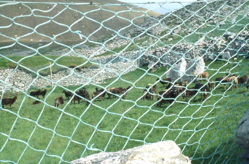
169 Soay sheep, Ovis aries

170 St. Kilda

171 Behaviour of the total population size over time The total population of Soay sheep, Ovis aries on St. Kilda is well known for reflecting large population crashes, when there is high mortality due to a combination of factors such as severe winter and high population density.

172 Classical model for female sheep An early model, resulting from likelihood-ratio tests between a small number of selected models is: 1 (P+M+h), 2 (M), 3:7 (M), 8+ (P+M) where P denotes population size, M denotes March rain and h denotes horn type. Regressions are logistic, and those on M are parallel. Note the use of age-classes. More detailed models result from Bayesian inference.

173 Individual covariates Age (use of age-classes) Sex (separate analyses: here only females) Climate Food Density Breeding history Size Health

174 Illustration of individual covariates

175 The likelihood for life-history data For general life-history data, the likelihood has the form below: where c is the time an individual was first captured, k is the time the animal was last known to be alive, d indicates the known death of the animal (1 or 0), w is an indicator variable for being seen occasion, and is a probability that an animal is never seen after an occasion, when it was known to be alive.

176 Time-varying individual covariates Important individual covariates often vary with time, and contain missing values. One approach is to use models to impute missing values. Done by Bonner and Schwarz (Biometrics, 2006). Another is to construct the likelihood conditionally.

177 Dealing with missing values Consider now the case history: ( ). The traditional likelihood contribution is: 1 (1-p 1 ) 2 p 2 3 p 3 4 Forming the likelihood in stages, we write: 1 (1,0) 2 (0,1) 3 (1,1) 4 (1,0) 5 (0,0) and to accommodate missing values, we may write: 1 (1,0) 3 (1,1) 4 (1,0), in contrast to the traditional approach, in which this case history is omitted: a complete case analysis.

178 Age classes For Soay sheep we identify 4 age-classes for survival. These correspond to animals of years of life: 1, 2, 3-7, >7 We use these age-classes in the data summary table that follows.

179 Trinomial data for Soay sheep Year

180 Comparison: current weight vs birth weight Comparison of estimates of weight coefficients Trinomial with W Trinomial with B Lamb 0.88(0.16) 0.91(0.17) Yearling 0.28(0.09) -0.05(0.29) Adult 0.20(0.07) 0.60(0.25)

181 Goodness-of-fit

182 Classical model for female sheep A classical model, resulting from likelihood-ratio tests between a small number of selected models is: 1 (P+M+h), 2 (M), 3:7 (M), 8+ (P+M) where P denotes population size, M denotes March rain and h denotes horn type. Regressions are logistic, and those on M are parallel.

183 Soay sheep (Ovis aries) Search for age-classes with constant survival- Bayesian approach obtains finer/better categorisation, and more detailed description of survival in terms of covariates.

184 Age-dependence (females): Bayes Age-structure Posterior probability 1 ; 2:4 ; 5:7 ; ; 2:7 ; 8+ 1 ; 2:4 ; 5:7 ; 7 ; ; 2:3 ; 4:7 ; Note that with probability 1, lambs have a distinct survival rate. Often, the models with most posterior support are close neighbours of each other.

185 The Bayes solution is richer Cov >9 c h b N P M T A RE

186 References

187 SECTION 6 PARAMETER REDUNDANCY

188 Determining the parameter redundancy of non-linear models Collaborators: Ted Catchpole, Diana Cole

189 Outline Introduction and motivation Definitions; general rules Use of symbolic algebra; expansion theorems The PLUR decomposition; exhaustive summaries; reparameterisation; identifiability; weak identifiability Future work

190 Complex models and their parameters Compartment models Ecology Econometrics Hidden Markov models

191 Compartment models

192 Econometrics Identifiability of the simultaneous equation model: By t + x t = u t, where y t and u t are vectors of random variables, x t is a vector of non-random exogenous variables, B and are matrices of parameters, and u t has a normal distribution, with dispersion matrix. The parameter space is [B,, ], some of which may be constrained.

193 A simple naïve Bayesian network

194 Ecology Estimation of the annual survival probabilities of wild animals. Collect data on previously marked animals. These are either found dead or alive. Form probability models. Fit to data using maximum likelihood, or Bayesian methods.

195 Complexity Models may be complicated, incorporating age, cohort and time components. Models may be simplified by the use of covariates. Modern focus on multi-site data can produce models with many parameters. It is often unclear how many parameters can be estimated.

196 An example of a multi-site system Multisite Systems S AA A S AB BA S B S BB CA S AC S C CB S BC S The parameter S represents the transition, i.e. it represents both survival and movement CC S

197 The British heron census, Ardea cinerea

198 Climatic covariates: number of frostdays in Central England.

199 The Cormack-Jolly-Seber (CJS) model (1965) Consider a simple case in which all animals are adults, sharing a common probability of annual survival,. If p denotes the probability of recapture then the multinomial probabilities corresponding to any cohort, of known size, of marked birds have the form: p, 2 p(1-p), 3 p (1-p) 2, Parameters may be time-dependent appropriate for adult animals.

200 Illustration of CJS recapture probabilities: a 3-year study 1 p (1-p 2 )p (1-p 2 )(1-p 3 )p 4 2 p (1-p 3 )p 4 3 p 4

201 CJS recapture probabilities: what we can estimate 1 p (1-p 2 )p (1-p 2 )(1-p 3 )p 4 2 p (1-p 3 )p 4 3 p 4

202 Parameter redundancy This model has deficiency of one: we can only estimate the product, 3 p 4. All the other parameters can be estimated.

203 Parameter redundancy This model has deficiency of one: we can only estimate the product, 3 p 4. All the other parameters can be estimated. What if we only have two years of ringing?

204 Illustration of CJS recapture probabilities: a 3-year study + 2 cohorts 1 p (1-p 2 )p (1-p 2 )(1-p 3 )p 4 2 p (1-p 3 )p 4

205 References Bellman and Åström, (1970), Mathematical Biosciences. Goodman, (1974), Biometrika. Rothenberg, (197), Econometrica. Walter, (1982), Identifiability of state space models.

206 Section Introduction and motivation Definitions; general rules Use of symbolic algebra; expansion theorems The PLUR decomposition; exhaustive summaries; reparameterisation; identifiability; weak identifiability Future work

207 Parameter redundancy and identifiability A model is identifiable if no two values of the parameters give the same probability distribution for the data. A model is locally identifiable if there is a distance > 0, such that any two parameter values that give the same distribution must be separated by at least. A parameter redundant model has parameters that cannot be estimated. A parameter redundant model is not locally identifiable. Full rank models are essentially or conditionally full rank. An essentially full rank model is locally identifiable. Are essentially full rank models identifiable?

208 General rules In some cases it is possible to establish general rules for models of particular structures. This avoids having to use Maple (see later). A particular illustration of this occurs with age-dependent recovery models

209 Model notation for recovery models Ring-recovery models are described as, for example: C/A/C, T/A/C, T/A/T, C/C/T. In this notation, each model is specified by 3 letters, which designate, in order, 1. The way we model first-year survival: C or T; 2. The way we model adult survival: C, A or T; and A can have categories. 3. The way we model the recovery probability: C, A or T.

210 Steps: age-dependence also in. Consider, for example, the model denoted by C/A(2,2,3)/A(2,1,1,4). What can we estimate here? Here we have the parameters: 1, 2, 2, 3, 3, 4, 4, 4 1, 1, 2, 3, 4, 4, 4, 4

211 Steps: age-dependence also in. Consider, for example, the model denoted by C/A(2,2,3)/A(2,1,1,4). What can we estimate here? Here we have a single step, as shown: 1, 2, 2 3, 3, 4, 4, 4 1, 1, 2 3, 4, 4, 4, 4

212 Theorem 1 Suppose the first step occurs at age n, and let m be the number of parameters used in the first n years. If m = n+1, the model is parameter redundant. If 1 < m < n+1, then the step does not cause parameter redundancy. Furthermore, to test for parameter redundancy, the parameters occurring in the first n years can be discarded, and the count started anew in year n+1.

213 Theorem 2 In the age-dependent model T/A/A The step at age 1 year does not cause parameter-redundancy To determine any possible redundancy caused by a subsequent step, the age and parameter counts begin again after age 1 year, as in Theorem 1.

214 Section Introduction and motivation Definitions; general rules Use of symbolic algebra and expansion theorems The PLUR decomposition; exhaustive summaries; reparameterisation; identifiability; weak identifiability Future work

215 How to test for parameter redundancy in general Form an appropriate derivative matrix, D. Use Maple to determine the symbolic row rank of D. Use this to determine if the model if parameter redundant or full rank. We can also determine which parameter combinations can be estimated, if the model is parameter redundant.

216 The method The approach was for exponential family models. It is performed using a symbolic algebra package such as Maple. j 1. Calculate D = ( is the mean, are parameters). i 2. The number of estimable parameters = rank(d). 3. Solve T D = 0. The location of the zeros in indicates which are the estimable parameters. p f 4. Solve ij 0 to find the full set of estimable i1 i parameters; (j is the index for >1 solution to T D = 0).

217 Example 1: Cormack-Jolly-Seber Model Little Penguins, Eudyptula minor, capture recapture data (1994 to 1997) i probability a penguin survives from occasion i to i+1 p i probability a penguin is recaptured on occasion i The set of parameters is: = [ 1, 2, 3, p 2, p 3, p 4 ] etc p p p p p p p p p p p p P N

218 Forming the derivative matrix (take logs first) rank(d) = 5 < 6, so the model is parameter redundant. In order to see which of the original parameters we can estimate: Set T D = 0 T = [ 0, 0, - 3 / p 4, 0, 0, 1] Solving PDE, we find that the estimable parameters are: 1, 2, p 2, p 3, 3 p 4 ln(p) D p p p p p p p p p p

219 Expansion theorems These give conditions that ensure that results which hold for a particular configuration also hold for larger configurations. For instance, the CJS model always has deficiency one.

220 Example Cormack-Jolly-Seber Model with covariates We now set i = 1/{1+exp( a + bx i )} For example, x i could be the mean annual banding weight, or the SOI. = [a, b, p 2, p 3, p 4 ], and we find that the model is now full rank.

221 References Bekker et al (1994) Identification, equivalent models and computer algebra. Catchpole, Freeman and Morgan, (1996), JRSS B. Catchpole and Morgan, (1997), Biometrika Catchpole, Morgan and Freeman, (1998), Biometrika. Catchpole and Morgan, (2001), Biometrika. Cole and Morgan, (2009), Parameter redundancy with covariates. submitted.

222 Section Introduction and motivation Definitions; general rules Use of symbolic algebra; expansion theorems The PLUR decomposition; exhaustive summaries; reparameterisation; identifiability; weak identifiability Future work

223 Use of the PLUR decomposition If parameter redundant: Solve T D = 0. Zeros in indicate estimable parameters. Solve p i1 ij f i 0 to find full set of estimable parameters. If full rank: Determine whether essential () or conditionally () full rank using the PLUR decomposition. D = PLUR. If det(u) = 0, model is parameter redundant. If det(u) is close to 0 model is near parameter redundant.

224 Components of the PLUR decomposition, available in Maple We have D=PLUR. P is a permutation matrix, L is lower triangular, with 1s on the diagonal, U is upper triangular, R is reduced echelon form.

225 Use of the PLUR decomposition: penguin covariates We have D=PLUR. We find that ( x1 x2)(1 p Det( U) 1 exp( a bx ) exp( a bx ) 1 exp( a bx ) ) p 3 p 4 exp( a bx 2 1 )exp( a bx 2 ) 3 Hence the model is full rank only if x 1 x 2, irrespective of x 3.

226 Example 2: Near-singular model Consider the model with parameter set, [ 1,1, 1,2, 1,3, a, 1, a ] This is a T/C/A(1,1) recovery model. It is full rank, but from the PLUR decomposition, we find, irrespective of 1,3

227 A complete theory? Maple (eg) can provide all the answers: Form the derivative matrix Find its rank Solve the Lagrange equations (parameter redundant) Form the PLUR decomposition (full rank) However it can run out of memory if used routinely for complex problems. Numerical procedures may then be used. The symbolic approach may still follow from identifying exhaustive summaries and reduced form exhaustive summaries

228 CJS model: removal of a cell 1 p (1-p 2 )p (1-p 2 )(1-p 3 )p 4 2 p (1-p 3 )p 4 3 p 4 The set of cells here has a redundancy.

229 Examples of exhaustive summaries We see from the last slide that we may simplify the formation of the derivative matrix by identifying a sufficient set of means. In fact we have already been doing that, by not using the last cell in each multinomial, from each row. Note the effect of missing data. These may affect rank.

230 Recapture of Dippers, Cinclus cinclus The table shows capture-recapture data for European Dippers in

231 Example 3 Tag Returns Fisheries Model Jiang et al (2007): Striped Bass, Morone saxatilis. = [ F, M 1, M 2, M 3, C 1, C 2, C 3, ], F instantaneous fishing mortality rate M a instantaneous natural mortality rate, at age a C a selectivity coefficient for age a (a > 3 C a = 1) reporting probability P ijk probability fish tagged at age k, released year i harvested and returned year j P ijk j1 exp vi F C M 1 exp F C M kvi kvi k ji k ji FC FC k ji k ji M k ji

232 Reparameterisation

233 Reparameterisation to produce a structurally simpler Q

234 Conclusions from the fisheries example In this example Maple lacks memory. In this example we move from 16 to 24 parameters. We find a deficiency of 8 in the new parameter space. Thus the model is full rank. Note that Jiang et al., used numerical analysis and found a deficiency of 9, as the model is nearsingular (revealed by a PLUR decomposition in the new parameterisation).

235 Example 4: a multi-state example

236 Reparameterisation example Form a set of sufficient means from the non-zero elements of the. Form an exhaustive summary from the non-zero elements of the component matrices. The result is 14 parameter combinations. Resulting derivative matrix has rank 12. Determine the reduced form exhaustive summary from solving the Lagrange partial differential equations. Use extension theorem. Previously (Hunter and Caswell, 2008) a numerical approach has been used.

237 Section Introduction and motivation Definitions; general rules Use of symbolic algebra; expansion theorems The PLUR decomposition; exhaustive summaries; reparameterisation; identifiability; weak identifiability Future work

238 Weak identifiability: the Bayesian context A parameter is said to be weakly identifiable when ( Y) ¼ p(). This is the counterpart to near-redundancy. For each parameter in a model, Garrett and Zeger(2000) considered the overlap of prior and posterior. Form = s min(p(), ( Y))d. Garrett and Zeger suggest ad-hoc threshold of = This works well for ecological applications.

239 Recapture of Dippers, Cinclus cinclus The table shows capture-recapture data for European Dippers in

240 A Bayesian perspective: the CJS model In population ecology we may devise models with parameters that cannot be estimated from the data Symbolic algebra can be used to examine whether a model is parameterredundant In a Bayesian context, it is interesting to consider the overlap between priors, p() and posteriors ( x) p p p p5 p6 p7

241 Male mallard, Anas platyrhyncos , , , , , a 1, , , , a Model: T/C/A (1,1) 1,i, a, 1, a here only two parameters, a and a are strongly identified. The model is nearredundant.

242 Relationship of overlap to interquartile range: simpler to calculate

243 Other areas Econometrics (Rothenburg) Compartment modelling (Walter) Contingency tables (Goodman) Naïve Bayesian Networks (Whiley)

244 A simple naïve Bayesian network

245 Naïve Bayesian Networks in general We have n observable nodes, Y 1,, Y n, and a single observable node Z. All nodes are binary. 2n+1 parameters: p, 1 1,, n 1 1 0, n 0.

246 Naïve Bayesian network ctd In this example we can use a reparameterisation to show that For n>2 the model is full rank We can use the PLUR decomposition to determine parameter redundant sub-models: for example, when n=3, Det(U)=-p 3 (1-p) 3 ( ) 2 ( ) 2 ( ) 2. Previously conclusions followed a particular analysis.

247 Compartment models

248 Simple compartment model

249 Conclusion: new work Use of covariates Use of exhaustive summaries Use of PLUR decomposition Conclusions for complex examples using the same approach Overlap of priors and posterior

250 Acknowledgement The work of Diana Cole was supported by the EPSRC grant for the NCSE.

251 References Cole, D.J., Morgan, B.J.T. and Titterington, D. M. (2010) Determining the parametric structure of models, Mathematical Biosciences. Cole, D.J. and Morgan, B.J.T. (2010) Parameter redundancy with covariates, Biometrika. Garrett and Zeger, (2000), Biometrics. Gimenez et al., (2003), Biometrical J. Gimenez, Morgan and Brooks, (2008), J. Env. and Ecol. Stats. Hunter and Caswell, (2008), J. Env. and Ecol Stats. Jiang et al., (2007), JABES. Whiley, (1999), Glasgow PhD thesis.

252 SECTION 7 STATE-SPACE MODELLING

253 References

254 Information about wildlife systems Diverse sources of data often exist: Demographic studies Population surveys (censuses) Trends in demographic processes (survival, productivity) and abundance are often investigated separately. But abundance and demography are related Combined estimation is appealing

255 Questions How do we form models and likelihoods for the different sources of data? How do we combine likelihoods? Do we have to form exact likelihoods? Why not take estimates from some likelihoods and plug them into other likelihoods?

256 Fecundity The key demographic processes involve survival, reproduction and movement. Estimation of fecundity can be challenging, but is typically easier than the estimation of survival. For example, Cory s shearwaters (Calonectis diomedea) lay just one egg.

257 Population surveys We obtain information on abundance from population surveys Typically the surveys are annual and the end-result is a single number summarising abundance: number of breeders at time t total number of animals The numbers are either estimates or indices of the actual numbers Populations exhibit a range of dynamics Compare dynamics of linnets, lapwings, herons and Soay sheep

258

259 Dynamics

260 Modelling survey data I There are, potentially, several aims in modelling survey data: To estimate true population size; To estimate biologically relevant parameters; To predict future population sizes. We shall provide an all-purpose method The first task is to build a model for all variables, observable or not

261 Modelling survey data II Abundance and demography are related: Abundance at time t is a function of survival, fecundity and abundance at time t-1. A state-space model framework is often used to make this idea explicit.

262 State-space models I A state-space model consists of 2 stochastic parts: 1. A dynamic model describing the evolution of a state from one year to the next: n t1 T n t t t 2. A model linking the observations to the state : y t Z t n t t The terms ε t and η t are errors incorporating: ε: process variability η: measurement uncertainty

263 State-space models II State-space models can be recognised as stochastic versions of But they are much more general (e.g. non-linear etc)

264 General definition A state-space model consists of two stochastic processes: An unobserved state process, n t, that is a function of past values, n t-1 State process density: g(n t n t-1 ;θ). A known observation process, y t, that is a function of the current state Observation process density: f(y t n t ;θ). θ: system parameters Could be time and space-dependent

265 Inference for state-space models Inference problems for state-space models fall into three broad categories: 1. Filtering: p(n t y 1:t ) 2. Smoothing: p(n t y 1:T ) 3. Prediction: p(n t+m y 1:t ), m>0.

266 Inference for state-space models Inference problems for state-space models fall into three broad categories: 1. Filtering: p(n t y 1:t ) 2. Smoothing: p(n t y 1:T ) 3. Prediction: p(n t+m y 1:t ), m>0. Filtering is the key problem, since it forms the basis of everything else In general, it involves evaluating high-dimensional integrals, which can be problematic. But see...modelling Population Dynamics Workshop (Andrew Thomas)

267 Linear Gaussian model A special case is the linear Gaussian model: n y t Ttnt ~ N0, Q 1 t t t t Z n n t : numbers at age t T t : Leslie matrix Y t : observed abundances θ includes survival, fecundity etc t t t ~ N n 0, H t 1 ~ N a1, t P 1 In this case, the Kalman algorithms can be used to estimate n t and θ No need for numerical or stochastic integration Details in Besbeas et al (2002).

268 The Kalman filter (KF) The following equations constitute the KF (Durbin and Koopman, 2001): with and. The algorithm can be derived and expressed in several ways. t t t t t t t t t t t t t t T a a v M F a a Z a y v 1 1 t t t t t t t t t t t t t t t t t t t t Q T T P P M M F P P P Z M H Z P Z F 1 1 t,t, 1 1 n 1 E a 1 n 1 P Cov

269 Related algorithms Missing values, prediction, smoothing follow from basic output: Missing values/prediction Use of a t+1 Natural extension to m-steps Smoothed estimates Result from a t t and another set of explicit recursions

270 The likelihood function The likelihood function also follows from basic output: logl kf 1 1 constant log F vf v 2 t t t t The parameters θ include demographic parameters, f from the matrix population model.

271 Combining likelihoods Assuming independence, we integrate the demographic and survey information on θ into a joint likelihood: L j,, p, f, L,, pl, f, mrr kf

272 Mark recapture recovery data Census data L mrr,,p Integrated Population Modelling Combining Sources of Information L kf,f, L mrr j,, p, f,,, pl, f, L kf

273 Advantages of integration 1. Simultaneous description of all the data 2. Generally more precise parameter estimators 3. Reduction in the correlation of estimators arising from census data alone 4. Coherent estimation of parameters not estimable from separate analyses

274 Example I: Lapwings (Besbeas et al, 2002) The Lapwing in Britain has been declining for several years. Amber list of species of conservation concern in Britain. Regarded as an indicator species for farmland birds.

275 Lapwing ring-recovery data Data on Lapwings ringed as chicks during the years Year Ringed Number Ringed Year Recovered

276 Lapwing survey data Use an index based on the Common Birds Census. Annual territory counts are made at a number of survey sites, and from these an index is estimated from a generalized linear model. Lapwing index is available from 1965 to Year Population Size

277 SSM: Observation model Let N 1,t denote the true number of one-year old female birds at time t, and N a,t denote the number of adult female birds at time t. We assume that y t N N a, t, ~ 2 where 2 is essentially an estimation error. We then impose a process model on the underlying population sizes

278 SSM: Process model A natural model will be to assume that N, ~ a t Bin N1, t1 Na, t1, a, t1 and N Po N ~ 1, t a, t1 t1 1, t1 f Here f t denotes the productivity rate (number of females per female) These can be easily and accurately approximated by Normal distributions, even for small population sizes.

279 Normal SSM with t a t a a a t a N N f N N t t a t N N y a a a t t a t a t t N N Var f N Var 1 1, 1 1,, 1 1, 1, 2 t Var

280 Parameter Modelling We allow each of our parameters potentially to vary with time as follows: Survival: logit Φ 1,t = α 1 +β 1 fdays t logit Φ a,t = α 1 +β 1 fdays t Productivity & recovery: log f t = α ρ +β ρ t logit λ t = α λ +β λ t

281 Likelihoods and Integrated Model Component likelihoods: Mrr: Survey: L mrr Joint Likelihood:,, L 1 a kf,,, 1 a f Assuming mrr and census data are independent L j,, f, L,, L,,, 1, a mrr 1 a kf 1 a f

282 Lapwing results Model Φ 1 (fdays),φ a (fdays)/λ(year)/f(year)

283 Parameter estimates Estimate SE Parameter Mrr Joint Mrr Joint Φ 1 intercept Φ 1 slope Φ a intercept Φ a slope λ intercept λ slope f intercept f slope σ Minor differences between mrr and joint estimates/ses The original Poisson/binomial model provides very similar results but is more difficult to fit Integrated modelling allows estimation of productivity

284 Assumptions made Normal errors Linear state-space model Known Kalman filter starting values Dispersion properly ascribed Independence between different data sets Observation variance cannot depend on the current state(s)

285 How to initiate the filter Using prior information (when available) Otherwise Unconditional initialisation Diffuse initialisation Approximate diffuse Exact diffuse Maximum-likelihood Use of stable age-distribution

286 Using the stable age-distribution The initial mean vector a 1 is taken to be proportional to the stable age distribution, with a maximal positive CI, e.g. Practical issues with v: a1 v, P1 diag a , Unknown parameters is Leslie matrix, T Time-varying matrix model, T t. 1 Details in Besbeas and Morgan (2007a)

287 Pros and cons of the methods Unconditional initialisation: limited to stationary systems. Approximate diffuse initialisation: arbitrary decisions are required. Exact diffuse initialisation: difficult for complex models and multivariate observations. Maximum likelihood: Multiple and/or boundary optima. Use of stable age-distribution: simple, and uses the Leslie matrix. Best in simulation comparisons.

288 Approximate Integration Recall we maximise: L j,, f, L, L, f, mrr kf Calculation of L j difficult when L mrr is derived from specialised programs (e.g. MARK) or raw data not available. Simplify calculations using asymptotic distribution of MLEs: ˆ ~ N, ˆ replacing by. Equivalently, log L mrr ˆ ˆ 1 const 0.5 ˆ loglˆ ; ˆ, ˆ mrr

289 Comparison of Lmrr and Lˆ ; ˆ,ˆ mrr

290 Approximate Joint Likelihood Now maximise Lˆ j, f, Lˆ, ˆ, ˆ L, f, mrr kf Nuisance parameters in L mrr (e.g. ) omitted details in Besbeas et al (2003)

291 Lapwing Parameter Estimates Parameter Estimate Standard Error Exact Approximate Exact Approximate 1 intercept slope a intercept a slope intercept slope intercept slope

292

293 Multi-site state-space models Basic structure of the state space model is the same: n t1 T t n t t State vector, n t will now include site-specific states y t Z t Observations y t will now be multivariate as site-specific observations will be made at each time point. n t t

294 Multi-site mark recapture data Multi-site census data Integrated Population Modelling Combining Sources of Information,, f, L mrr,,p L kf L mrr L j,, p, f,,, pl,, f, kf

295 Advantages of MULTI-SITE integration 1. Simultaneous description of all the data 2. Generally more precise parameter estimators 3. Reduction in the correlation of estimators arising from census data alone 4. Coherent estimation of parameters not estimable from separate analyses

296 Simulation Ringed animals are located in two distinct geographical sites. The animals are marked at an initial time point and then on subsequent occasions the sites are revisited and any resightings of marked individuals are recorded and recoveries of dead marked animals are made. Suppose also that total census counts are made at each time period for each of the sites. The simulation is run for 5 periods of recapture 15 census counts.

297 Simulation Parameters arising from mark-recapture-recovery data: (r): annual survival probability at site r p(r): capture probability at site r : recovery probability (r,s): movement probability of an animal from site r to site s Standard Arnason-Schwarz Model

298 Simulation N J (x): Number of juvenile animals in site x N A (x): Number of adult animals in site x t t A A J J t A A J J N N N N f f f f N N N N (2) (1) (2) (1) (2,2) (2) (1,2) (1) (2,2) (2) (1,2) (1) (2,1) (2) (1,1) (1) (2,1) (2) (1,1) (1) (2,2) (2) (1,2) (1) 0 0 (2,1) (2) (1,1) (1) 0 0 (2) (1) (2) (1) t t A A J J t N N N N y y (2) (1) (2) (1)

299 Simulation Results Parameter Simulated Value MRR Data Only MRR and Census (1) (0.0999) (0.0798) (2) (0.1064) (0.0970) p(1) (0.1291) (0.1207) p(2) (0.1889) (0.1669) (1,2) (0.2101) (0.1153) (2,1) (0.1893) (0.1691) (0.1012) (0.1009) f (0.0714) (0.2089)

300 Example II: Cormorants (McCrea et al, 2010) Great Cormorant, Phalacrocorax carbo sinensis

301 Three neighbouring colonies: Vorsø (VO) Mågeøerne (MA) Stavns Fjord (SF)

302 Recapture data collected between 1989 and 1994 Initial ringing was carried out on non-breeding individuals Birds were not recaptured until they had become breeding individuals Must model transition between non-breeding and breeding states as well as geographical movements between the colonies

303 Multi-site Cormorant census data 6000 VO MA 6000 SF

304 Transitions

305 State and Observation Equations t B SF B MA B VO N SF N MA N VO t SF MA VO SF MA VO t SF MA VO SF MA VO B B B N N N B B B N N N t SF MA VO t SF MA VO SF MA VO t SF MA VO B B B N N N y y y

306 Model Selection Model n AIC AIC Á(from state + time); B(from to); N(to); R(from + T ); f(site); ¾( ) Á(from state + time); B(from); N(to); R(from + T ); f(site); ¾( ) Á(from state + time); B(to); N(to); R(from + T ); f(site); ¾( ) Á(from state + time); B(from); N(from to); R(from + T ); f(site); ¾( ) Á(from state + time); B( ); N(to); R(from + T ); f(site); ¾( ) Á(from state + time); B( ); N(from to); R(from + T ); f(site); ¾( ) Á(from state + time); B( ); N(to); R(from + T ); f( ); ¾( ) Á(from state + time); B( ); N(from to); R(from + T ); f( ); ¾( ) Á(from state + time); B( ); N(to); R(T ); f( ); ¾( ) Á(from state); B( ); N(to); R(from + T ); f( ); ¾( ) Á(from state); B( ); N(from to); R(T ); f( ); ¾( ) Á(from state); B( ); N(to); R(T ); f(site); ¾( ) Á(from state); B(from); N(to); R(T ); f( ); ¾( ) Á(from state); B(to); N(to); R(T ); f( ); ¾( ) Á(from state); B( ); N(to); R(T ); f( ); ¾( ) Á(from state); B( ); N(to); R(T ); f( ); ¾(site) Á(from state); B( ); N(to + time); R(T ); f( ); ¾( ) Á(from state); B(time); N(to); R(T ); f( ); ¾( )

307 Integrated Population Model Parameter Mark-recapture MLE (SE) Integrated MLE (SE) Á ( 0.31 ) 0.47 ( 0.26 ) Á ( 0.45 ) 1.48 ( 0.24 ) Á ( 0.28 ) 0.60 ( 0.15 ) Á ( 0.27 ) 1.18 ( 0.12 ) Á ( 0.30 ) 0.94 ( 0.16 ) Á ( 0.21 ) 0.91 ( 0.16 ) Á ( 0.36 ) 0.87 ( 0.16 ) Á ( 0.18 ) 0.39 ( 0.12 ) Á ( 0.20 ) 0.58 ( 0.15 )

308

309 References Besbeas et al (2002) Biometrics, 58: Besbeas et al (2003) JRSSC, 52: Besbeas and Morgan (2007) Submitted Besbeas and Morgan (2007a) Submitted Besbeas et al (2009) in Modelling Demographic processes in marked populations. Borysiewicz et al (2009) in Modelling Demographic processes in marked populations. Durbin and Koopman (2001) Time series analysis by state-space methods Gautier et al (2007) Ecology, 88: Harvey (1989) Forecasting, structural time series models and the Kalman filter. King et al (2007) JRSSC, 57: McCrea et al (2010) JABES, 15: Tavecchia et al (2009) American Naturalist, 173:

310 SECTION 8 BAYESIAN ANALYSIS

311 Bayesian Methods in Ecology Collaborators: Steve Brooks Ruth King Olivier Gimenez

312 Bayesian methods in ecology: Outline History and Introduction Bayes vs Classical Selecting a prior Bayesian Integration Bayesian p-values Model selection

313 History Bayesian methods date to the original paper by the Rev. Thomas Bayes which was read to the Royal Society in Known then as inverse probability the approach dominated statistical thinking throughout the 19 th Century.

314 What is the Bayesian Approach? The approach is based upon the idea that the experimenter begins with some prior beliefs about the system And then updates these beliefs on the basis of observed data This updating procedure is based upon what is known as Bayes Theorem: ( Data) / f(data ) p()

315 A Difference in Philosophy The Classical approach provides a quite distinct philosophy from the Bayesian one. Bayesians believe that the model parameters have a true but unknown distribution which is represented by. The Classical statistician believes that the model parameters have a true but unknown value, which is estimated by the MLE.

316 Summarising the Bayesian s Beliefs The posterior distribution or the corresponding marginal distributions are the best summaries of the data. However, point estimates and uncertainty intervals are often more interpretable. It is the process of summarising the posterior that is the source of the computational complexity of the Bayesian approach. The classical approach also requires computation, but the maximisation of the likelihood function is usually relatively straightforward.

317 Point Estimates Though there are various ways to obtain point estimates for parameters of interest from the posterior, the most common is to take the posterior mean. The posterior mean is obtained via integration: E () = s ( Data) d.

318 Integration Problems There are two problems with this integration: 1. For realistically complex problems the integration is not analytically tractable and numerical methods must be used. 2. Bayes theorem only gives us the posterior distribution up to a constant of proportionality. [Recall: ( Data) / f(data ) p()] Thus the normalisation constant must be determined before the mean can be computed

319 The Classical Interval The Classical interval is known as the confidence interval. Given data Y, the 100(1-)% confidence interval [a(y),b(y)] for then satisfies the statement: P([a(Y),b(Y)] contains ) = 1-. Since is assumed fixed, it is the interval (constructed from the data) that is uncertain - it s randomness derives from the stochastic nature of the data under theoretical replications of the data collection process.

320 The Bayesian Interval The Bayesian interval is known as the credible interval. Given data Y, the 100(1-)% credible interval [a,b] for then satisfies the statement: P ( lies in [a,b])= 1-. Here, it is that is the random variable and the interval is fixed - the Bayesian conditions on the data observed rather than thinking about the long-term properties of the estimation procedure under theoretical replications of the datacollection experiment. [Recall Classical interval: P([a(Y),b(Y)] contains ) = 1-.

321 The Benefits of Being Bayesian For Example: It s no longer necessary to restrict attention to normal models. More complex (integrated, state-space) processes can be analysed with little additional effort. Unrealistic assumptions and simplifications can be avoided. Random effects and missing values are easily dealt with. Model choice and model averaging are relatively easy even with large model spaces.

322 Prior Elicitation and Specification Before we go on to discuss further the computational tools that have fuelled the Bayesian Revolution we pause to think a little more deeply about the prior elicitation and specification process. There are basically two situations that can be encountered: There is no prior information There is prior information that needs to be expressed in the form of a suitable probability distribution.

323 Informative Priors These priors aim to reflect information available to the analyst that is gained independently of the data being studied. A prior elicitation process is often used which involves choosing a suitable family of prior distributions for each model parameter and then attempting to find parameters for that prior that accurately reflects the information available. This is often an iterative process.

324 Prior Elicitation The analyst might begin by getting some idea of the range of plausible model parameter values and using this to get suitable prior parameters. Plots can be made and summary statistics calculated which can then be shown to the expert to see if they are consistent with their beliefs. Any mismatches can be used to alter the prior parameters and the process is repeated.

325 No Information In the absence of any prior information on one or more model parameters we wish to ensure that this lack of knowledge is properly reflected in the prior. Typically, this is done by choosing a prior distribution with a suitably wide variance. At first, it may seem that taking a flat prior that assigns equal probability to all possible parameter values is a sensible approach.

326 Flat Priors However, flat priors are rarely invariant to reparameterisations of the model. What may appear flat for parameters under one parameterisation may be far from flat under another. In ecological applications where many parameters of interest are probabilities (e.g., survival, recapture etc.) expressed as logistic regressions e.g., logit( t ) = + t. Do you want a prior that is flat on -space or (, )-space?

327 Flat Priors ctd Another problem with flat priors is that for continuous variables, these are improper distributions unless bounds on the parameter space are imposed. Improper priors can lead to improper posteriors which, in turn, can mean that the posterior mean simply does not exist. On the other hand, the imposition of bounds which are too restrictive may mean an unrealistically restricted posterior is obtained.

328 Jeffreys Prior One solution is to use the Jeffreys prior. This prior attempts to minimise the amount of influence of the prior on the posterior and is invariant to reparameterisations of the model. It is based upon estimation of Fisher s Information matrix the same matrix used to estimate Classical SE s.

329 Vague Priors In practice most people choose vague priors which are both proper and have large variance. An alternative is to adopt a hierarchical prior structure in which the prior parameters are assumed unknown and themselves given hyperprior distributions. For example, rather than saying» N(0, 1000) We might instead say» N(0, 2 ), with 2» (a,b).

330 Vague Priors ctd This dilutes the influence on the posterior of any prior assumptions made and essentially creates random effects of the model parameters. We will explore the parallel between hierarchical priors and random effects later on. The influence of the prior can always be assessed via a sensitivity analysis and we will also return to this later.

331 A Simple Example Let s take a simple example to recap some of the main issues discussed so far. 120 deer were radio-tracked over Winter. Number released Alive Dead Other Treatment Control

332 Example ctd... So, n=57 deer were assigned to the treatment group of which m=19 survived the Winter, Of interest is the probability of over-winter survival, call it q, for the general population within the treatment area. The obvious estimate is simply to take the ratio m/n=19/57. How would the Classical statistician justify this estimate?

333 The Model and MLE Our model is that we have a simple Binomial experiment (assuming independent and identically distributed draws from the population), so that The classical approach is to maximise the corresponding likelihood with respect to q to obtain the entirely plausible MLE: q = m/n = 19/57.

334 The Bayesian Approach The Bayesian starts off with a prior. Now, the one thing we know about q is that is a continuous random variable and that it lies between zero and one. Thus, a suitable prior distribution might be the Beta which is defined on this range. Suppose we assume a priori that q» (a,b) So that

335 The Posterior Then, we have that i.e., q» (a+m, b+n-m) a posteriori. If we take a Uniform prior i.e., a=b=1, then we get the following prior and posterior distributions.

336 Posterior Plot

337 Posterior Summaries Similarly, under the Uniform prior we get: Posterior mean = Posterior mode = Posterior standard deviation = Recall that the MLE is with a standard error of

338 The Posterior ctd... For a general prior, the posterior has mean where w = n/(a+b+n). Thus, the posterior mean is a weighted average of the prior mean and the MLE. Note that as n increases, the weight w tends to 1 and so the posterior mean converges to the MLE.

339 More Posterior Plots

340 The Posterior ctd The posterior mean converges to the MLE irrespective of the prior parameters a and b (though the speed at which convergence occurs will vary with the prior). Similarly, the posterior variance converges to zero as the sample size increases. Thus, the posterior itself converges to a point mass at the MLE.

341 A General Result This is a general result, the Bayesian and Classical estimates will always agree if there is sufficient data, so long as the MLE is not explicitly ruled out by the prior.

342 Which parameters can we identify? In population ecology we may devise models with parameters that cannot be estimated from the data Symbolic algebra can be used to examine whether a model is parameterredundant In a Bayesian context, it is interesting to consider the overlap between priors, p() and posteriors ( x) p p p p5 p6 p7

343 Male mallard, Anas platyrhyncos , , , , , , , , ,9 Model: 1,i, a, 1, a here only two parameters, a and a are strongly identified a 1 a

344 Bayesian Integration Made Easy Recall that Bayesian inference is based upon the estimation of posterior summaries such as the mean. And that these require integration of the posterior density e.g. E () = s ( Data) d. Expectations of this sort can be estimated by drawing samples 1,, T from the posterior distribution and then calculating the sample mean. This is known as Monte Carlo Integration.

345 From Integration to Sampling Thus, we replace the integration problem by a sampling problem. Two problems: In general, ( Data) represents a highdimensional and complex distribution from which samples would usually be difficult to obtain. In addition, large sample sizes are often required and so powerful computers are needed to generate these samples.

346 The 1990 s At the beginning of the 1990 s two things happened: The computer revolution which made powerful computers an affordable reality. MCMC was introduced to the statistical literature which provided a framework for generating samples from arbitrarily complex distributions.

347 Markov Chain Monte Carlo MCMC methods perform Monte Carlo Integration using a Markov chain to generate observations from. A Markov chain is simply a stochastic sequence of numbers where each value in the sequence depends only upon the last. We might label the sequence 0, 1, 2, etc.

348 MCMC ctd The value for 0 is chosen from some arbitrary starting distribution. At time t, we update the state of the chain from t to t+1. This updating is performed in such a way that the probability distribution associated with the t th observation gets closer and closer to ( Data) as t increases. We say that the distribution of the chain converges to. We return to the concept of convergence later on.

349 MCMC Magic MCMC therefore allows us to construct a sequence of values whose distribution converges to the posterior distribution of interest. We can then use this sequence of values to obtain empirical (Monte Carlo) estimates of any posterior summaries of interest e.g., posterior means. The beauty of MCMC is that the updating procedure remains relatively simple no matter how complex the posterior distribution of interest.

350 Updating our Chain OK, so we can do the integration by sampling from the posterior. We can sample from the posterior by generating a Markov chain. We construct a Markov chain using an appropriate updating scheme. But how do we do these updates? There are several standard approaches

351 Metropolis Hastings Most MCMC methods are special cases of the general Metropolis Hastings scheme. The MH scheme generates t+1 from t in a two-step procedure. Step 1. At iteration t, sample» q( t ). is known as the candidate point q is known as the proposal distribution

352 MH ctd Step 2. With probability set t+1 = else, set t+1 = t (acceptance) (rejection) Steps 1 and 2 are then repeated to obtain first 1 and then 2 etc.

353 Flavours of MH Within the MH scheme there are a number of special cases depending upon the (essentially arbitrary) choice of proposal distribution. One basic and common choice is to base the proposal around the current point e.g.,» N( t, 2 ). In this case, the acceptance ratio simplifies so that ( t, ) = min [1, ()/( t )]

354 Tuning the RW Metropolis Algorithm This is known as the random walk Metropolis algorithm. In order to balance the size of the proposed moves with the chance of accepting them the proposal variance is often tuned to obtain an acceptance rate of 20-40%. Most MH algorithms require some initial pilot tuning in order to get satisfactory performance.

355 Why is the Size of the Move Important? If you propose extremely small jumps, you are bound to accept them, but you will take a long time to move around the state space. Small jumps induce correlations (known as autocorrelations) between successive observations. If you have strongly correlated observations, you require far bigger sample sizes and therefore longer MCMC runs.

356 Good Trace/Bad Trace Variance too small Just right Too large

357 Single-Update MH Typically, the posterior will be highdimensional. In this case, we can either update all parameters simultaneously. Or, we can update each parameter in turn. This is known as single-update Metropolis Hastings. Sometimes it is convenient to do something in between and update parameters in blocks.

358 Gibbs Updates A special case of the single-update MH algorithm arises if we set the proposal distribution for any parameter to be the conditional posterior distribution of that parameter given current value of the others. In this case, the acceptance probability is always exactly 1. This is known as a Gibbs-sampler (or simply Gibbs) update.

359 Gibbs Updates ctd One useful feature of the Gibbs update (beyond no longer having to perform the accept-reject step) is that it requires no pilot-tuning. Also the proposal is adaptive in that it depends upon the state of the other parameters and so changes from iteration to iteration. Gibbs updates tend to be highly efficient MCMC-wise but can be computationally more burdensome.

360 Hybrid Schemes In practice we often use a mixture of MH and Gibbs updates. For parameters with standard conditional distributions, we use Gibbs updates. And, for the rest, we might use random walk updates. Since Gibbs updates are so good, we would like to use them as often as possible

361 Conjugacy When selecting our prior, it is often useful to select what is known as a conjugate prior family. For a particular parameter, the associated prior is conjugate if the corresponding posterior conditional is of the same form. E.g., a Normal prior leading to a Normal posterior conditional. Conjugate priors are often adopted so that Gibbs updates can be used.

362 Posterior Summaries Posterior means and variances etc. are easily obtained. Intervals usually come in the form of Highest Posterior Density Intervals which are credible intervals with the minimum width. E.g., for a (1-)% HPDI, order the observations and take [ (i), (j) ] where i+j = T and T denotes the sample size.

363 Density Estimates Marginal density estimates are also often of interest. Basic histograms or kernel smoothed empirical estimates can be used. Rao-Blackwell estimates are also useful. Here, If the posterior conditional is standard, then the density estimate, f, is easily normalised.

364 Run Lengths There are two elements to be considered when determining the simulation length: The time required for convergence. The post-convergence sample size required for suitably small Monte Carlo errors. We begin with convergence assessment...

365 Convergence Assessment Here, we re looking to determine how long it takes for the Markov chain to converge to the target distribution. In practice, we discard observations from the start of the chain and just use observations from the chain once it has converged. The initial observations that we discard are referred to as the burn-in.

366 Trace Plots The simplest method to determine the length of the burn-in period is to look at trace plots. You can often see the individual parameters converging from their starting position to values based around a constant mean. This is a fairly efficient method, but is not robust.

367 Trace Plot Example Converged after, say, 2000 iterations?

368 Multiple Replications Running several replications from different starting points provides additional reassurance. Basically, if you run the chain several times from different starting points and they all give you the same posterior estimates... Then, this suggests that no major modes have been missed in any one simulation and that each has probably converged.

369 Convergence Assessment This approach is formalised in the so-called BGR diagnostic. Available in WinBUGS. There are various implementations, all based upon the idea of using an analysis of variance to determine whether or not there are any differences in estimates from different replications. The simplest implementation is to compare the width of the empirical 80%CI obtained from all chains combined, with the corresponding mean within-chain interval width. Convergence is assumed when these are roughly equal, implying that all chains have roughly equal variability i.e., similar amounts of information.

370 Prior Sensitivity As discussed earlier it is important to assess the sensitivity of key results to the prior assumptions. In the presence of reasonably informative data, there should be little prior sensitivity. Prior sensitivity in itself is not a problem, but... Extreme prior sensitivity often points to problems such as parameter redundancy or overly restrictive prior assumptions.

371 Bayesian P-values Bayesian p-values involve generating a new data set Y t from the model at each MCMC iteration. A discrepancy statistic D(Y t,e t ) is then used to measure the distance between the generated data and the corresponding expected values, e t. The proportion of times that D(Y,e t ) > D(Y t,e t ) is recorded and should be close to 0.5. Plots of D(Y,e t ) vs D(Y t,e t ) may also be useful.

372 Bayesian P-values Plot P-value here is 0.513

373 Model Selection In the classical framework, likelihood ratio tests or information criterion (e.g. AIC) are often used. There is a similar Bayesian statistic the DIC. This is programmed within WinBUGS however its implementation is not suitable for hierarchical models (e.g. random effect models). In addition, the DIC is known to give falacious results in even simple problems. Within the general Bayesian framework, there is a more natural way of dealing with the issue of model discrimination.

374 Bayesian Approach We treat the model itself to be a unknown parameter to be estimated. Then, applying Bayes Theorem we obtain the posterior distribution over both parameter and model space: ( m, m data) Ç L(data m, m) p( m ) p(m). Here m denotes the parameters in model m. Likelihood Prior on parameters in model m Prior on model m

375 Posterior Model Probabilities The Bayesian approach then allows us to quantitatively discriminate between competing models via posterior model probabilities: (m data) = s ( m, m data) d m Ç p(m) s L(data m, m) p( m ) d m Note that we need to specify priors on both the parameters and now also on the models themselves. Thus we need to specify a prior probability for each model to be considered.

376 Bayes Factors These are often used to compare models and are simply defined to be the ratio of the posterior odds to prior odds. For two models, m 1 and m 2, the Bayes factor of model 1 to model 2 is given by: BF 12 = (m 1 data)/p(m 1 ) (m 2 data) p(m 2 ) Kass and Raftery (1995) give the following rule of thumb guide: Bayes factor < > 150 Interpretation Not worth mentioning Positive evidence Strong evidence Very strong evidence

377 Model Averaging Model averaging obtains an estimate of a parameter, based on all plausible models, and takes into account both model and parameter uncertainty. For parameter, common to models m 1, m k, the model averaged estimate is: ( data) = (, m i data) k i=1 k = ( data, m i ) (m i data). i=1 Thus each estimate of is weighted according to the corresponding posterior probability.

378 Monte Carlo estimates The posterior probability of model m is given by: (m data) Ç p(m) s L(data m, m) p( m ) d m However E p [f(x)] = s f(x) p(x) dx. So that, (m data) Ç p(m) E p [L(data m, m)]. Thus, we can estimate this expression by using a Monte Carlo estimate.

379 Monte Carlo estimates ctd. The simplest approach is to draw observations 1, N from the prior distribution p(), and estimate, N L(data m) = N -1 L(data i, m) i=1! E p [L(data m, m)] as N! 1 Thus, this estimate converges to the posterior model probability (up to proportionality). Posterior model probabilities can be estimated by calculating this for each model and renormalising (so that the probabilities sum to one).

380 Further Monte Carlo estimates However, this approach is often very inefficient, and can be very unstable. Alternative approaches essentially involve changing the distribution from which the are drawn (and hence the expression for the Monte Carlo estimate). For example, an alternative estimate would be to sample from the posterior distribution and use, N L(data m) = [N -1 L(data i, m) -1 ] -1 i=1

381 General Comments The Monte Carlo estimates are the easiest to program and conceptualise. However, they are often very inefficient and do not always converge within a feasible number of iterations. In addition, each individual model needs to be considered in turn, which may be infeasible when there are a large number of models. We consider in more detail alternatives which use the same underlying principle as MCMC.

382 MCMC-based estimates We have a posterior distribution (over parameter and model space) defined up to proportionality: ( m, m data) Ç L(data m, m) p( m m) p(m) If we can sample from this posterior distribution then we are able to obtain posterior estimates of summary statistics of interest. In particular the posterior model probabilities can be estimated as the proportion of time that the chain is in each model. So, all we need to do is define how we construct such a Markov chain.

383 Reversible Jump MCMC The reversible jump MCMC algorithm allows us to construct a Markov chain with stationary distribution equal to the posterior distribution. It is simply an extension of the Metropolis- Hastings algorithm that allows moves between different dimensions. This algorithm is needed because the number of parameters, m, in model m, may differ between models. Note that this algorithm needs only one Markov chain irrespective of the number of models!!

384 Markov chain Each iteration of the Markov chain essentially involves two steps: 1. Within model moves updating each parameter using standard MCMC moves (Gibbs sampler, Metropolis-Hastings) 2. Between model moves updating the model using a reversible jump type move. Then, standard MCMC-type processes apply, such as using an appropriate burn-in, obtaining summary statistics of interest etc.

385 Within model moves: MH algorithm Recall, the MH algorithm involves two steps: 1. At each iteration k, with current parameter values k, sample a candidate point from some proposal distribution q, i.e. ~ q( k ). 2. Accept the proposed value with probability, min(1,a), where, A = and set k+1 =. ( data) q( k ) ( k data) q( k ) Else, if the move is rejected, set k+1 = k.

386 Between model moves: RJ step This is simply a generalisation of the MH algorithm, which allows moves between different models. A single move involves two steps: 1. Proposing to move to a different model; 2. Accepting this proposed model with some probability. To illustrate the RJ algorithm, we consider a particular example relating to variable selection (e.g. covariate analysis).

387 Example: variable selection Suppose that the survival rate is logistically regressed on possible covariates x and y. However, it is unknown a priori which covariates (if any) affect the survival rates. There are two possible models: 1. logit = + x; 2. logit = + x + y where and (and for model 2) are parameters to be estimated.

388 RJ update Suppose that the Markov chain is currently in model 1 (logit = + x). Step 1: Proposing new model. Set = (, ). Suppose that at iteration k of the Markov chain we are in state (, m) k. We propose to move to state (, m ), where = (,, ). Then, we simulate parameter value from some proposal distribution q.

389 RJ Update (cont) Step 2: Accept/reject step: Accept the new model m, and set (, m) k+1 = (, m ) with probability min(1,a), where, A = (,m data) P(m m ) (, m data) P(m m) q(), where P(m m ) denotes the probability of proposing to move from model m to model m. Else reject the move and set (, m) k+1 = (, m) k. Then, in the reverse move, where we propose to move from (, m ) to state (, m), we remove parameter (or equivalently set it equal to zero). This move is then accepted with probability, min(1,a - 1 ).

390 **General RJ updates** The previous RJ step can only be applied to nested models more generally, moves are possible between any two models: Step 1: Proposing new model. Suppose that at iteration k the Markov chain is in model m with parameters (, m) k. We propose to move to state (, m ). Then, we define a (bijective) function g, such that, (, u ) = g(, u) where u and u are sets of random variables with density function q(u) and q (u ), respectively.

391 **General RJ updates (cont)** Step 2: Accept/reject step: Accept the new model m, and set (, m) k+1 = (, m ) with probability min(1,a), where, A = (,m data) P(m m ) q (u ) (, u ) (, m data) P(m m) q(u) (, u) where P(m m ) denotes the probability of proposing to move from model m to model m. Else reject the move and set (, m) k+1 = (, m) k. This final term is called the Jacobian. This formula is not as complicated as it appears!!

392 Case Study: Soay sheep Heterogeneity within a population can often be explained via different covariates. For illustration we shall consider in detail MRR (mark-recapturerecovery) data relating to Soay sheep. Covariate values Capture history Missing values

393 Soay sheep We place vague priors on the parameters present in each model. Priors also need to be specified on the models. Placing an equal prior on each model places a high prior mass on models with a large number of age groups, since the number of models increases with the number of age groups. Thus, we specify we an equal prior probability on each marginal age structure and a flat prior over the covariate dependence given the age structure

394 Results Soay sheep We use the RJ algorithm to explore and summarise the posterior distribution. The posterior distribution is very complex, and so we present results from the marginal distributions for the survival rates only. We initially consider the age-dependence structure before the covariate dependence.

395 Age-dependence (females) Age-structure Posterior probability 1 ; 2:4 ; 5:7 ; ; 2:7 ; 8+ 1 ; 2:4 ; 5:7 ; 7 ; ; 2:3 ; 4:7 ; Note that with probability 1, lambs have a distinct survival rate. Often, the models with most posterior support are close neighbours of each other.

396 Covariate Dependence BF = 20 BF = 3 BF = Bayes factor

397 Influence of parameters Birth weight NAO Index Age 1 Age 10+

398 Results Shags (MRR data) Survival rate Recapture rates Recovery rate Posterior probability 1 (t), 2,3, A (t) p 1, p 2, p 3 (t), p A (t) 1, 2,3, A (t), 2,3, A p 1, p 2, p 3 (t), p A (t) 1, 2,3, A (t), 2, 3,A p 1, p 2, p 3 (t), p A (t) 1,3, 2, A (t), 2, 3, A (t) p 1, p 2, p 3 (t), p A (t) 1, 2,3, A Some variability but neighbouring models This model for the recapture rates has posterior probability

399 General Comments RJMCMC is the most widely used algorithm when there is model uncertainty. The acceptance probabilities for RJ moves are typically lower than for MH updates. Longer simulations are generally needed to explore both parameter and model space. Only a single Markov chain is necessary, irrespective of the number of possible models!! However, RJMCMC cannot (currently) be generally programmed in WinBUGS and specific codes generally need to be written.

400 The benefits of a Bayesian approach Random effects are easily incorporated Missing values are easily dealt with Hierarchical models are easy to construct Model averaging is easily done State-space models can be constructed without the need for normal approximations Easy application to longitudinal models Easy application of complex spline regressions.

401 Are there dangers in Bayesian methods? The main danger is that they will be used automatically. In the application of Bayesian methods, you first need to assign some basic probabilities (and perhaps utilities) to give the problem structure; then the computer can derive other probabilities. One must think about the basic values and it is not usually satisfactory to use a normal density and non-informative priors. This distinction between the thinking you and the un-thinking, calculating personal computer is essential. Dennis Lindley, Significance, 2004.

402 Possible reading Bayesian Model Averaging: a tutorial. (1999), Hoeting, J.A. et al. Statistical Science, 14, Model choice: A minimum posterior predictive loss approach. (1998) Gelfand, A.E. and Ghosh, S.K. Biometrika, 85, Bayesian model choice via Markov chain Monte Carlo methods. (1995) Carlin, B.P. and Chib, S. JRSSB, 57, Sensitivity of Bayes estimators to hyperparameters with an application to maximum yield from fisheries. (2004) Millar, R.B. Biometrics, 60,

403 The end