Experimental and Computational Studies on Cryogenic Turboexpander

Transcription

1 Experimental and Computational Studies on Cryogenic Turboexpander A Thesis Submitted for Award of the Degree of Doctor of Philosophy Subrata Kumar Ghosh Mechanical Engineering Department National Institute of Technology Rourkela

2 Dedicated to PARENTS

3 NATIONAL INSTITUTE OF TECHNOLOGY ROURKELA, INDIA Ranjit Kr Sahoo Professor Mechanical Engg. Department NIT Rourkela Sunil Kr Sarangi Director NIT Rourkela CERTIFICATE Date: July 9, 008 This is to certify that the thesis entitled Experimental and computational studies on Cryogenic Turboexpander, being submitted by Shri Subrata Kumar Ghosh, is a record of bona fide research carried out by him at Mechanical Engineering department, National Institute of Technology, Rourkela, under our guidance and supervision. The work incorporated in this thesis has not been, to the best of our knowledge, submitted to any other university or institute for the award of any degree or diploma. (Ranjit Kr Sahoo) (Sunil Kr Sarangi)

4 Acknowledgement I am extremely fortunate to be involved in an exciting and challenging research project like development of a high speed cryogenic turboexpander. It has enriched my life, giving me an opportunity to look at the horizon of technology with a wide view and to come in contact with people endowed with many superior qualities. I would like to express my deep sense of gratitude and respect to my supervisors Prof. S.K.Sarangi and Prof. R.K.Sahoo for their excellent guidance, suggestions and constructive criticism. I feel proud that I am one their doctoral students. The charming personality of Prof. Sarangi has been unified perfectly with knowledge that creates a permanent impression in my mind. I consider myself extremely lucky to be able to work under the guidance of such a dynamic personality. Whenever I faced any problem academic or otherwise, I ran to him, and he was always there, with his reassuring smile, to bail me out. I and my family members also remember the affectionate love and kind support extended by Madam Sarangi during our stay at Kharagpur and Rourkela. I also feel lucky to get Prof. R.K.Sahoo as one of my supervisors. His invaluable academic and family support and creative suggestions helped me a lot to complete the project successfully. I record my deepest gratitude to Madam Sahoo for family support all the times during our stay at Rourkela. I take this opportunity to express my heartfelt gratitude to the members of my doctoral scrutiny committee Prof. B. K. Nanda (HOD), Prof. A. K. Shatpaty of Mechanical Engineering Department, Prof. R. K. Singh of Chemical Engineering Department for thoughtful advice and useful discussions. I am thankful to my other teachers at the Mechanical Engineering Department for constant encouragement and support in pursuing the PhD work. I am indebted to the Cryogenic Division of Bhabha Atomic Research Centre (BARC), Mr. Tilok Singh and his Team for sharing their vast experience on turbine. I must confess had he not made arrangements for the experiments of our turbine in BARC, I would not be in a position to write these words now. I take this opportunity to express my heartfelt gratitude to all the staff members of Mechanical Engineering Department, NIT Rourkela for their valuable suggestions and timely support. I am deeply indebted to one of the project team members Mr. Biswanath Mukherjee for his cooperation and skilled technical support to complete the task in time. I record my appreciation for the help extended by Dr. Nagam Seshaiah during my research work. A friend in need is a friend indeed I have got a first hand proof of this proverb through the generosity of my friends and associates at NIT. Mr. Pradip Kumar Roy and Mr Suhrit iv

5 Mula, my good friends have been by my side all my life at NIT. I shall really miss the interesting and intellectually motivating company of my friends and colleagues. I am really grateful to my loving parents for their perseverance, encouragement with support of all kinds and their unconditional affection. With a smile on their faces but anxiety in their minds, they stood by my side in times of need. Their presence itself came as a soothing solace. I thank my stars to have such wonderful parents. My beloved wife had to undergo the rigours of my agony and ecstasy during the period of my research work. Sometimes she had to manage difficult and demanding situations all alone. I am sorry for this but feel proud of her. This thesis is a fruit of the fathomless love and affection of all the people around me my wife, parents, in-laws, grandparents, uncle and aunty, brother, my supervisors and my colleagues and friends. If there is anything in this work that is of value the credit goes entirely to them. (July 9, 008) (Subrata Kumar Ghosh) v

6 Abstract The expansion turbine constitutes the most critical component of a large number of cryogenic process plants air separation units, helium and hydrogen liquefiers, and low temperature refrigerators. A medium or large cryogenic system needs many components, compressor, heat exchanger, expansion turbine, instrumentation, vacuum vessel etc. At present most of these process plants operate at medium or low pressure due to its inherent advantages. A basic component which is essential for these processes is the turboexpander. The theory of small turboexpanders and their design method are not fully standardised. Although several companies around the world manufacture and sell turboexpanders, the technology is not available in open literature. To address to this problem, a modest attempt has been made at NIT, Rourkela to understand, standardise and document the design, fabrication and testing procedure of cryogenic turboexpanders. The research programme has two major objectives A clear understanding of the thermodynamic scenario though modelling, that will help in determination of blade profile, and prediction of its performance for a given speed and size. To build and record in open literature a complete turbine system. The work presented here can be broadly classified into seven parts. The first part is the genesis that builds up the problem and gives a comprehensive review of turboexpander literature. A detailed review of the development process, as well as all relevant technical issues, have been carried out and will be presented in the thesis. A streamlined design procedure, based on published works, has been developed and documented for all the components. Full details of the design process, from conception of the basic topology to production drawings are presented. A detailed procedure has also been given to determine the three-dimensional contours of the blades with a view to obtaining highest performance while satisfying manufacturing constraints. A cryogenic turboexpander is a precision equipment. Because it operates at high speed with clearances of 10 to 40 μm in the bearings, the rotor should be properly balanced. This demands micron scale manufacturing tolerance on the shaft and also on the impellers. Special attention has been paid to the material selection, tolerance analysis, fabrication and assembly of the turboexpander. An experimental set up has been built to study the performance of the turbine. The thesis presents the construction of the test rig, including the air / nitrogen handling system, gas bearing system, and instrumentation for measurement of temperature, pressure, rotational speed and vibration. Vibration and speed have been measured with a laser vibrometer. The prototype turbine has been successfully operated above 00,000 r/min. vi

7 The performance of a turbine system is expressed as a function of mass flow rate, pressure ratio and rotational speed. Based on the method suggested by Whitfield and Baines, a one-dimensional meanline procedure for estimating various losses and prediction of off design performance of an expansion turbine has been carried out. vii

8 Contents Certificate Acknowledgements Abstract Contents Nomenclature List of Figures List of Tables iii iv vi viii xi xv xx 1. Introduction 1.1. Role of Expansion Turbines in Cryogenic Processes Anatomy of an Expansion Turbine 1.3. Objectives of the Present Investigation Organization of the Thesis 5. Literature Review.1. A Historical Perspective 6.. Design of of Turboexpander 9.3. Assessment of Blade Profile Development of prototype Turboexpander 0.5. Experimental Performance Study 5.6. Off-Design Performance of Turboexpander 7 3. Design of Turboexpander 3.1. Fluid Parameters and layout of components Design of Turbine Wheel Design of Diffuser Design of Nozzle Design of Brake Compressor Design of shaft Design of Vaneless Space Selection of Bearings Supporting Structures 55 viii

9 4. Determination of Blade Profile 4.1. Introduction to Blade Profile Assumptions Input and Output Variables Governing Equations Results and Discussion Development of Prototype Turboexpander 5.1. Materials for the Turbine System Analysis of Design Tolerance Fabrication of Turboexpander Balancing of the Rotor Sequence of Assembly Precautions during Assembly and suggested Change Experimental Performance Study 6.1. Turboexpander Test Rig Selection of Equipment Instrumentation Measurement of Efficiency Experiment on Turboexpander with Aerostatic Bearings Experiment on Turboexpander with Complete Aerodynamic Bearings Results and Discussion Off Design Performance of Turboexpander 7.1 Introduction to Performance Analysis Loss Mechanisms in a Turboexpander Summary of Governing Equations Input and Output Variables Mathematical Model of Components Solution of Governing Equations Results and Discussion Epilogue 8.1 Concluding Remarks Scope for Future Work 156 ix

10 References 158 Appendices A. Production Drawings of Turboexpander B. Fabricated Parts of Turboexpander Curriculum Vitae x

11 Nomenclature A = cross sectional area normal to flow direction (m ) b = height (nozzle, wheel blade) (m) C = chord length (m) C r = absolute velocity of fluid stream (m/s) C 0 = spouting velocity (m/s) C P = specific heat at constant pressure (J/kg K) C s = velocity of sound (m/s) C 1 = integrating constant (dimensionless) C = integrating constant (dimensionless) D = diameter (wheel, brake compressor) (m) d = diameter (shaft) (m) DS = design speed rpm E = Young s modulus (N/m ) f = vibration frequency (Hz) h = enthalpy (J/kg) I = rothalpy (J/kg) k 1 = Pressure recovery factor (dimensionless) k = Temperature and Density recovery factor (dimensionless) K e = free parameter (dimensionless) K h = free parameter (dimensionless) K I = meridional velocity ratio (dimensionless) l = shaft length (m) L = length (m) LL = lower limit of tolerance (m) xi

12 M = Mach number (dimensionless) m = total number of difficulty factors (dimensionless) m = polytropic index (dimensionless) M N = Molecular weight of N kg/kmol m& = mass flow rate (kg/s) N = rotational speed (r/min) n = total number of dimensions in a loop (dimensionless) n s = specific speed (dimensionless) d s = specific diameter (dimensionless) P = power output of the turbine (W) p = pressure (N/m ) Q = volumetric flow rate (m 3 /s) R = Gas constant of the working fluid (J/kg.K) R = difficulty index for each tolerance (dimensionless) r = radius (m) r = radial coordinate (dimensionless) Re = machine Reynolds number (dimensionless) S = tangential vane spacing (m) s = entropy (J/kg.K) s = meridional streamlength (m) T = temperature (K) t = blade thickness (m) t = central streamlength (m) t = tolerance (m) U r = rotor surface velocity (in tangential direction) (m/s) UL = upper limit of tolerance (m) W r = velocity of fluid stream relative to blade surface (m/s) w = width (m) xii

13 W = highest value of a dimension (m) w = lower value of a dimension (m) x = dimension in a dimension loop (m) y w = dimension function (m) Z = number of vanes (dimensionless) z = axial coordinate (dimensionless) Greek symbols α = absolute velocity angle (radian) α t = throat angle (radian) α 0 = inlet flow angle (radian) β = relative velocity angle (radian) γ = specific heat ratio (dimensionless) μ = dynamic viscosity (pa.s) ρ = density (kg/m 3 ) ω = rotational speed (rad/s) θ = tangential coordinate (dimensionless) ξ = Inlet turbine wheel diameter to exit tip diameter ratio (dimensionless) λ = Hub diameter to tip diameter ratio (dimensionless) ε = axial clearance (m) δ = angle between meridional velocity & axial co-ordinate (radian) η = isentropic efficiency (dimensionless) η T st = total-to-static efficiency (dimensionless) η T T = total-to-total efficiency (dimensionless) Subscripts 0 = stagnation condition in = inlet to the nozzles 1 = exit from the nozzles = inlet to the turbine wheel xiii

14 3 = exit from the turbine wheel ex = discharge from the diffuser 4 = inlet to brake compressor 5 = exit to brake compressor D = diffuser ad = adiabatic m = meridional direction n = nozzle r = radial direction s = isentropic hub = hub of turbine wheel at exit tip = tip of turbine wheel at exit mean = average of tip and hub ss = Stainless Steel (SS-304) t = throat tr = turbine w = relative θ = tangential direction vs = vaneless space rel = relative Cl = clearance loss DF = disk friction loss I = incidence loss P = passage loss R = rotor overall loss TE = trailing edge loss xiv

15 List of Figures Chapter 1 Page No. 1.1 Steady flow cryogenic refrigeration cycles with and without active expansion devices 1. Schematic of an expansion turbine assembly; the basic components 3 Chapter.1 n s d s diagram for radial inflow turbines with 0 β = Chapter Longitudinal section of the expansion turbine displaying the layout of the components 3 3. State points of turboexpander Inlet and exit velocity triangles of the turbine wheel Diffuser nomenclatures Performance diagram for diffusers Velocity diagrams for expansion turbine Major dimensions of the nozzle and nozzle vane Cascade notation Inlet and exit velocity triangles of the brake compressor Flow chart for calculation of state properties and dimension of cryogenic turboexpander 61 Chapter Illustration of flows in radial axial impeller Coordinate system Flow chart of the computer program for calculation of blade profile using Hasselgruber s method Variation of radial co-ordinate of turbine wheel with the variation of k h Variation of radial co-ordinate of turbine wheel with the variation of k e Variation of radial co-ordinate of turbine wheel with the variation of δ 3 76 xv

16 4.7 Variation of axial co-ordinate of turbine wheel with the variation of k h Variation of axial co-ordinate of turbine wheel with the variation of k e Variation of axial co-ordinate of turbine wheel with the variation of δ Variation of angular co-ordinate of turbine wheel with the variation of k h Variation of angular co-ordinate of turbine wheel with the variation of k e Variation of angular co-ordinate of turbine wheel with the variation of δ Variation of characteristic angle in the turbine wheel with the variation of k h Variation of characteristic angle in the turbine wheel with the variation of k e Variation of characteristic angle in the turbine wheel with the variation of δ Variation of flow angle in the turbine wheel with the variation of k h Variation of flow angle in the turbine wheel with the variation of k e Variation of flow angle in the turbine wheel with the variation of δ Variation of relative acceleration in the turbine wheel with the variation of k h Variation of relative acceleration in the turbine wheel with the variation of k e Variation of relative acceleration in the turbine wheel with the variation of δ Pressure and temperature distribution along the meridional streamline of the turbine wheel Density, absolute velocity and relative velocity distribution along the meridional streamline of the turbine wheel 83 Chapter Dimensional chains for length tolerance analysis of thrust bearing clearance, wheel-shroud clearance and brake compressor clearance Dimensional chains for radial tolerance analysis of journal bearing and shaft clearances Schematic showing the planes for balancing the prototype rotor Photograph of a balanced rotor Photograph of the assembled turboexpander 100 xvi

17 Chapter Schematic of the experimental set up to test a turboexpander with aerostatic bearings Schematic of the experimental set up to test a turboexpander with aerodynamic bearings Schematic diagram of laser vibrometer for the measurement of speed Experimental set up for study of turboexpander with aerodynamic journal bearings and aerostatic thrust bearings Turbine rotational speed at pressure 1. bar with aerodynamic journal bearings and aerostatic thrust bearings Turbine rotational speed at pressure 1.6 bar with aerodynamic journal bearings and aerostatic thrust bearings Turbine rotational speed at pressure.0 bar with aerodynamic journal bearings and aerostatic thrust bearings Turbine rotational speed at pressure.4 bar with aerodynamic journal bearings and aerostatic thrust bearings Aerodynamic spiral groove thrust bearing Experimental set up at BARC Experimental set up with aerodynamic bearing Closer view of turboexpander A second view of experimental set up Turbine rotational speed at pressure 1.8 bar with complete aerodynamic bearings Turbine rotational speed at pressure. bar with complete aerodynamic bearings Turbine rotational speed at pressure.6 bar with complete aerodynamic bearings Turbine rotational speed at pressure 3.0 bar with complete aerodynamic bearings Turbine rotational speed at pressure 3.4 bar with complete aerodynamic bearings Turbine rotational speed at pressure 3.8 bar with complete aerodynamic bearings Turbine rotational speed at pressure 4. bar with complete aerodynamic bearings Turbine rotational speed at pressure 4.6 bar with complete aerodynamic bearings Turbine rotational speed at pressure 5.0 bar with complete aerodynamic bearings Variation of efficiency with pressure ratio at room temperature Variation of dimensionless mass flow rate with pressure ratio at room temperature 118 xvii

18 Chapter Components of the expansion turbine along the fluid flow path General turbine inlet and outlet velocity triangle Flow chart for computation of off-design performance of an expansion turbine by using mean line method Variation of dimensionless mass flow rate with pressure ratio and rotational speed Variation of efficiency with pressure ratio and rotational speed Variation of different turboexpander loss coefficient with pressure ratio Variation of different turboexpander loss with pressure ratio Variation of different turbine wheel loss coefficient with pressure ratio Variation of Mach number at different basic units of turboexpander with pressure ratio Variation of nozzle loss coefficient with pressure ratio and rotational speed Variation of vaneless space loss coefficient with pressure ratio and rotational speed Variation of turbine wheel loss coefficient with pressure ratio and rotational speed Variation of diffuser loss coefficient with pressure ratio and rotational speed Variation of nozzle loss with pressure ratio and rotational speed Variation of vaneless space loss with pressure ratio and rotational speed Variation of turbine wheel loss with pressure ratio and rotational speed Variation of diffuser loss with pressure ratio and rotational speed Variation of turbine wheel incidence loss coefficient with pressure ratio and rotational speed Variation of turbine wheel passage loss coefficient with pressure ratio and rotational speed Variation of turbine wheel clearance loss coefficient with pressure ratio and rotational speed Variation of turbine wheel trailing edge loss coefficient with pressure ratio and rotational speed Variation of turbine wheel disk friction loss coefficient with pressure ratio and rotational speed Variation of nozzle exit Mach number with pressure ratio and rotational speed Variation of turbine wheel inlet Mach number with pressure ratio and rotational speed 153 xviii

19 7.5 Variation of turbine wheel exit Mach number with pressure ratio and rotational speed Variation of diffuser exit Mach number with pressure ratio and rotational speed 154 xix

20 List of Tables Chapter 3 Page No. 3.1 Basic input parameters for the cryogenic expansion turbine system 3 3. Thermodynamic states at inlet and exit of prototype turbine Thermodynamic properties at state point 3 40 Chapter Input data for blade profile analysis of expansion turbine Output variables in meanline analysis of expansion turbine performance Turbine blade profile co-ordinates of mean streamsurface Turbine blade profile co-ordinates of pressure and suction surfaces 8 Chapter Elements of dimension loop controlling the clearance between the thrust bearing and the collar Distribution of tolerance in the thrust collar loop Limiting dimensions of components in the thrust bearing loop Elements of dimension loop controlling the clearance between the wheel and the shroud Distribution of tolerance in the wheel clearance loop Limiting dimensions of components in the wheel clearance loop Elements of dimension loop controlling the clearance between the compressor wheel and the Lock Nut Distribution of tolerance in the compressor wheel and the Lock Nut Limiting dimensions of components in the compressor wheel and the Lock Nut Elements of dimension loop controlling the clearance between the shaft and pads Distribution of tolerance in the shaft and pads Limiting dimensions of components in the shaft and pads 96 xx

21 Chapter Test results on turboexpander with aerostatic thrust bearings and aerodynamic journal bearings Experimental results at BARC Test results on turboexpander with complete aerodynamic bearings Property evaluation from ALLPROPS Dimensionless performance parameters 114 Chapter Input data for meanline analysis of expansion turbine performance Output variables in meanline analysis of expansion turbine performance 19 xxi

22 Chapter 1 Introduction

23 Chapter I INTRODUCTION 1.1 Role of expansion turbines in cryogenic processes Though nature has provided an abundant supply of gaseous raw materials in the atmosphere (oxygen, nitrogen) and beneath the earth s crust (natural gas, helium), we need to harness and store them for meaningful use. In fact, the volume of consumption of these basic materials is considered to be an index of technological advancement of a society. For large-scale storage, transportation and for low temperature applications liquefaction of the gases is necessary. The only viable source of oxygen, nitrogen and argon is the atmosphere. For producing atmospheric gases like oxygen, nitrogen and argon in large scale, low temperature distillation provides the most economical route. In addition, many industrially important physical processes from superconducting magnets and SQUID magnetometers to treatment of cutting tools and preservation of blood cells, require extreme low temperature. The low temperature required for liquefaction of common gases can be obtained by several processes. While air separation plants, helium and hydrogen liquefiers based on the high pressure Linde and Heylandt cycles were common during the first half of the 0 th century, cryogenic process plants in recent years are almost exclusively based on the low-pressure cycles. They use an expansion turbine to generate refrigeration. The steady flow cycles, with and without an active expansion device, have been illustrated in Fig Compared to the high and medium pressure systems, turbine based plants have the advantage of high thermodynamic efficiency, high reliability and easier integration with other systems. The expansion turbine is the heart of a modern cryogenic refrigeration or separation system. Cryogenic process plants may also use reciprocating expanders in place of turbines. But with the improvement of reliability and efficiency of small turbines, the use of reciprocating expanders has largely been discontinued. In addition to their role in producing liquid cryogens, turboexpanders provide refrigeration in a variety of other applications, such as generating refrigeration to provide air conditioning in aeroplanes. In petrochemical industries, expansion turbine is used for the separation of propane and heavier hydrocarbons from natural gas streams. It generates the low temperature necessary for the recovery of ethane and does it with less expense than any other

24 method. The plant cost in these cases is less, and maintenance, downtime, and power services are low, particularly at small and medium scales. Most of the LNG peak shaving plants use turbo expanders located at available pressure release points in pipelines. Cooler Compressor Cooler Compressor Heat Exchanger Expander Heat Exchanger Heat Exchanger Throttle valve Heat Exchanger Separator Throttle valve Separator Linde Cycle Claude Cycle Figure 1.1: Steady flow cryogenic refrigeration cycles with and without active expansion devices. Expansion turbines are also widely used for: i. Energy extraction applications such as refrigeration. ii. Recovery of power from high-pressure wellhead natural gas. iii. In power cycles using geothermal heat. iv. In Organic Rankine cycle (ORC) used in cryogenic process plants in order to achieve overall utility consumption. v. In paper and other industries for waste gas energy recovery. vi. Freezing or condensing of impurities in gas streams. 1. Anatomy of a cryogenic turboexpander The turboexpander essentially consists of a turbine wheel and a brake compressor mounted on a single shaft, supported by the required number of journal and thrust bearings. These basic components are held in place by an appropriate housing, which also contains the fluid inlet and exit ducts. The basic components are: 1. Turbine wheel. Brake compressor 3. Shaft 4. Nozzle 5. Journal Bearings 6. Thrust bearings 7. Diffuser 8. Bearing Housing 9. Cold end housing 10. Warm end housing 11. Seals

25 Figure 1.: Schematic of an expansion turbine assembly; the basic components. Most of the rotors for small and medium sized plants are vertically oriented for easy installation and maintenance. It consists of a shaft with the turbine wheel fitted at one end and the brake compressor at the other. The high-pressure process gas enters the turbine through piping, into the plenum of the cold end housing and, from there, radially into the nozzle ring. The fluid accelerates through the converging passages of the nozzles. Pressure energy is transformed into kinetic energy, leading to a reduction in static temperature. The high velocity fluid streams impinge on the rotor blades, imparting force to the rotor and creating torque. The nozzles and the rotor blades are so aligned as to eliminate sudden changes in flow direction and consequent loss of energy. The turbine wheel is of radial or mixed flow geometry, i.e. the flow enters the wheel radially and exits axially. The blade passage has a profile of a three dimensional converging duct, changing from purely radial to an axial-tangential direction. Work is extracted as the process gas undergoes expansion with corresponding drop in static temperature. The diffuser is a diverging passage and acts as a compressor that converts most of the kinetic energy of the gas leaving the rotor to potential energy in the form of gain in pressure. Thus the pressure at the outlet of the rotor is lower than the discharge pressure of the turbine system. The expansion ratio in the rotor is thereby increased with a corresponding gain in cold production. A loading device is necessary to extract the work output of the turbine. This device, in principle, can be an electrical generator, an eddy current brake, an oil drum, or a centrifugal compressor. In smaller units, the energy is generally dissipated, by connecting the discharge of the compressor to the suction, through a throttle valve and a heat exchanger. The rotor is generally mounted in a vertical orientation to eliminate radial load on the bearings. A pair of journal bearings, apart from serving the purpose of rotor alignment, takes up 3

26 the load due to residual imbalance. For horizontally oriented rotors, the journal bearings are assigned with the additional duty of supporting the rotor weight. The shaft collar, along with the thrust plates, form a pair of thrust bearings that take up the load due to the difference of pressure between the turbine and the compressor ends. The thrust bearings in a vertically oriented rotor additionally support the rotor weight. The supporting structures mainly consist of the cold and the warm end housings with an intermediate thermal isolation section. They support the static parts of the turbine assembly, such as the bearings, the inlet and exit ducts and the speed and vibration probes. The cold end housing is insulated to preserve the cold produced by the turbine. 1.3 Objectives of the present investigation Industrial gas manufactures in the technologically advanced countries have switched over from the high-pressure Linde and medium pressure reciprocating engine based claude systems to the modern, expansion turbine based, low pressure cycles several decades ago. Thus in modern cryogenic plants a turboexpander is one of the most vital components- be it an air separation plant or a small reverse Brayton cryocooler. Industrially advanced countries have already perfected this technology and attained commercial success. However this technology has largely remained proprietary in nature and is not available in open literature. To upgrade the technology in air separation plants, as well as in helium and hydrogen liquefiers, it is necessary to develop an indigenous technology for cryogenic turboexpanders. For the development of turboexpander system this project has been initiated. The objectives include: (i) building a knowledge base on cryogenic turboexpanders covering a range of working fluids, pressure ratio and flow rate; (ii) construction of an experimental prototype and study of its performance, and generation of specifications for indigenous development. The development of the turbine involves several intricate technologies. Among the major components of the system are: turbine wheel, braking device, gas bearings and pressure sealing. Each aspect of the system has its own specific problems that have been specially addressed to. For the experimental studies, a turboexpander system has been built with the following specifications which are compatible with the compressor facility available in our laboratory: Working fluid : Air/ Nitrogen Turbine inlet temperature : 10 K Turbine inlet pressure : 0.60 MPa Discharge pressure : 0.15 MPa Throughput : 67.5 nm 3 /hr 4

27 This thesis constitutes a portion of overall project on the study of cryogenic turboexpander technology. The primary objectives of this investigation are: A comprehensive review of turboexpander literature Design and fabrication of basic units for the prototype turboexpander and Experimental and theoretical performance study of the turboexpander 1.4 Organization of the thesis The thesis has been divided into eight chapters with one appendix. The first chapter presents a brief introduction to expansion turbines and their application in cryogenic process plants. The need for an indigenous development programme has been highlighted along with the aim of the present investigation. Chapter II presents an extensive survey of available literature on various aspects of cryogenic turbine development. Starting with a comprehensive historical profile, the chapter presents a brief outline of various technological issues related to design, fabrication and testing. The Chapter III enunciates a systematic design procedure, based on published works that has been developed and documented for all the components. The formal methodology has been used to design a prototype turbine unit for fabrication and study. The specifications of this system are based on the available air compressor. Full details of the design process, from conception of the basic topology to preparation of production drawings and solid models have been presented. In Chapter IV, a parametric study has been carried out to determine the optimum blade profile for given specifications. In Chapter V attention has been paid to material selection, tolerance analysis, fabrication and assembly of the turboexpander. Chapter VI describes the experimental set up to study the performance of the turbine. This chapter presents the construction of the test rig including the air / nitrogen handling system, bearing gas system, and instrumentation for measurement of temperature, pressure, rotational speed and vibration. Experimental results for the prototype expander have also been included in this chapter. Prediction of performance under off-design conditions is an essential part of the design process. The performance of a turbine system is expressed as a function of mass flow rate, pressure ratio and rotational speed. Based on the available procedure, a one-dimensional meanline analysis for estimating various losses and predicting the off design performance of an expansion turbine has been discussed in Chapter VII. Finally Chapter VIII is confined to some concluding remarks and for outlining the scope of future work. 5

28 Chapter Literature Review

29 Chapter II LITERATURE REVIEW One of the main components of most cryogenic plants is the expansion turbine or the turboexpander. Since the turboexpander plays the role of the main cold generator, its properties reliability and working efficiency, to a great extent, affect the cost effectiveness parameters of the entire cryogenic plant. Due to their extensive practical applications, the turboexpander has attracted the attention of a large number of researchers over the years. Investigations involving applied as well as fundamental research, experimental as well as theoretical studies, have been reported in literature. Fundamentals operating principles, design and construction procedures have been discussed in well known textbooks on cryogenic engineering and turbomachinery [1 14]. The books [1, 3, 4] provides an excellent introduction to the field of cryogenic engineering and contain a valuable database on the turboexpander. The book by Devydov [5] contains lucid description of the fundamentals of calculation and design procedure of small sized high speed radial cryogenic turboexpander. The book by Bloch and Soares [6] is an up to date overview of turboexpander and the processes where these machines are used in a modern, cost conscious process plant environment. The detailed loss calculations and methods of performance analysis are described by Whitfield and Baines [13, 14]. Journals such as Cryogenics and Turbomachinery and major conference proceedings such as Advances in Cryogenic Engineering and proceedings of the International Cryogenic Engineering Conference devote a sizable portion of their contents to research findings on turboexpander technology..1 History of development The concept that an expansion turbine might be used in a cycle for the liquefaction of gases was first introduced by Lord Rayleigh in a letter to Nature dated June 8, 1898 [15]. He suggested the use of a turbine instead of a piston expander for the liquefaction of air. Rayleigh emphasized that the most important function of the turbine would be the refrigeration produced

30 rather than the power recovered. In 1898, a British engineer named Edgar C. Thrupp patented a simple liquefying machine using an expansion turbine [16]. Thrupp s expander was a double-flow device with cold air entering the centre and dividing into two oppositely flowing streams. At about the same time, Joseph E. Johnson in USA patented an apparatus for liquefying gases. His expander was a De Laval or single stage impulse turbine. Other early patents include expansion turbines by Davis (19). In 1934, a report was published on the first successful commercial application for cryogenic expansion turbine at the Linde works in Germany [15]. The single stage axial flow machine was used in a low pressure air liquefaction and separation cycle. It was replaced two years later by an inward radial flow impulse turbine. The earliest published description of a low temperature turboexpander was by Kapitza in 1939, in which he describes a turbine attaining 83% efficiency. It had an 8 cm Monel wheel with straight blades and operated at 40,000 rpm [17]. In USA in 194, under the sponsorship of the National Defence Research Committee a turboexpander was developed which operated without trouble for periods aggregating,500 hrs and attained an efficiency of more than 80% [17]. During Second World War the Germans used impulse type turboexpander in their oxygen plants [18]. Work on the small gas bearing turboexpander commenced in the early fifties by Sixsmith at Reading University on a machine for a small air liquefaction plant [19]. In 1958, the United Kingdom Atomic Energy Authority developed a radial inward flow turbine for a nitrogen production plant [0]. During 1958 to 1961 Stratos Division of Fairchild Aircraft Co. built blower loaded turboexpanders, mostly for air separation service [18]. Voth et. al developed a high speed turbine expander as a part of a cold moderator refrigerator for the Argonne National Laboratory (ANL) [1]. The first commercial turbine using helium was operated in 1964 in a refrigerator that produced 73 W at 3 K for the Rutherford helium bubble chamber [19]. A high speed turboalternator was developed by General Electric Company, New York in 1968, which ran on a practical gas bearing system capable of operating at cryogenic temperature with low loss [ 3]. National Bureau of Standards at Boulder, Colorado [4] developed a turbine of shaft diameter of 8 mm. The turbine operated at a speed of 600,000 rpm at 30 K inlet temperature. In 1974, Sulzer Brothers, Switzerland developed a turboexpander for cryogenic plants with self acting gas bearings [5]. In 1981, Cryostar, Switzerland started a development program together with a magnetic bearing manufacturer to develop a cryogenic turboexpander incorporating active magnetic bearing in both radial and axial direction [6]. In 1984, the prototype turboexpander of medium size underwent extensive experimental testing in a nitrogen liquefier. Izumi et. al [7] at Hitachi, Ltd., Japan developed a micro turboexpander for a small helium refrigerator based on Claude cycle. The turboexpander consisted of a radial inward flow reaction turbine and a centrifugal brake fan on the lower and upper ends of a shaft supported by self acting gas bearings. The diameter of the turbine wheel was 6mm and the shaft diameter was 7

31 4 mm. The rotational speeds of the 1 st and nd stage turboexpander were 816,000 and 519,000 rpm respectively. A simple method sufficient for the design of a high efficiency expansion turbine is outlined by Kun et. al [8 30]. A study was initiated in 1979 to survey operating plants and generate the cost factors relating to turbine by Kun & Sentz [9]. Sixsmith et. al. [31] in collaboration with Goddard Space Flight Centre of NASA, developed miniature turbines for Brayton Cycle cryocoolers. They have developed of a turbine, 1.5 mm in diameter rotating at a speed of approximately one million rpm [3]. Yang et. al [33] developed a two stage miniature expansion turbine made for an 1.5 L/hr helium liquefier at the Cryogenic Engineering Laboratory of the Chinese Academy of Sciences. The turbines rotated at more than 500,000 rpm. The design of a small, high speed turboexpander was taken up by the National Bureau of Standards (NBS) USA. The first expander operated at 600,000 rpm in externally pressurized gas bearings [34]. The turboexpander developed by Kate et. al [35] was with variable flow capacity mechanism (an adjustable turbine), which had the capacity of controlling the refrigerating power by using the variable nozzle vane height. A wet type helium turboexpander with expected adiabatic efficiency of 70% was developed by the Naka Fusion Research Centre affiliated to the Japan Atomic Energy Institute [36 37]. The turboexpander consists of a 40 mm shaft, 59 mm impeller diameter and self acting gas journal and thrust bearings [36]. Ino et. al [38 39] developed a high expansion ratio radial inflow turbine for a helium liquefier of 100 L/hr capacity for use with a 70 MW superconductive generator. Davydenkov et. al [40] developed a new turboexpander with foil bearings for a cryogenic helium plants in Moscow, Russia. The maximum rotational speed of the rotor was 40,000 rpm with the shaft diameter of 16 mm. The turboexpander third stage was designed and manufactured in 1991, for the gas expansion machine regime, by Cryogenmash [41]. Each stage of the turboexpander design was similar, differing from each other by dimensions only produced by Heliummash [41]. The ACD company incorporated gas lubricated hydrodynamic foil bearings into a TC 3000 turboexpander [4]. Detailed specifications of the different modules of turboexpander developed by the company have been given in tabular format in Reference [43]. Several Cryogenic Industries has been involved with this technology for many years including Mafi-Trench. Agahi et. al. [44 45] have explained the design process of the turboexpander utilizing modern technology, such as Computational Fluid Dynamic software, Computer Numerical Control Technology and Holographic Techniques to further improve an already impressive turboexpander efficiency performance. Improvements in analytical techniques, bearing technology and design features have made turboexpanders to be designed and operated at more favourable conditions 8

32 such as higher rotational speeds. A Sulzer dry turboexpander, Creare wet turboexpander and IHI centrifugal cold compressor were installed and operated for about 8000 hrs in the Fermi National Accelerator Laboratory, USA [46]. This Accelerator Division/Cryogenics department is responsible for the maintenance and operation of both the Central Helium Liquefier (CHL) and the system of 4 satellite refrigerators which provide 4.5 K refrigeration to the magnets of the Tevatron Synchrotron. Theses expanders have achieved 70% efficiency and are well integrated with the existing system. Sixsmith et. al. [47] at Creare Inc., USA developed a small wet turbine for a helium liquefier set up at the particle accelerator of Fermi National laboratory. The expander shaft was supported in pressurized gas bearings and had a 4.76 mm turbine rotor at the cold end and a 1.7 mm brake compressor at the warm end. The expander had a design speed of 384,000 rpm and a design cooling capacity of 444 Watts. Xiong et. al. [48] at the institute of cryogenic Engineering, China developed a cryogenic turboexpander with a rotor of 103 mm long and weighing 0.9 N, which had a working speed up to 30,000 rpm. The turboexpander was experimented with two types of gas lubricated foil journal bearings. The L Air liquid company of France has been manufacturing cryogenic expansion turbines for 30 years and more than 350 turboexpanders are operating worldwide, installed on both industrial plants and research institutes [49, 50]. These turbines are characterized by the use of hydrostatic gas bearings, providing unique reliability with a measured Mean Time between failures of 45,000 hours. Atlas Copco [51] has manufactured turboexpanders with active magnetic bearings as an alternative to conventional oil bearing system for many applications. India has been lagging behind the rest of the world in this field of research and development. Still, significant progress has been made during the past two decades. In CMERI Durgapur, Jadeja et. al [5 54] developed an inward flow radial turbine supported on gas bearings for cryogenic plants. The device gave stable rotation at about 40,000 rpm. The programme was, however, discontinued before any significant progress could be achieved. Another programme at IIT Kharagpur developed a turboexpander unit by using aerostatic thrust and journal bearings which had a working speed up to 80,000 rpm. The detailed summary of technical features of the cryogenic turboexpander developed in various laboratories has been given in the PhD dissertation of Ghosh [55]. Recently Cryogenic Technology Division, BARC developed Helium refrigerator capable of producing 1 kw at 0K temperature.. Design of turboexpander The process of designing turbomachines is very seldom straightforward. The final design is usually the result of several engineering disciplines: fluid dynamics, stress analysis, mechanical vibration, tribology, controls, mechanical design and fabrication. The process design parameters which specify a selection are the flow rate, gas compositions, inlet pressure, inlet temperature 9

33 and outlet pressure [56]. This section on design and development of turboexpander intends to explore the basic components of a turboexpander. Turbine wheel During the past two decades, performance chart has become commonly accepted mode of presenting characteristics of turbomachines [57]. Several characteristic values are used for defining significant performance criteria of turbomachines, such as turbine velocity ratiou, pressure ratio, flow coefficient factor and specific speed [58]. Balje has presented a simplified method for computing the efficiency of radial turbomachines and for calculating their characteristics [59]. Similarity considerations offer a convenient and practical method to recognize major characteristics of turbomachinery. Similarity principles state that two parameters are adequate to determine major dimensions as well as the inlet and exit velocity triangles of the turbine wheel. The specific speed and the specific diameter completely define dynamic similarity. The physical meaning of the parameter pair specific diameter n s, d s is that, fixed values of specific speed s C 0 n and d s define that combination of operating parameters which permit similar flow conditions to exist in geometrically similar turbomachines [8]. Specific speed and specific diameter The concept of specific speed was first introduced for classifying hydraulic machines. Balje [58] introduced this parameter in design of gas turbines and compressors. Values of specific speed and specific diameter may be selected for getting the highest possible polytropic efficiency and to complete the optimum geometry [56]. Specific speed is a useful single parameter description of the design point of a compressible flow rotodynamic machine [60]. A design chart that has been used for a wide variety of turbomachinery has been given by Balje [8, 58, 61]. The diagram helps in computing the maximum obtainable efficiency and the optimum design geometry in terms of specific speed and specific diameter for constant Reynolds number and Laval number [8]. A, n d diagram for radial inflow turbines of the mixed flow type, with a s rotor blade angle of 90 is reproduced in Fig.1. s A major advantage of Balje s representation is that the efficiency is shown as a function of parameters which are of immediate concern to the designer viz. angular speed and rotor diameter. The n d diagram given by Balje [8] has been obtained for a specific heat ratio s s γ = If the working fluid has a different value of γ (e.g for helium) the chart has to be modified. Macchi [6] has shown that this effect is negligible for small pressure ratios, but becomes significant at higher values. According to Rohlik [63], for radial flow geometry, maximum static and total efficiencies occur at specific speed values of 0.58 and 0.93.In reference [8] total to static efficiencies are plotted for specific speeds ranging between 0.46 and Luybli and Filippi [64] state that low 10

34 specific speed wheels tend to have major losses in the nozzle and vaneless pace zones as well as in the area of the rotating disc where as high specific speed wheels tend to have more gas turning and exit velocity losses. The specific speed and specific diameter are often referred to as shape parameters [1]. They are also sometimes referred to as design parameters, since the shape dictates the type of design to be selected. Corresponding approximately to the optimum efficiency [30] a cryogenic expander may be designed with selected specific speed is 0.5 and specific diameter is Kun and Sentz [9] had taken specific speed of 0.54 and specific diameter of 3.7. Sixsmith and Swift [34] have designed a pair of miniature expansion turbines for the two expansion stages with specific speeds 0.09 and 0.14 respectively for a helium refrigerator ε =.5 6 = 0.6 η st 1.6 d s ( c / c ) = Figure.1: n d diagram for radial inflow turbines with s s n s [8], Fig ) 0 β = 90 (Reproduced from Ref. One major difficulty in applying specific speed criteria to gas turbines exists because of the compressibility of the fluids [65]. Vavra showed that the specific speeds are independent of the peripheral speed ratio U and the actual turbine dimensions; hence they are not C 0 dependent on the Mach and Reynolds numbers that occur. For this reason the specific speed is not a parameter that satisfies the laws of dynamic similarity if the compressibility of the operating fluid can not be ignored. Endeavours to relate the losses exclusively to specific speed, and using it as the sole criterion for evaluating a design are not only improper from a fundamental point of view but may also create a false opinion about the state of the art, thereby hindering or 11

35 preventing research work that establishes sound design criteria. Vabra [65] has suggested improvement of these charts by incorporating new data obtained through experiments. He has shown that optimum turbine performance can be expected at values of specific speed between 0.6 and 0.7 and the operating range for radial turbines may lie between specific speed values of 0.4 to 1.. Parameters The ratio of exit tip to rotor inlet diameter should be limited to a maximum value of 0.7 to avoid excessive shroud curvature. Similarly, the exit hub to the tip diameter ratio should have a minimum value of 0.4 to avoid excessive hub blade blockage and loss [63, 60]. Kun and Sentz [9] have takenε = Balje [59] has taken the ratio of exit meridian diameter to inlet diameter of a radial impeller as The inlet blade height to inlet blade diameter of the turbine wheel would lie between values of 0.0 to 0.6 [60]. The detailed design parameters for a 90 inward radial flow turbine is shown in Table. of the PhD dissertation of Ghosh [55]. The peripheral component of absolute velocity at the inlet of turbine wheel is mainly dependent upon the nozzle angle. The peripheral component of absolute velocity at the exit of turbine wheel is a function of the exit blade angle and the peripheral speed at the outlet [59]. Balje [59] shows that the desirable ratio of meridional component of absolute velocity at the inlet and exit of the turbine wheel is a function of the flow factor and Mach number. He has taken the value of the ratio of meridional components of absolute velocity at exit and inlet for a radial turbine as 1.0. Whitfield [66] has shown that for any given incidence angle, the absolute flow angle can be selected to minimize the absolute Mach number. The general view is that the optimum incidence angle is a function of the number of blades and lies between -0 and -30. The absolute flow angle can then be selected to minimize the inlet Mach number, or alternatively derived through the specification of the isentropic velocity ratio U, as 0.7. The absolute flow C 0 angle is usually selected to lie between 70 and 80. Number of blades Assuming a simplified blade loading distribution, Balje [8] has derived an equation for the minimum rotor blade number as a function of specific speed. Denton [67] has given guidance on the choice of number of blades. By using his theory it can be ensured that the flow does not stagnate on the pressure surface. He suggests that a number of 1 blades is typical for cryogenic turbine wheels. Wallace [68] has given some useful information on best number of blades to avoid excessive frictional loss on the one hand and excessive variation of flow conditions between adjacent blades on the other. Rohlik [63] recommends a procedure to estimate the required number of blades considering the criterion of flow separation in the rotor passage. In his formula, the number of blades is chosen so as to inhibit boundary layer growth in the flow passage. Sixsmith [4] used 1

36 twelve complete blades and twelve partial blades in his turbine designed for medium size helium liquefiers. The blade number is calculated from the value of slip factor [5]. The number of blades must be so adjusted that the blade width and thickness can be manufactured with the available machine tools. Nozzle A set of static nozzles must be provided around the turbine wheel to generate the required inlet velocity and swirl. The flow is subsonic, the absolute Mach number being around Filippi [64] has derived the effect of nozzle geometry on stage efficiency by a comparative discussion of three nozzle styles: fixed nozzles, adjustable nozzles with a centre pivot and adjustable nozzles with a trailing edge pivot. At design point operation, fixed nozzles yield the best overall efficiency. Nozzles should be located at the optimal radial location from the wheel to minimize vaneless space loss and the effect of nozzle wakes on impeller performance. Fixed nozzle shapes can be optimized by rounding the noses of nozzle vanes and are directionally oriented for minimal incidence angle loss. The throat of the nozzle has an important influence on turbine performance and must be sized to pass the required mass flow rate at design conditions. Converging diverging nozzles, giving supersonic flow are not generally recommended for radial turbines [13]. The exit flow angle and exit velocity from nozzle are determined by the angular momentum required at rotor inlet and by the continuity equation. The throat velocity should be similar to the stator exit velocity and this determines the throat area by continuity [67]. Turbine nozzles designed for subsonic and slightly supersonic flow are drilled and reamed for straight holes inclined at proper nozzle outlet angle [69]. In small turbines, there is little space for drilling holes; therefore two dimensional passages of appropriate geometry are milled on a nozzle ring. The nozzle inlet is rounded off to reduce frictional losses. Kato et. al. [35] have developed a large helium turboexpander with variable capacity by varying nozzle throat and the flow angle of gas entering the turbine blade by rotating the nozzle vanes around pivot pins. Ino et. al. [38] have derived a conformal transformation method to amend the nozzle setting angle using air as a medium under normal and high temperature conditions. Mafi Trench Corporation [70] has invented a nozzle design that withstands full expander inlet pressure and can be adjusted to control admission over a range of approximately 0 to 15% of the design mass flow rate. The variable area nozzles act as a flow control device that provides high efficiency over a wide range of flow [44]. Thomas [71] used the inlet nozzle of adjustable type. In this design the nozzle area is adjusted by widening the flow passages. The efficiency of a well designed nozzle ring should be about 95% while the overall efficiency of the turbine may be about 80% [4]. 13

37 Vaneless space The space between the nozzle and the rotor, known as the vaneless space, has an important role on turbine design. In the annular space between the nozzles and the rotor, the gas flows with constant angular momentum, i.e., it is a free vortex flow. Consequently the velocity at the mid point of the nozzle outlets should be less than the velocity at the rotor inlets in the ratio of the two radii [4]. Watanabe et. al. [7] empirically determined the value of an interspace parameter for the maximum efficiency. Whitfield and Baines [13] have concluded from others observations that the design of vaneless space is a compromise between fluid friction and nozzlerotor interaction. Diffuser The design of the exhaust diffuser is a difficult task, because the velocity field at the inlet of the diffuser (discharge from the wheel) is hardly known. The diffuser acts as a compressor, converting most of the kinetic energy in the gas leaving the rotor to potential energy in the form of pressure rise. The expansion ratio in the rotor is thereby increased with a corresponding gain in efficiency. The efficiency of a diffuser may be defined as the fraction of the inlet kinetic energy that gets converted to gain in static pressure. The Reynolds number based on the inlet diameter normally remains around The efficiency of a conical diffuser with regular inlet conditions is about 90% and is obtained for a semi cone angle of around 5 to 6. According to Shepherd, the optimum semi cone angle lies in the range of 3-5 [4]. A higher cone angle leads to a shorter diffuser and hence lower frictional loss, but enhances the chance of flow separation. Whitefield and Baines [13] and Balje [8] have given design charts showing the pressure recovery factor against geometrical parameters of the diffuser. Ino et. al. [38] have given the following recommendation for an effective design of the diffuser: Half cone angle : 5-6 Aspect ratio : The inner radius is chosen to be 5% greater than the impeller tip radius and the exit radius of the diffuser is chosen to be about 40% greater than the impeller tip radius [73], this proportion being roughly representative of what is acceptable in a small aero turbine application. It has further been suggested that the exit diameter of the diffuser may be obtained by setting the exhaust velocity around 10 0 m/s. 30 to 40 percent of the residual energy, which contains 4 to 5 percent of the total energy, can generally be recovered by a well designed downstream diffuser [74]. Kun and Sentz [9] have described the gross dimensions of the diffuser starting from the eye geometry, the remaining space envelope and the diffuser discharge piping. 14

38 Shaft The force acting on the turbine shaft due to the revolution of its mass center and around its geometrical center constitutes the major inertia force. A restoring force equivalent to a spring force for small displacements, and viscous forces between the gas and the shaft surface, [75] act as spring and damper to the rotating system. The film stiffness depends on the relative position of the shaft with respect to the bearing and is symmetrical with the center-to-center vector. Winterbone [76] has suggested that the diameter of the shaft be made the same as the diameter of the turbine wheel, thus eliminating the need for a heavily loaded thrust bearing. Shaft speed is limited by the first critical speed in bending [31, 70]. This limitation for a given diameter determines the shaft length, and the overhang distance into the cold end, which strongly affects the conductive heat leak penalty to the cold end. In practice, particularly in small and medium size turbines, the bending critical speeds are for above the operating speeds. On the other hand, rigid body vibrations lead to resonance at lower speeds, the frequencies being determined by bearing stiffness and rotor inertia. Thomas [71] stated that the shaft and impellers should be properly balanced. They used a dynamically balanced shaft of 3 mg imbalance on a radius of 0 mm. Brake compressor The power developed in the expanders may be absorbed by a geared generator, oil pump, viscous oil brake or blower wheel [77]. Where relatively large amounts of power are involved, the generator provides the most effective means of recovery. Induction motors running at slightly above their synchronous speed have been successfully used for this service. This does not permit speed variation which may be desirable during plant start up or part load operation. A popular loading device at lower power levels is the centrifugal compressor []. Because of its simplicity and ease of control the centrifugal compressor is ideally suited for the loading of small turbines. It has the additional advantage that it can operate at high speeds. For small turbines whose work output exceeds the capacity of a centrifugal gas compressor, an electrical or oil brake may be used. The electrical device may be an eddy current brake or permanent magnet alternator, the latter having the advantage that heat is generated in an external load. The power generated by the turbine is absorbed by means of a centrifugal blower which acts as a brake [4, 47, 76, 78]. The helium gas in the brake circuit is circulated by the blower through a water cooled heat exchanger and a throttle valve. The throttle valve is used to adjust the load on the blower and the corresponding speed of the shaft. The blower is over-designed so that when the throttle is fully open the shaft speed is less than the optimum value. The heat exchanger removes the heat energy equivalent of the shaft work generated by the turbine from the system. Thus the turbine removes heat from the process gas and transfers it to the cooling water. 15

39 Design of brake compressors has not been discussed to any depth in open literature. Jekat [69] has designed the load absorber as a single stage radially vaned compressor directly coupled to the turbine by means of a floating shaft. The compression ratio ranges between 1. and.5 depending upon the speed. The turboexpander brake assembly is designed in the form of a centrifugal wheel of diameter 11.5 mm with a control valve at the inlet which provides for variation in rotor speed within 0% [79]. The heat of friction is removed by the flow of lubricant through the static gas bearings thereby ensuring constant temperature of the parts supporting the rotor. Most authors [9] have followed the same guidelines for designing their compressors as for the turbine wheels. Bearings Aerostatic thrust bearings Decades of experience with cryogenic turboexpanders of various designs have shown that the gas bearing is ideally suited for supporting the rotors of these machines. Kun, Amman and Scofield [80] describe the development of a cryogenic expansion turbine supported on gas bearings at the Linde division of the Union Carbide Corporation, USA during the mid and late 1960 s. They used aerostatic bearings to support the shaft. L Air Liquide of France began its developmental efforts on cryogenic turboexpander from the late 1960 s [81]. Gas lubricated journal and thrust bearings were designed to support the high-speed rotor. This bearing system assured an unlimited life to the rotating system, due to total elimination of contact between the parts in relative motion. In recent times, Thomas [71] has reported the development of a helium turbine with flow rate of 190 g/s, working within the pressure limits of 15 and 4.5 bar. Both the journal as well as the thrust bearings used process gas for external pressurisation. The journal bearings with L/D ratio of 1.5 were designed for a shaft of diameter 5.4 mm. The bearing clearance was kept within 0 and 5 μm. The bearing stiffness was measured to be 1.75 N/μm. Sponsored by the Agency of Industrial Science and Technology of MITI, Japan, in early 1990 s, Ino, Machida and co-workers [38, 39] developed an expander for a liquefier capable of liquefying helium at a rate of 100 lt/hr. The turbine was expected to run at,30,000 r/min. A shaft-bearing system comprising of a pair of tilting pad journal bearings and a reliable externally pressurised thrust bearing was developed. Annular collar thrust bearings with multi-feeding holes were also developed to support the large thrust load resulting from the high expansion ratio of the turbine. Kun et. al. [75] have presented the development of a gas lubricated thrust bearing for cryogenic expansion turbines. Kun et. al. [80] also describes results associated with the development of gas bearing supported cryogenic turbines. 16

40 A high speed expansion turbine has been built by using aerostatic bearings as part of a cold refrigerator for the Argonne National Laboratory (ANL) [1]. It is imperative that the turbine receives a supply of bearing gas at all times during shaft rotation. The turbine, therefore, has been supplied with a separate emergency supply for continuous operation. Tilting pad journal bearings Sulzer Brothers, Switzerland [8] were the first company to sell cryogenic turboexpanders supported on aerodynamic journal and thrust bearings. They initiated their development program in the 1950 s. Early designs involved oil lubricated bearings. Later, the radial oil bearings were replaced by a special type of self-acting tilting pad gas bearings invented by Hanny and Trepp [15]. Their journal bearings [5] have three self-acting tilting pads. In this design, a converging film forms between the pads and the shaft and generates the required pressure for supporting the radial load. A fraction of the bearing gas from each converging film is fed to the back of the pad, thus forming a film between the pad and the housing. The pad floats on this film of gas. This tilting pad bearing is characterised by the absence of pivots in any form. Sixsmith and his team at Creare Inc, USA developed a miniature tilting pad gas bearing for use in very small cryogenic turboexpanders [34, 83]. They developed bearings with shaft diameters down to about 3 mm and rotational speeds up to one million r/min, which were suitable for refrigeration rates down to about 10 W. The Japanese researchers joined the race for developing micro turbine technology by using both the conventional tilting pad journal bearings as well as a grooved self acting bearing giving successful operation up to 8,50,000 r/min [7]. The tests with tilting pad bearings did not show any sign of shaft whirl. Vibration levels were always less than 3 microns. Ino, Machida and co-workers [38, 39] developed an expansion turbine for a helium liquefier with design speed of,30,000 r/min. The bearing system comprised of a pair of tilting pad journal bearings and a reliable externally pressurised thrust bearing. The tilting pad journal bearings were very stable and the shaft could be run up to the design speed without encountering any problem. They used hardened Martensitic stainless steel (JIS SUS 440C) for the shaft and a ceramic material for the tilting pads to prevent the seizure of the bearings during start-stop cycles. The bearings could survive 00 start stop cycles without any problem. Gas lubricated tilting pad journal bearings were also used to support the rotor of a large helium turboexpander developed by the Japan Atomic Energy Research Institute and the Kobe Steel Limited [35]. Agahi, Ershaghi and Lin [44] reported the development of a variant of conventional tilting pad bearings the flexible pad or flexure pivot bearing for supporting cryogenic turboexpanders meant for hydrogen and helium liquefiers. The Japan Atomic Energy Research Institute (JAERI) [36] has developed a turboexpander consists of self acting tilting pad journal bearings for use on an experimental fusion reactor in 17

41 collaboration with Kobe Steel Ltd. Mafi Trench Corporation [70] designed and manufactured all its own tilting pad journal bearings made of brass with a Babbitt lining. A detailed mathematical analysis has been given in the PhD dissertation of Chakraborty [84] for tilting pad journal bearings. Seals Proper sealing of process gas, especially in a small turboexpander, is a very important factor in improving machine performance. For lightweight, high speed turbomachinery, requirements are somewhat different from heavy stationary steam turbines [57]. The most common sealing systems are labyrinth type, floating carbon rings, and dynamic dry face seals. Due to extreme cold temperature, commercial dry face seal materials are not suitable for helium and hydrogen expanders and a special design is needed. On the other hand, floating carbon rings increase the shaft overhang and therefore limit the rotational speed. Considering the above, Agai et. al. [44] have suggested the expander shaft seal to be a close noncontacting conical labyrinth seal and the operating clearances to be of the order of 0.0 mm to 0.05 mm. Effective shaft sealing is extremely important in turboexpanders since the power expended on the refrigerant generally makes it quite valuable. Simple labyrinths can be used with relatively good results where the differential pressure across the seal is low. More elaborate seals are required where relatively high differential pressures must be handled. In larger machines, static type oil seals have been used for these applications in which the oil pressure is controlled by and balanced against the refrigerant pressure [77]. A major potential source of heat leak between the warm and the cold ends is due to the flow of gas along the shaft. To minimize this leakage, the shaft extension from the lower bearing to the turbine rotor is surrounded by a labyrinth seal [47]. It is essential that any flow of gas, either upward or downward through this seal should be reduced to a minimum. An upward flow will carry refrigeration out and a downward flow will carry heat in. In either case, there will be a loss of efficiency. To minimize this loss a special buffer seal is provided. Simple labyrinths running against carbon sleeves are employed as shaft seals. The clearances used are in the magnitude of twice the bearing clearances. Serrations on the labyrinth tips reduce the additional bearing load in case of rubbing [69]. Martin [69] first presented a formula for the computation of the rate of flow through a labyrinth packing. The rapidly growing size of turbomachinery market makes the investigation of relatively small losses worth while. In this regard Geza Vermes [85] described a more accurate calculation procedure of leakage through labyrinth seal. The seal is exposed to the system pressure on one side and is ported to a regulated supply of warm helium on the other side. Since pressure at the system side of the seal varies depending on inlet conditions, Fuerest [46] have suggested the pressure at the other side must 18

42 be adjusted to maintain zero differential pressure across the seal. Mafi Trench Corporation [70] used a spring loaded Teflon lip seal for sealing in cryogenic turboexpanders. Elastomeric O rings are used for sealing warm process casing and warm internal parts. Baranov et. al [41] and Voth et. al. [1] have also used labyrinth seals on the shaft to reduce the leakage of gas..3 Determination of blade profile Blade geometry A method of computing blade profiles has been worked out by Hasselgruber [86], which has been employed by Kun & Sentz [9] and by Balje [8, 87]. A complete aerodynamic analysis of the flow path and structural analysis have been described by Bruce [88] for designing turbomachinery rotor blade geometry. The rotor blade geometry is comprises of a series of three dimensional streamlines which are determined from a series of mean line distributions and are used to form the rotor blade surface. The profile distribution consists of radial and axial coordinates that connect the inlet radii to the exit radii. Wallace et. al. [89] describe a technique for designing mixed flow compressors which is similar to that used by Wallace and Pasha for mixed flow turbines. Casey [90] used a new computational method which used Bernstein Bezier polynomial patches to define the geometrical shape of the flow channels. The outside dimensions of the rotor and the casing as well as the blade angles are determined from one dimensional design calculation [91, 9]. Strinning [93] has described a computer program using straight forward design for completely specifying the shape of impellers and guide vanes. A computer aided design method (CAD) has also been developed by Krain [94] for radially ending and backswept centrifugal impellers by taking care of computational, manufacturing, as well as aerodynamic aspects. Parameters The complete design of a turbomachinery rotor requires aerodynamic analysis of the flow path and structural analysis of the rotor including the blades and the hub. A typical rotor design procedure follows the pattern of specifying blade and hub geometry, performing aerodynamic and structural analysis, and iterating on geometry until acceptable aerodynamic and structural criteria are achieved. This requires the geometry generation to focus not only on blade shape but also on hub geometry. In order to develop such a design system, it is critical that the rotor geometry generation procedure be clearly understood. Rotor blade geometry end points are defined as the inlet and exit radii, blade angles, and thickness. The rotor blade shape is determined by optimizing the rotor blade distribution for aerodynamic performance and structural criteria are used to determine 19

43 the hub geometry. Rotor design procedures focus on generating geometry for both three dimensional flow path analysis and structural analysis [88]. In seeking to find the most suitable geometry of radial turboexpander with the highest possible efficiency, attention must be given to feasibility of constructing of the turboexpander. Watanabe et. al. [7] have examined effects of dimensional parameters of impellers on performance of the turbine. Similarly, Leyarovski et. al. [95] have done the optimization of parameters for a low temperature radial centripetal turboexpander to determine the parameters at which it would operate best. Balje [87] has given a brief description of parameters influencing the curvature of the flow path in the meridional and peripheral planes and consequently the boundary layer growth and separation behavior of the flow path. He has followed a typical pressure balanced flow path for optimization of the blade profile..4 Development of prototype turboexpander Material selection Impellers Aluminum is the ideal material for turbine impellers or blades because of its excellent low temperature properties, high strength to weight ratio and adaptability to various fabrication techniques. This material has been widely used in expanders either in cast form or machined from forgings. Cast aluminum impellers for radial turbines may be safely operated at tip speeds of 00 to a maximum of about 300 metres per second, depending on the design [77]. Expander and compressor wheels are usually constructed of high strength aluminum alloy. Low density and relatively high strength aluminum alloys are ideally suited to these wheels as they operate at moderate temperature with relatively clean gas. The low density alloy permits reducing the weight of the wheels which is desirable to avoid critical speed problems [70] and centrifugal stresses. The turbine and compressor wheels can be produced by a variety of manufacturing techniques. Aluminum alloys are used universally as the material, the major requirements for the duty being high strength and low weight []. Clarke [19] has used aluminum alloy brake wheels for his turboexpander. Akhtar [71] used the impeller as a precision investment casting of C-355- T6 material. The turbine rotor is made of high strength aluminium alloy. A rotor integral with the shaft would be simpler, but it was found difficult to end mill the rotor channels in high tensile titanium alloy [4]. With tip speeds up to 500 m/sec, titanium compressor wheels machined out of solid forgings are standard industry practice [96]. Duralumin is ideal material for use in the rotor disk, it has a high strength to weight ratio and is adaptable to various vibrating techniques. 0

44 Shaft The turbine rotor is mounted on an extension of the shaft, which overhangs into the cold region. The material of the shaft is 410 stainless steel or K-monel. stainless steel 410 was chosen because of its desirable combination of low thermal conductivity and high tensile strength [76]. In designing the shaft bearing system, prevention of contact damage between the journal and bearing at start up is very important. Shaft hardness and bearing material selection are therefore important considerations. The experimental machine used hardening heat treated martensitic stainless steel for the shaft and ceramic for the bearing [38]. The 18/8 stainless steel is also frequently used as a shaft material since its low thermal conductivity is advantageous in limiting heat flow into the cold region of the machine. It is necessary to treat the surface to improve its bearing properties []. The particular shaft used is made of titanium to reduce heat leak [97]. The shaft is made from nitridied steel and hardened to 600 Bn on the bearing surfaces [71]. Bearings Prevention of contact damage between the journal and the bearing at start up is very important. No flaws should be found in the contact surface of the bearing and the shaft. Ino et. al. [38] found no flaws on the heat treated surface of the journal combined with the ceramic tilting pads after 00 start/stop cycles and then it was confirmed that the combination of shaft and ceramic bearing provides significant improvement in their contact damage. Bearings are of nickel silver, used largely for ease of accurate machining and compatibility with respect to its coefficient of contraction in cooling [19]. Halford et. al. [0] used lead bronze for air bearings. The bearings made from SAE64 leaded bronze. This material is selected for its anti friction properties which reduces scoring during initial testing [71]. Nozzle One of the disadvantages of the radial inward flow path is the tendency of foreign particles to accumulate in the space between the nozzles and the wheel, causing surface damage by erosion. In severe cases, the trailing edges of the nozzles have been completely worn away. The use of stainless steel nozzles reduces the rate of deterioration but the only satisfactory cure is the prevention of particle entry by filtration []. Swearingen [18] has suggested that the nozzle must be of special material to withstand this erosion in order to have reasonable life. Cryogenic turboexpanders, however, are essentially free of this problem because of the clean fluid that they use. Thomas [71] manufactured the nozzle from type 310 stainless steel. Fixed nozzles are of nickel silver, used largely for ease of accurate machining and compatibility with respect to its coefficient of contraction in cooling [19]. 1

45 Housing In the choice of materials for the main body of the turbine, there was no difficulty with chemical compatibility and the choice was based on strength and fatigue properties on the one hand and adequate thermal properties of conductivity and expansion on the other [0]. Since it was necessary to keep the thermal conductivity to a minimum, the next step was to decide on the actual body material. Normal design methods can reduce the cross sectional area available for conduction to the absolute minimum, and a correlation of literature data on thermal conductivity in the important temperature range shows a most significant difference in characteristics between the aluminum alloys and pure metals on the one hand and stainless steel on the other. The greatest potential source of heat conduction is through that portion of the body which connects the low temperature end to the ambient temperature end. It was decided to bolt this part to the outside of the cold box in a position providing ready accessibility. With a compact design, the temperature gradient at the working conditions is quite steep, and stainless steel was felt to be the most suitable material. Materials with sufficient ductility at low temperature encountered have been selected stainless steel is used for the rotating elements and the bearing housings. The various turbine housings are of cast aluminum bronze. The thermal expansion coefficients of 18-8 stainless steel and the selected grade of aluminum bronze are nearly the same. This makes for stability of fits and alignment [69]. The main body of the turbines, which was originally constructed of brass and nickel silver, has changed to of 18/8 stainless steel for manufacturing [19]. Similarly Thomas [71] used the inlet housing as a weldment of 304 stainless steel. Stainless steel has the disadvantage of cost and weight, so the casings at the warm end of the machine can advantageously be of aluminum. In fact, medium sized turbines have been constructed using aluminum castings throughout at a small penalty on efficiency []. The material of the turbine casing is the same 9% Nickel steel as the rotor shaft so as not to allow a gap between the impeller and casing by thermal contraction [37]. Housing of small turboexpander systems used in helium liquefiers is almost universally made of stainless steel. Seal Many different materials have been used for making turboexpander seals. Commercially available cryogenic seals are used but not relied upon. The best commercially available cryogenic reusable seals are made of rings of PTEE coated metals [19]. Labyrinth type seals are utilized between the expander and compressor wheels and the oil or gas lubricated bearings. Shaft seals are labyrinth type to minimize seal gas leakage. The design incorporates a replaceable stainless steel rotating labyrinth running adjacent to a fiber reinforced phenolic seal cartridge [70]. The turbine rotor housing originally contained a carbon

46 labyrinth seal from the downstream side of the turbine, a device which was later found to be redundant as the best seal is the closest fitting sleeve which is possible [0]. Labyrinth packing and an adjustable throttle are used for eliminating leaks between the rotor support (hot) and cold zones [79]. While Voth et. al. [1] have reported the use of stainless steel in their labyrinth seals, Sixsmith has recommended nickel silver to reduce heat conduction [47]. Fabrication As rotational speed is increased, wheel size is reduced. In small turboexpanders, problems are related to miniaturization, Reynolds number effects, heat transfer, seals, bearing and critical speed. When the wheel size is small, it is questionable whether the wheel can be produced economically with the required accuracy necessary to reduce losses. In a high speed expander, brazing of the wheel is not acceptable because of high tip speeds. Wheel casting patterns are very expensive and very difficult to make, particularly for small wheels when the surface of blade has an arbitrary shape that requires close tolerances [45]. Interactive graphics assisted tool selection software has produced satisfactory geometries for design specifications of turbine wheels. This computer program is intended for straight line element blading and features optimal flank milling. A 5-axes CNC milling machine may be employed to obtain the required profiles with close tolerances [45]. Thomas [71] used investment casting of C-355-T6 aluminium alloy to construct a turboexpander at CCI Cryogenics, USA. Colyer [] has produced impulse wheels and nozzles from titanium by the three methods: a) direct milling of the wheel and the nozzles by tracing from an enlarged pattern, b) electro-discharge machining, and c) diffusion bonding of photoetched laminations. During the early years of cryogenic turbine development, when CNC machines were not available, special purpose machines were used to fabricate turbine wheels. Brimingham et. al. [76] constructed a specially designed pantograph for the purpose of machining the turbine rotor. The designer has to choose a convenient balance between the needs of aerodynamic performance, stress and vibration resistance [98]. A fixed radius fillet is usually the easiest to machine, especially when the radius is the same as that of the tool, ideally suited to machining the blade. Precision of manufacture is essential. Before assembly, the flatness and the run out of the shaft disk have to be measured and they should not exceed mm [5]. Balancing Only a few authors have described the balancing requirements of a cryogenic turboexpander. Beasly and Halford [0] have suggested that shaft eccentricity equal to one tenth 3

47 of the radial bearing clearance is acceptable. Turbine rotors made by Mafi Trench Corporation, USA are dynamically balanced to the specifications of ISO G.5 on precision electronic balancing machines. Schimd [5] has recommended a maximum unbalance of 0 mg.cm for a rotor weighing 300 g. Clarke [19] recommends acceptable unbalance of 0.75 mg.cm for the rotor of BOC helium turbine. High speed dynamic balancing machines are available in international market for balancing small rotors. The requirements of balancing can be reduced by choice of homogenous material and precision fabrication of the cylindrical components with appropriate tolerance on cylindricity. Assembly A prime requirement of expansion turbine design is the facility for easy replacement of parts. The most popular structural arrangement is a modular system which has been followed by most workers [19, 34, 47]. In this arrangement, the turbine assembly is constructed of an inner module and an outer casing. The inner module consists of the rotating parts and the bearings. The outer casing consists of the turbine housing, the flanges, the piping and sensor interfaces. In case of a failure, the bearings and the rotor can be taken out and replaced without disturbing the connections to the rest of the plant. Small high speed turbines are generally designed with a vertical rotor. This eliminates radial load on the journal bearings which have low load carrying capacity. The rotors being small and light in weight, the thrust bearings can easily absorb both pressure and gravity loads. In larger rotors, the operating speed is low, making it possible to use robust antifrictrion journal bearings with significant load carrying capacity. Simultaneously, the increased rotor weight may not be absorbed easily by the thrust bearings. Therefore larger turbines are better designed in a horizontal configuration. In critical applications, vertical operation also helps in reducing the convective heat leak in the gas space separating the warm and the cold ends of the machine [47]. The expander was designed [47] to be flanged mounted on the top cover of a stand with the shaft axis operating in a vertical position. Vertical operation is important to reduce convective heat leaks in the gas spaces separating the warm and cold end of the machine. The inlet and exhaust connections to the expander are made by means of bolted flanges incorporating static seals. By using flange connections, the possibility of introducing contaminants (due to solder fluxes or welding slag) can be eliminated. It also provides a quick and easy means of installing and removing the turboexpander. The turbine rotor, the shaft and brake impeller are manufactured as an integral piece from high tensile strength titanium alloy. The journal bearing and lower side of the thrust bearing are fabricated from a number of pieces which are silver soldered together to form an integral assembly. This unit is machined to size after soldering. The assembly incorporates pneumatic 4

48 phase shift stabilizers against shaft whirl. The upper side of the thrust bearing is built into the brake circuit assembly. Its function is to limit the axial play of the shaft and, if needed, to support an upward thrust load [34]..5 Experimental performance study The testing of turboexpanders depends, by necessity, on certain measurements to obtain a quantitative evaluation of performance e.g. efficiency and power. The accurate measurement of temperatures, flow rate, and pressures is significant in determining turbine efficiency. When power measurement is needed, the flow rate becomes as critical as temperature [54, 99]. There are various methods of indicating turbine performance. The isentropic and polytropic efficiencies are very common in literature. Bearing gas consumption does not directly affect the turbine performance but does reduce the overall efficiency of the cycle by about 0% [97]. For performance measurements the turbine is usually equipped with conventional instrumentation to measure turbine inlet and exit flow conditions and rotational speed [100]. Temperature measurement Thermocouples are the preferred type of instrument for measurement of temperature because of the simplicity of operation. They can attain a high levels of accuracy particularly while measuring differences in temperature. They are also suitable for remote reading. Thermocouples are usually robust and relatively inexpensive [54]. Kato et. al. [35] used Pt-Co resistance thermometers with proven accuracy of less than 0.1K in the range from 0 to 300K. Futral & Wasserbauer [101] measured the inlet stagnation temperature with a setup consisting of three thermocouples. Germanium resistance thermometers have been used by Kato et. al. [37] at the inlet and outlet piping. Flow measurement Flow rate measurement accuracies are just as important as those of temperature measurement. When energy balance is required, the flow rate of the fluid is measured by an orifice plate placed upstream of the turbine inlet and away from the flow disturbances (elbows, bend etc.) [54]. Futral & Wasserbauer [101] measured flow rate with a sharp edged orifice that was installed according to the ASME test code. Kato et. al. [37] has also used an orifice flow meter to determine the mass flow rate. A venturi nozzle at upstream of the compressor has been used by Came [73] to measure mass flow. 5

49 Pressure measurement The following instruments are used to measure pressures at different points in a turbine test set up. Bourdon tube gauges Liquid manometers Pitot tubes Pressure transducers Differential pressures and sub-atmospheric pressures are measured by manometers with a fluid that is chemically stable. Mercury taps are used to prevent the manometric fluid from entering process piping. Errors in these instruments are around 0.5% [54]. Two total pressure probes were also used by Futral and Wasserbauer [101] to determine the turbine total pressure ratio. The turbine developed by Benisek [100] was instrumented with static pressure taps to measure surface pressures around the circumference of the rotor inlet, as well as in the meridional direction along the shroud contour from inlet to exit. Speed measurement During the early years of turbine development, speed was measured with and electronic counter actuated by a magnetic pulse generator or a toothed gear attached to the shaft. But the method of speed measurement was found to be inaccurate; so non-contacting type optical probes are used by placing a strobolight on the shaft. The speed is recorded on a digital counter [54]. A six tooth sprocket mounted on one end of the high speed coupling was used in conjunction with a magnetic pickup and electronic tachometer to record speed [101]. To provide shaft stability and speed signal, a small proximity probe is located between the brake rotor and the upper bearing. The clearance between the probe and the shaft is about 0.1 mm. An electronic circuit which is sensitive to small changes in capacitance provides a signal which is approximately proportional to small displacements of the shaft towards or away from the probe. The signal is displayed on the screen of an oscilloscope. Radial displacements from the position of equilibrium down to about 0. micron can be observed [47]. To provide a speed signal, a sharp spike is generated each time the flat passes the probe. An oscilloscope with a calibrated sweep provides a display of both shaft stability and shaft speed [37, 46]. The speed of rotation is measured by a capacitance probe located over a flat on the shaft. The signal is amplified and fed into a frequency meter for visual display. The turbine normally operates at 40,000 rpm but can safely run at 300,000 rpm to accommodate changes in refrigeration load [1]. A notched shaft and an eddy current probe were used to measure the rotational speed of the rotor and to provide information relating the instantaneous blade position to the laser measurement position [100]. 6

50 The data on temperature, pressure, and flow rate were automatically observed and recorded by pen recorders and the micro computer data acquisition system which can immediately convert the voltage signals to physical quantities [35, 36]. Efficiency of turboexpander Isentropic efficiency is generally used for representing temperature changes across a cryogenic turbine. For preliminary design purposes it is necessary to assume the efficiency of turbine. Denton [67] at Cambridge University assumed a turbine efficiency of 0.7 for a turboexpander designed as an undergraduate project. Kanoglu [10] established a suitable model for the assessment of cryogenic turbine performance. He studied the isentropic, hydraulic and exergetic efficiencies and compared them with the output from a throttled valve. Gao et. al [103] provide an optimized design method based on genetic algorithm to approximately choose the main parameters that have significant effect on performance during the design process..6 Off-design performance of turboexpander Meanline method In order to achieve high efficiency of cryogenic turboexpanders, it is very important during the design process to appropriately choose the main parameters that determine its performance. A number of methods for representing the losses in radial gas turbines for predicting off-design performance of a turboexpander are reviewed. It is shown that reasonable predictions of the turbine performance may be made using one dimensional theory [104]. A meanline loss system is described that is capable of predicting the efficiency of radial turbine stages at both on- and off-design conditions. The system is based on the well known approach introduced by NASA in the 1960s [105]. Meanline, or one-dimensional, methods are routinely used for the design and analysis of radial turbines. They are very fast to compute and require only a small amount of geometric information. For these reasons they are extremely useful in the initial stages of a design, and can be used to investigate very quickly a number of different design options before any details of the blade geometry have been fixed. The principal disadvantage of meanline methods is that some means of estimating the loss or efficiency of individual components of the turbine must be available if realistic estimates of performance are to be made. A performance prediction program based on a one-dimensional analysis of expansion turbines has been developed, on the basis of which a method of selecting similarity criteria to deal with model tests on air and helium turbines is presented [106]. The method of performance estimation based on the one dimensional flow theory for a wide range of nozzle angles of variable geometry radial inflow turbine is presented. In this method it is assumed that turbine performance at the design point and geometry of the components are given [107]. 7

51 A modified report has been made for a radial inflow turbine to enhance the design code capabilities consistent with those of a companion off-design code [108]. Liu et. al. [103] provide a new type of optimization method which is based on the genetic algorithm. Losses in turboexpander Low specific speed wheels tend to have major losses in the nozzle and vaneless space zones as well as in the rotating disc. High specific speed wheels tend to have more gas turning and exit velocity losses. Analysis of the individual losses in a specific machine involves the effect of Reynolds number, surface finish, density ratio, Mach number, clearance ratios and geometric effects [64]. The physical size of the machine influences its efficiency since fluid friction losses decrease with increasing Reynolds number. In addition, relative leakage losses can be reduced for larger machines since clearance can usually be held to a smaller percentage of working dimensions. Likewise, blade thickness losses and other imperfections incidental to manufacturing become less critical for larger machines [77]. Balje [8] has considered the following losses in order to determine optimum geometry: Nozzle blade row boundary layers, Rotor passage boundary layers Rotor blade tip clearance Disc windage (on the back surface of the rotor) Kinetic energy loss at exit The major sources of exergy loss may be divided into three groups, depending on their variation with flow rate: losses due to nozzle end wall friction, and due to cylinder friction between the shroud and the rotor, tip leakage, and heat in-leak [4]. A study was conducted by Khalil et. al. to determine these losses experimentally and theoretically in radial inflow turbine nozzles [109]. Experimental results were obtained for the flow at the inlet and exit of a full scale radial turbine stator annulus. These experimental results were used to develop a better theoretical model for loss prediction in the stator annulus. Nozzle Loss Wasserbauer and Glassman [110] found from experiments that the ratio of total stagnation pressures between the nozzle exit and inlet remains fairly constant, between 0.98 and 0.99, over a wide range of operating parameters. Hence they recommend the nozzle loss coefficient to be defined in terms of stagnation pressure ratio across the nozzle. The nozzle loss is minimum when the nozzle inlet Mach number is between 0.7 and 0.9 [111]. If the inlet angle of the relative velocity ( β 1 ) is between 80 and 90, there is no or 8

52 negligible inlet loss in the wheel. For all practical purposes a well designed nozzle segment may be expected to have a loss coefficient of the order of 0.1 [104]. Rotor passage loss Accurate estimation of rotor passage loss is difficult. The viscous loss in a channel is assumed to be proportional to the average kinetic energy in the channel, the average kinetic energy being the average of kinetic energies entering and leaving the rotor[101]. Again the rotor passage loss is modified by Wasserbauer and Glassman [110] to give a better correlation with experimental data. Bridle and Boulter [104] used stagnation pressure loss to determine a coefficient for the passage loss. Rotor incidence loss One of the major losses that occur in radial inflow turbines is the impeller incidence loss due to the variation between the impeller blade angle and relative inlet velocity at the impeller tip. This incidence loss is due to the turbine speed being incorrect for the given process conditions. Since the turbine speed is determined by the loading device, it is important to match the loader to the turbine so that equilibrium operation occurs at optimum speed. It is generally well known that the optimum velocity triangle at the wheel tip does not occur at zero incidence but approaches the velocity triangle as determined by using the slip fator concept of centrifugal compressor. Optimum incidence angle for a 90 impeller is approximately -0 [64, 66]. Whitfield [66] has shown that for an optimum incidence angle the absolute flow angle can be selected to minimize the absolute Mach number. The minimum Mach number condition should lead to the minimization of the stator losses. As this condition also leads to the minimum relative Mach number, it should also be the condition for minimum rotor losses. The absolute flow angle is usually selected to lie between 70 and 80. For calculating incidence loss at the rotor inlet, it is assumed that the loss is equivalent to the kinetic energy of the velocity component normal to the blade at the rotor inlet [101]. The combination of high wheel speed and low stator velocity will result in severe incidence losses and a corresponding decrease in work in high speed and high pressure ratio range of operation. At high speeds the radial machine shows a far greater increase in incidence loss. Several loss models [8, 87, 110] have been proposed to describe incidence loss. Benson [104] has shown that the incidence loss models proposed by Balje [8], Futral and Wasserbauer [101], and Wallace [68] give almost identical results. The incidence loss models proposed by NASA workers [101, 110] are widely used. Baines [105] has, however, criticized these models on the ground that the physical reason behind the concept of slip at the exit of a centrifugal impeller is different from that at the inlet of a radial inflow turbine. In the former case, the secondary flow and its subsequent mixing with the main stream are the primary causes of the slip, while in the case of the radial turbine, blade loading 9

53 and Coriolis acceleration are the major factors. It has been further suggested that the optimum incidence angle has to be taken at the best efficiency point, and in the absence of any experimental data, the best efficiency point may be taken where the blade to jet velocity ratio is 0.7. Rotor clearance loss Turbine wheel clearance along the contour surface between the spinning wheel and the stationary shroud allows a portion of the gas to slip through without delivering energy to the wheel. This loss is known as clearance loss. Blade clearance is important because, even with very small operating clearances, leakage losses in a miniature turbine can be a significant part of the total flow. Wheel efficiency is based on total to total pressures and temperature differences between inlet and exit; and the overall efficiency is based on net electrical output with all losses included. The overall efficiency drops as the blade clearance is increased because the amount of flow from the tip of the nozzle bypassing the wheel may be between 5 to 10 percent of the total nozzle flow []. Rohlik [63] and Watanbe et. al. [7] has also arrived at a similar conclusion from their experiences. They found that the radial clearance at the turbine exit is more serious than the axial clearance. Ino et. al. [38] have observed that in small, high pressure ratio cryogenic turbines, efficiency loss is considerable if the axial clearance ratio exceeds the value of 0.3. Kato et. al. [36] have identified clearance losses to be the most prominent source of inefficiency in large helium turboexpanders. They have suggested the use of shrouded rotors and labyrinth seals to reduce clearance losses and improve overall efficiency. 30

54 Chapter 3 Design of Turboexpander

55 Chapter III DESIGN OF TURBOEXPANDER In this chapter the process of design of the experimental turboexpander and associated units for cryogenic process have been analysed. The whole system consists of the turbine wheel, nozzles, diffuser, shaft, brake compressor, journal and thrust bearings and the appropriate housing. The design procedure of the cryogenic turboexpander depends on working fluid, flow rate, inlet conditions and expansion ratio. The procedure created in this chapter allows any arbitrary combination of fluid species, inlet conditions and expansion ratio, since the fluid properties are adequately taken care in the relevant equations. The computational process is illustrated with examples. The present design procedure is more systematic and lucid than available in open literature [55]. The design methodology of the turboexpander system consists of the following units, which are described in the subsequent sections. Fluid parameters and layout of the components, Design of turbine wheel, Design of diffuser and nozzle, Design of brake compressor, Shaft design, Selection of bearings, Design of supporting structure 3.1 Fluid parameters and layout of components The fluid specifications have been dictated by the requirements of a small refrigerator producing less than 1 KW of refrigeration. A turbine efficiency of 75% has been assumed following the experience of the workers [0, 33, 67, 69]. The inlet temperature has been specified rather arbitrarily, chosen in such a way that even with ideal (isentropic) expansion, the exit state should not fall in the two-phase region. The basic input parameters for the system are given in Table 3.1.

56 Table 3.1: Basic input parameters for the cryogenic expansion turbine system Working fluid : Air/ Nitrogen Discharge pressure : 1.5 bar Turbine inlet temperature : 1 K Throughput : 67.5 nm 3 /hr Turbine inlet pressure : 6.0 bar Expected efficiency : 75% A turboexpander assembly consists of the following basic units: the turbine wheel, nozzles and diffuser, the shaft, the brake compressor, a pair of journal bearings and a pair of thrust bearings, appropriate housing. Water Out Brake compressor Gas Out Brake compressor Gas In Thrust Bearing Gas In Turbine Gas In Turbine Gas Out Water In Turbine Gas In Figure 3.1: Longitudinal section of the expansion turbine displaying the layout of the components Fig. 3.1 shows the longitudinal section of a typical cryogenic turboexpander displaying the layout of the components within the system. The complete system, thus, has three major components rotor, bearings and the housing. In addition, there are a set of small but critical parts, such as seals, fasteners and spacers. 3

57 3. Design of turbine wheel The design of turbine wheel has been done following the method outlined by Balje [8] and Kun & Sentz [9], which are based on the well known similarity principles. The similarity laws state that for given Reynolds number, Mach number and Specific heat ratio of the working fluid, to achieve optimized geometry for maximum efficiency, two dimensionless parameters: specific speed and specific diameter uniquely determine the major dimensions of the wheel and its inlet and exit velocity triangles. Specific speed ( n ) and specific diameter ( d ) are defined as: s s Specific speed n ω Q 3 s = 3 ( Δh ) 4 in 3s (3.1) Specific diameter d s D = ( Δh ) in 3s Q (3.) in Vaneless Space 1 Turbine Wheel 3 ex State points In Nozzle Inlet 1 Nozzle Exit Turbine Inlet 3 Turbine Exit 4 Diffuer Exit Nozzle Diffuser Figure 3.: State points of turboexpander In the definition of n and wheel. The true values of Q 3 and s d s the volumetric flow rate Q 3 is that at the exit of the turbine h 3 s, which define n s and d s are not known a priori. Kun and Sentz [9], however suggest two empirical factors k 1 and k for evaluating these parameters. Q k1q ex 3 = and (3.3) ρ 3 = ρ ex / k 1 (3.4) Δhin s = k 0 in ( h h ) exs 3 (3.5) The factors k 1 and k account for the difference between the states 3 and ex caused by pressure recovery and consequent rise in temperature and density in the diffuser as shown in Fig. 3.. Following the suggestion of Kun and Sentz [9], k = The factor k 1 represents the ratio Q 3 / Qex, which is also equal to ρ ex / ρ3. The value of Qex and ρ ex are known at this stage, where as Q 3 and ρ 3 are unknown. By taking a guess value of k 1, the volume flow rate ( Q 3 ) and 33

58 the density ( ρ 3 ) at the exit condition of the turbine wheel can be calculated from equations (3.3) and (3.4) respectively. If the guess value is correct, then Q 3 and ρ3 should give a turbine exit velocity C 3 that satisfies the velocity triangle as described in equation (3.13); otherwise the iteration process is repeated with a new guess value of k 1. The value of Q3 determines turbine exit velocity uniquely. The thermodynamic relations for reversible isentropic flow in the diffuser are, h h03 = 0ex s 3 = s ex and h = h C Using the property tables, the value of ρ 3 can be estimated from s 3 and h 3. When the difference between the calculated and initial values of ρ 3 is within the prescribed limit, the iteration is converged. Since the change in entropy in the diffuser is small compared to the total entropy change, assumption of isentropic flow will lead to very little error. The estimation k 1 does not deviate appreciably, if the expansion of fluid from in to ex is non-isentropic. With this assumption, the value of k 1 is estimated to be 1.11, starting with the initial guess value of 1.0. A flow chart for determining the value of k 1 is described in the Fig For estimating the thermodynamic properties at different states along the flow passage, the software package ALLPROPS 4. available from the University of Idaho, Moscow [11] is used. Table 3. represents the thermodynamic states at the inlet of the nozzle and the exit of the diffuser according to input specifications. The exit state have two different columns, one is isentropic expansion and other is with isentropic efficiency of 75%. At the inlet state all the properties refer to the total or stagnation condition where as at the exit state the properties are in static condition. Using data from table 3.,. 3 m tr Qex = = = m 3 /s ρex 5.86 ρex 5.86 ρ3 = = = 5.7 kg/m 3 (3.6) k = k1qex = Q m 3 /s 3 ( h h ) = Δh in 3 s = k 0, in ex, s = From Balje [8] the peak efficiency of a radial inflow turbine corresponds to the values of: n = 0.54 and d = 3. 4 (3.7) s s J/kg Substituting these values in equations (3.1) and (3.) respectively, yields Rotational speed ω = 910 rad/s =,18,775 r/min, Wheel diameter D = mm. (3.8) 34

59 = & & Power produced P m( h h ) = mη( h h ) 0.9 KW 0in ex 0in exs = Tip speed U = ωd / m/s = Spouting velocity C = Δh m/s and (3.9) 0 in exs = U Velocity ratio = C 0 Table 3.: Thermodynamic states at inlet and exit of prototype turbine Inlet (State In) Ideal (isentropic) exit state (ex,s) Actual exit state (ex) (η =75%) Pressure (bar) Temperature (K) Density (kg/m 3 ) Enthalpy (kj/kg) Entropy (kj/kg.k) According to Whitfield and Baines [13], the velocity ratio U C0 in a radial inflow turbine generally remains within 0.66 and The ratio of exit tip diameter to inlet diameter should be limited to a maximum value of 0.70 [9, 63] to avoid excessive shroud curvature. Corresponding to the peak efficiency point [8]: ξ = D tip D = (3.10) Dtip = 10.8 mm Balje prescribes (Fig.3.5 of [8]) values for the hub ratio λ = D / D against n s and hub tip d s for axial flow turbines, but makes no specific recommendation for radial flow machines. In axial flow and large radial flow turbines, a small hub ratio would lead to large blade height, with associated machining difficulties and vibration problems. But in a small radial flow machine, a lower hub ratio can be adopted without any serious difficulty and with the benefit of a larger cross section and lower fluid velocity. According to Reference [63], the exit hub to tip diameter ratio should maintained above a value of 0.4 to avoid excessive hub blade blockage and energy loss. Kun and Sentz [9] have taken a hub ratio of 0.35 citing mechanical considerations. λ = D / D =.45 (3.11) hub tip Dhub = 4.6 mm There are different approaches for choosing the number of blades, the most common method is based on the concept of slip, as applied to centrifugal compressors [1, 5, 63]. Denton [67] has given same guidance on the choice of number of blades by ensuring that the 35

60 flow is not stagnant on the pressure surface. For small turbines, the hub circumference at exit and diameter of milling cutters available determine the number of blades. In this design the number of blades (Z tr ) are chosen to be 10, and the thickness of the blades to be 0.6 mm throughout. From geometrical considerations: where A π ( D D ) Z t ( D D ) tr tr tip hub 3 = tip hub (3.1) 4 sin βmean Z tr = number of blades, t tr = thickness of the blades, and β = exit blade angle Now by writing equation (3.1) in the form Q 3 results: ( Dtip D hub ) ( D D ) π Z tr t tr tip hub Q 3 = A3C 3 = C 3 (3.13)(a) 4 sinβmean Q 3 ( D Dhub ) ( D D ) π Z trttr tip hub = C3 tip W3 (3.13)(b) 4 Direction of rotation U θ C W r θ W C 3 3 β Z U 3 (a) Inlet velocity triangle in the r-θ plane (b) Exit velocity triangle in the θ -z plane. Figure 3.3: Inlet and exit velocity triangles of the turbine wheel From the velocity triangle in Fig. 3.3 C3 4C3 β mean = = U 3, mean ω tip tan (3.14) ( D + D ) hub For a given value of Q 3 as given by equation (3.6), equations (3.13) and (3.14) are solved simultaneously for exhaust velocity C3 and mean relative velocity angle β mean, giving: 36

61 U C β 3mean 3 = 88. m / s = 90.1 m / s mean = 45.6 (3.15) In summary, the major dimensions for our prototype turbine have been computed as follows: Rotational speed: N = 910 rad/s = 18,775 r/min Wheel diameter: D = 16.0 mm Eye tip diameter: Eye hub diameter: Number of blades: Thickness of blades D tip = 10.8 mm (3.16) D hub = 4.6 mm Z tr = 10 t tr = 0.6 mm The axial length of the turbine wheel and the blade profiles are discussed in chapter IV. 3.3 Design of diffuser For design purposes, the diffuser can be seen as an assembly of three separate sections operating in series a converging section or shroud, a short parallel section and finally the diverging section. The converging portion of the diffuser acts as a casing to the turbine. The straight portion of the diffuser helps in reducing the non-uniformity of flow, and in the diverging section, the pressure recovery takes place. The geometrical specifications of the diffuser have chosen somewhat arbitrarily. Diameter of diffuser inlet is equal to diameter of the turbine inlet. Diameter of throat of diffuser is depending on the shroud clearance. The recommended clearance is % of the exit radius, which is approximately 0. mm for wheel. The differential contraction between the wheel and the diffuser at low temperature usually acts to enhance this clearance. The profile of the convergent section has been obtained by offsetting the turbine tip profile by o. mm radially. For diameter of diffuser exhaust, Balje [8] suggested exit velocity of the diffuser should be maintained near about 0 m/s with a half cone angle of Again by following Ino et. al [38] the best suited diffusing angle = tan 1 the aspect ratio diameter length length = diameter is 5 to 6 degree which minimizes the loss in pressure recovery and of 1.4 to 3.3. With the above recommended suggestions, the dimensions are selected as, Diameter of diffuser inlet, Diameter of throat of diffuser, D ind = 16.5 mm. D thd = 11.0 mm. 37

62 Diameter of diffuser exhaust, D exd = 19.0 mm. Half cone angle = giving: cross sectional area at throat, Discharge cross sectional area, A thd = 95.0 mm A thd = 83.5 mm Length of the diverging section L dd = 45.7 mm DinD DthD DexD LcD LdD Figure 3.4: Diffuser nomenclatures Figure 3.5: Performance diagram for diffusers (reproduced from Balje [8], Fig 4.61) In order to assess the validity of the above dimensions of the diffuser, the Fig. 3.5 is reproduced from Ref [8]. From the figure, in the divergent section, the length to throat radius ratio of 8.31 and exit area to throat area ratio.98 give a stable operation of recovery factor of 0.7. This confirms the design of the diffuser. It is noted that the length of the convergent part of the diffuser is related to the turbine wheel, which is discussed in chapter IV. Thermodynamic state at wheel discharge (state 3) At the exit of the diffuser, Q ex 3 3 = m s and A ex = m 38

63 Therefore, exit velocity Q = ex Cex =. 3 Aex = 14 0 m s (3.17) This velocity is below 0 m/s as suggested by Balje [8]. Exit stagnation enthalpy: Cex h 0ex = h ex + (3.18) 14 = = 90.0 kj kg. Exit stagnation pressure: 1 p p ρ C 0ex = + ex ex p (because velocity C ex is small) (3.19) 1 14 = = bar Neglecting losses in the diffuser, the stagnation enthalpy at turbine exit, h = h ex kj kg, (3.0) 03 0 = From the stagnation enthalpy, h 03, and stagnation pressure p 0 ex, the entropy s 3 is estimated [11] as s 5.45 kj kg. K 3 = And static enthalpy: C h3 = h03 = 90.0 = kj 1000 kg (3.1) From static enthalpy, as ρ 3 = 5.6 kg/m 3. h3 = kj kg and s 3 = 5.45 kj kg. K, the density ρ3 calculated [167] The choice of k1 = 1.11 is justified by comparing this density value with equations 3.6. Therefore, the state point 3 is now fully described which can lead to the construction of velocity triangle of the turbine. Tip circumferential velocity U ω D tip 3 tip = = = 13.7 m s (3.) Relative velocity at eye tip 3tip 3tip 3 W = U + C (3.3) = = m s 39

64 Highest Mach No W3tip = C = 0.83 < 1 (3.4) s3 C 901. β = o 3tip = tan = tan 36.0 W3tip Where C s 3 is the velocity of sound for the corresponding state point as shown in Table 3.3. Similar figures for the eye hub at exit is estimated as (3.5) U 3 hub = 5.7 m s W 3hub = m s, and o β 3hub = The velocity triangles at the hub, the tip and the mean radius of the eye have been shown in Fig It may be noted that there are two components of velocity, U and W acting on the turbine wheel. Table 3.3: Thermodynamic properties at state point 3 Velocity (m/s) Pressure (bar) Enthalpy (kj/kg) Entropy (kj/kg.k) Temperature (K) Density (kg/m 3 ) Velocity of sound (m/s) Viscosity (Pa.s) Stagnation value x 10-6 Static value x 10-6 Thermodynamic state at wheel inlet (state ) For computing the thermodynamic properties at wheel inlet (state ), the efficiency of the expansion process till state is assumed. Although in high-pressure ratio ( 10) expansion, the nozzle efficiency η n strongly depends on the design [38], Sixsmith [4] has observed that the nozzle efficiency needs to be between 0.9 and Following Kun and Sentz [9], nozzle efficiency ηn = 0.93 is assumed. Another important parameter is the ratio of inlet to exit meridional velocities C C 3. Balje [87] suggests values between 1.0 to 1.5 for this m m parameter. Following Kun and Sentz [9], this ratio is assumed to be 1.0, leading to C m m3 3 = = C = C 90.1 m s. (3.6) 40

65 U 3, hub u 3, mean u 3, tip U = W =C m =C m3 =C 3 =90.1 W 3, tip =153.0 C =04.3 W 3, mean =16.08 W 3, hub =104.4 Figure 3.6: Velocity diagrams for expansion turbine (All velocities are in units of m/s) The third important assumption relates the gas angle at inlet of the rotor to the corresponding blade angle. Although a negative incidence between 10 and 0 o has been recommended by several authors [13, 63], in our design radial blades have been adopted to ensure smooth incidence [9]. Thus W = Cm = 90.1m s. (3.7) Then the absolute velocity at inlet: C = 04.3 m/s (3.8) = U + W = The incidence angle: W 90.1 α = 1 o = tan = tan U (3.9) The efficiency of the nozzle alongwith the vaneless space is defined as h η n = h in in h h s Since h h = h kj/kgk as input parameter, enthalpy at the exit of turbine wheel: 01 = 0in in = Thus C 04.3 h = h01 = = 98.7 kj kg (3.30) 1000 hin h h s = hin = 96.7 kj kg (3.31) η n The input parameter for entropy is expressed as: s = s = s kj kg.k (3.3) in 1 s = Using property data [11], the corresponding pressure is calculated from p s = p =.9 bar h s and s s as: From the values of p and h, the other properties at the point is calculated [11] as: 3 T = 99.65K, ρ = 10.4 kg m and s = 5.35 kj kg.k 41

66 Corresponding to these thermodynamic conditions: velocity of sound Cs = m/s, specific heat C = kj/kgk and viscosity μ = p 6 pa.s From continuity equation, the blade height at entrance to the wheel is computed as: b = tr ( πd Z trttr ) ρ Cm. m = ( π ) mm = 0.56 mm 3.4 Design of the nozzle (3.33) An important forcing mechanism leading to fatigue of the wheel is the nozzle excitation frequency. As the wheel blades pass under the jets emanating from the stationary nozzles, there is periodic excitation of the wheel. This periodic excitation is proportional to the speed and the number of nozzle blades [30]. The number of nozzle blades is normally dictated by mechanical design consideration, particularly to ensure that nozzle discharge does not excite some natural frequency of the impeller [9]. The purpose of the nozzle cascade is to assure that the flow should be incident on the wheel at correct angle to avoid incidence loss. Kun and Sentz [9] selected the nozzle cascade height somewhat smaller than the tip width in order to leave some margin for expansion in the annular space around the wheel and to accommodate axial misalignment. This recommendation, although conforming to common design practice, is too restrictive in case of small turbines. Fig. 3.7 shows a schematic of the nozzle ring bringing out the major dimensions of the passages and the vanes. The design of the blading system offered no real problem as long as the pressure ratio across the turbine is not more than critical pressure ratio and as long as the temperature drop efficiency demanded does not exceed about 80% [57]. Thermodynamic state at the throat and vaneless space: The proposed system uses convergent types of nozzles giving subsonic flow at nozzle exit. Referring to Fig. 3.7 the nozzle throat circle diameter is the outer boundary of the vaneless space while the wheel diameter is the inner circle. If D t is nozzle throat circle diameter and Cmt the meridional component of the nozzle throat velocity, the mass balance equation yields, C mt 3 6 m& = = π D b ρ π D 0.5 ρ t 1 t t t (3.34) Where b1 is the height of the passage, assumed to be 0.5 mm. The velocity at exit of the throat consists of two components, C mt and C θ t. The meridional component is perpendicular to the 4

67 nozzle throat circle diameter, which determines the mass flow rate whereas the component is tangential to the throat. Following Ref [9], D t = 1.08* D = mm, leading to C θ t other C mt = (3.35) ρ t Similar to the presence of two velocity components at the throat circle diameter, there are two velocity components at the entry of the turbine wheel as shown in Fig From conservation of angular momentum in free vortex flow over the vaneless space, Cθt = UD Dt = = m s (3.36) W t Vaneless Space D n D t D Figure 3.7: Major dimensions of the nozzle and nozzle vane. Thus, C Ct ht = h + Since Ct consists of two velocity components perpendicular to each other, h t = h + C mt C θt C = C mt J kg t = (3.37) ρ The relation between h t and ρt given by equation (3.37) and the entropy conservation relation given below [11] uniquely determines enthalpy and density at that throat. Assuming isentropic expansion in the vaneless space, s t = s = s 5.35 kj / kgk 1 = 43

68 Solving the above equations, h t = KJ / kg and ρ t = kg / m Using Ref. [11], the other properties at that throat are found to be p = 3.30 bar; T K; and C = m/s t t = And the velocities are obtained from equations (3.35) and (3.36) as C = m / s; C m / s; and C t = m / s, and t mt = Mach number: Mt = Ct Cst = 0.9 This leads to subsonic operation with no loss energy on account of aerodynamic shocks. Sizing of the nozzle vanes st θ To compute the dimensions of the throat, Kun & Sentz [9] used the conservation of momentum & continuity of flow to get the correct throat angle for finite trailing edge thickness. Aerodynamically, it is desirable to make the trailing edge as thin as mechanical design consideration will allow. Using the Continuity Equation and the density at the throat, the throat width w t and the throat angleα are calculated as follows. t 3 For.. mtr 3 = m = kg/s and b 1 = b t & 3 6 mtr w t = = = 1.46 mm Z b ρ C n t t t (3.38) C tan 1 = 3.8 mt o α t = C (3.39) θt It may be noted that throat inlet angle is different form the turbine blade inlet angle and the discrepancy is due to the drifting of fluid in the vaneless space. The initial guess value of Dt is checked from the conservation of angular momentum over the vaneless space, D t U D = C θt = 17.8 mm (3.40) which is matched to the initial value of 17.8 mm. The blade pitch length, pn is estimated as, t pn = π Dt Z n = 3. 6 mm. α is the angle between the perpendicular to the throat width w and the tangent to the throat circle diameter. From Fig. 3.7, the diameter of the cascade discharge (the inner diameter of the nozzle ring) is calculated as, D n D t + w t w D Cosα = = 6.8 mm. (3.41) t t t t 44

69 where α t is angle between D and w. t t ΔV u V in V V 1 C mn α 0 λ s λ α t Figure 3.8: Cascade notation In cascade theory, blade loading and cascade solidity are defined as: δu ΔV u = t Cmn Ch σ n n = S = cotα cotα 0 δu δu From cascade notation, cotα t = cot λ and cotα 0 = cot λ + The separation limit, in an approximate way, is expressed by a minimum required solidity. Its value is found from the aerodynamic load coefficient ψ z defined as the ratio of actual tangential force to ideal tangential force, also known as Zweifel number. The optimum value for the aerodynamic load coefficient is about 0.9. Thus the chord length of nozzle can be found from the equation of solidity and expressed as Ch n s = ( cotα cotα ) t ψ sin λ z 0 s sin α t δu S = δu ψ z 1 + cot λ + sin λs Where S = tangential vane spacing = π D n Z n = 4.95 mm. λ = cascade angle or mean vector angle = λ s = stagger angle = λ + α m Following Balje [8], α 0 is taken as Figure 4.8 [8], gives -4, leading to: δ =.75, u = m λ 34., 78 cot cotα + t cot 1 α 0 α as a function of λ = ( α ) λ s = 8. and Chn = Δ 0 for various values of λ, yields α t mm (3.4) α m = 45

70 3.5 Design of brake compressor The shaft power generated by a turbine must be transferred to a braking device mounted on the shaft. For relatively large amounts of power, an electrical generator [37, 77] is mostly used as the braking device. A brake compressor is the most common choice for small turboexpanders. The power generated by the turbine is used to drive a centrifugal compressor which acts as a brake. In small turbine systems the energy is dissipated through a valve or orifice in the brake circuit. The throttle valve is used to reduce the flow of gas through the compressor, this reduces the load and consequently, there is a corresponding increase in speed. The compressor should be over designed so that with the throttle fully open the turbine speed is less than the designed value [76]. Thus, the turbine speed may be increased up to the designed value by suitable adjustment of the throttle. Here a mixed flow centrifugal compressor is chosen which uses same design principle as the turbine wheel. The efficiency of a brake compressor used as a loading device does not influence the overall efficiency of the process plant [69]. Design inputs and basic dimensions The design inputs to the brake compressor are the following: Process gas Air/ Nitrogen Power to be dissipated (P) 0.9 kw (neglecting bearing friction losses) Angular speed (ω) Inlet total pressure (p 04 ) Inlet total temperature (T 04 ) Expected efficiency (η b ) 60 % [67] rad/s (,18,775 r/min) 1.1 bar 300 K (ambient temperature) To determine the compressor discharge pressure and flow rate, an estimate of the static thermodynamic properties at the inlet (State 4) is needed. ρ 04 γ 1 = 1+ M ρ 1 γ 1 p04m N = 0.94 = RT = kg/m 3 (3.43) for ρ 4 = ρ 04 Power dissipated P = m b Δh0s where Δ h 0 s is the total head across the isentropic compressor. η b Also Q 4 being the volume flow rate, the expression for power gives,. mb Δh η b 0s ρ 4Q4Δh = η b 0s = 0.9 KW Substituting η = and ρ = kg/m3, the resultant expression is b 46

71 Q Δh Wm 3 /kg (3.44) 4 0 s = Ref. [8] gives the n s d s diagram for a single stage centrifugal compressor. From this diagram, the operating point is chosen in order to achieve proper velocity triangles within the constraints of available power and rotational speed. Under these operating conditions, n s and n = 1.95, d =. 9 (3.45) s ds being defined as : Specific speed s n s Q = ω Δh s (3.46) Specific diameter d s = D 5 Δh Q 1 4 s 4 Δh s is the ideal static head across the compressor and D 5 is the diameter of the impeller. Balje [8] has pointed out that mixed flow geometry is necessary to obtain the highest efficiency at these values of n and d. The design optimization is not required because the energy is s s eventually dissipated. Thus a lower value of ns is chosen for radial blading. Assuming zero swirl at inlet, [9], P = φσ sf m& b U 5 = 900 Watt (3.47) where, φ = power input factor = 1. 0 [9] C 5 σ = slip factor = θ = [9] U sf 5 C θ5 = Tangential component of the absolute velocity at exit U = peripheral speed at exit = ω 5 Solving the equations (3.45) (3.47) simultaneously with approximate value ofρ 4, we get: D 5 D Q. 5 4 Δh m U b 5 = 7.30 mm, = m s /s = 1.19 KJ/kg = ρ Q 4 ωd = = kg/s = 31.6 m/s Substituting the value of Q 4 in equation (3.44), (3.48) Δ h0 s = KJ / kg 47

72 Assuming exit to inlet diameter ratio as.5 [11], and blade height to diameter ratio at inlet as 0.0 [11], the inlet diameter and inlet blade height are, 5 Inlet diameter D4 = D = 1. 0 mm and.5 (3.49) Inlet blade height b =. D. 44 mm = Direction of rotation Cθ5 U5 r W5 β5 Cr5 α5 C5 z C4 W4 β4 θ U4 θ Inlet velocities Figure 3.9: Assuming number of blades, Inlet and exit velocity triangles of the brake compressor Z b = 1 and a uniform thickness t b = mm, the radial absolute velocity C r4 (which is also equal to the absolute velocity C 4 in the absence of inlet swirl) is given as: ( D Z t ) b ) m s Cr 4 = C4 = Q4 /( π 4 b b 4 = / (3.50) The peripheral velocity at inlet is computed to be: U = D ω m / s (3.51) 4 4 = The inlet blade angleβ 4 and the inlet relative velocity W4 are computed from the inlet velocity triangle shown in Fig. 3.9 as, C 1 r 4 o β 4 = tan = 44.95, U 4 (3.5) W = U + C m / s = The relative Mach number at inlet M W = W γ RT (3.53) = This value indicates that the flow is subsonic in nature. 48

73 Number of blades Unlike the turbine wheel, the output of the brake compressor is eventually dissipated in a valve, particularly in small machines. Therefore, it is not necessary to have efficient blade geometry in the impeller. There are several empirical relations for determining the optimum number of blades. Well known among them are [11]: Eck: Pfleirderer: z b = 8.5sin β z b D (1 ) D D4 + D5 β 4 + β 5 = 6.5 sin D5 D4 5 (3.54) 1 Stepanoff: z b = β 5 with β 5 given in degrees. 3 The formulas give 17, 16 and 18 blades respectively for the impeller. A choice of number of blades of 1 and thickness of 0.75 mm are justified from the present design point of view. Thermodynamic variables at inlet and exit Static temperature at inlet: T C4 = T K (3.55) C 4 = Inlet static pressure: γ p T 1 4 γ p 4 = p04 = bar, (3.56) T04 γ being the specific heat ratio The density at inlet is calculated as p4 ρ 4 = = 1.16 kg/m 3 (3.57) RT 4 This is close to the assumed value of 1.18 kg/m 3. The rise in stagnation temperature through the compressor can be obtained from the power expended and the mass flow rate through the compressor. Thus T T 900 = * = 04 + = & C b p m P K (3.58) The exit stagnation temperature for an isentropic compressor with isentropic efficiency, = 0. 6 is estimated as, T η P b 05 s = T04 + = m& bc p The corresponding stagnation pressure is found to be: K (3.59) η b 49

74 p Exit velocities γ T γ 1 05s 05 = p04 = T04 The absolute exit velocity: C 1.8 bar (3.60) ( h h ) 6.55 m s 5 05s 5s = / = (3.61) Using the value of 0.8 for the slip factor, the tangential velocity: C =.8U m / s θ = (3.6) C r C C 97.3 m / s 5 = 5 θ 5 = The exit blade angle: 1 β C 5 = 5 tan U5 Cθ 5 = o and the absolute exit angle : (3.63) α = tan C C 1 r5 5 = θ o The relative velocity at exit: W5 = Cr 5 cos ecβ 5 = m / s (3.64) Exit temperature and exit pressure: Density at exit: The required blade height at exit: b 5 = m& ( πd5 Z btb ) ρ5cr5 b Δhadst T5 = T04 + = C p K T 1 5 γ p5 = p04 = 1. 8 bar T 04 p5 3 ρ 5 = = 1.38 kg / m RT 5 γ (3.65) = 1.1 mm (3.66) 3.6 Design of shaft Because the strength of most materials improves at low temperature, the general perception among engineers and scientists is that stress considerations are unimportant in case of cryogenic turbines. In reality, cryogenic turbines, because of the moderate to high-pressure ratio and low flow rates operate at high rotational speeds, leading to significant centrifugal stresses in the shaft. The shaft transmits the torque produced by the turbine to the brake 50

75 compressor. Torsional shear stress is not dominant due to the high rotational speed and small power transmission. Also the turboexpander is vertically oriented and bending load is neglected due to the absence of any radial load. Important considerations in the design of the shaft are: number and size of components linked with the shaft, tangential speed on bearing surfaces, stress at the root of the collar, critical speed in shaft bending mode, heat conduction between the warm and the cold ends and overall compactness of the system. The major dimensions of the shaft include: diameter of the shaft, diameter of the collar and length of the shaft Sixsmith and Swift [113] suggest that shafts should be designed on the basis of safe critical speed and checked for heat conduction. In our approach, however, the dimensions have been chosen based on data from comparable installations by other workers and these data have been verified for maximum stress, critical speed and heat conduction. Ino et. al [38] have chosen a shaft diameter of 16 mm for their helium turbine rotating at,30,000 r/min, while Yang et al [33] have chosen 18 mm for their air turbine rotating at 180,000 r/min. A shaft of diameter 16 mm and length 88.1 mm with a thrust collar of diameter 30 mm has been selected in the present case. Detailed drawing of the shaft is given in Fig. A3. Kun and Sentz [9] have suggested that it is necessary to perform detailed stress analysis when the operating surface speed of the turbine or compressor wheel exceeds about 50% of the critical speed at which the material starts yielding in a simple disk of same diameter rotating at the same speed. The peripheral speed on the shaft surface is computed to be: V = ωd = * = m/s. (3.67) surf and that on the tip of the collar is m/s. A preliminary calculation considering the collar as a solid disk gives [114] 1 1 σ = ρss V surf = = MPa (3.68) 3 3 This value is more than recommended design stress of 30 MPa for stainless steel SS 304 [1], justifying the need for other material. Hence K-Monel-500 for the shaft material is chosen having design stress of 790 Mpa. By using K-Monel-500 as a shaft material the possibility of yielding of the shaft is very less. 51

76 Shaft speed is generally limited by the first critical speed in bending. This limitation for a given diameter determines the shaft length. The overhang distance into the cold end, strongly affects the conductive heat leak penalty to the cold end [31]. The first bending critical speed for a uniform shaft is given by the formula [113] f ( d l ) E = 0.9 Hz (3.69) ρ where d is the diameter of the shaft, l is the length, E is the Young s modulus and ρ is the density of the material. Considering the shaft to be a K-Monel-500 cylinder of diameter 16.0 mm and length 88.1 mm, the bending critical speed is 10 f = 0.9 = 8544 Hz = 5,1, r/min This is well above the operating speed of,18,775 r/min. The gas lubricated bearings of a cryogenic turbine need to be maintained at room temperature to get the necessary viscosity. This requires a strong temperature gradient over the shaft overhang between the lower journal bearing and the turbine wheel. The rate of heat flow can be reduced by (a) using material of lower thermal conductivity (b) reducing the shaft diameter below the lower journal bearing and (c) by using a hollow shaft in that section. The principal features of the shaft A collar alongwith the thrust plates anchored to the housing, acts as a pair of thrust bearings. A step at the top end of the shaft provides a seat for the brake compressor [Fig. A3]. A step at the bottom end of the shaft, providing a seat for the turbine wheel. A hollow section at the bottom end of the shaft to reduce the heat transfer rate from the warm to the cold end. 3.7 Design of vaneless space The discharge air at the nozzle exit reaches the impeller after passing through vaneless space. As this space is located just adjacent to the impeller, its configuration seems to influence the condition of inflow to the impeller. Watanabe [7] pointed out that too small a radial clearance causes reduction in efficiencies and at large radial clearances performance characteristics of turbine are less influenced by the clearances, and in addition, that an optimum radial clearance ought to exist. Irregularities of nozzle discharge flow to the impeller entry can be reduced at larger clearance obtaining the maximum efficiency. But the friction losses within the vaneless space will increase at large clearance giving less efficiency. Thus, inflow irregularities and friction losses should be taken into consideration in order to estimate the optimum radial 5

77 clearance between nozzle vanes and the impellers. By following the reference [7] the flow path length of fluid is expressed as follows ε r S vs = sin α where, = radial clearance between the nozzle and turbine impeller ε r α = flow angle at nozzle exit 3.8 Selection of bearings Successful development of a turboexpander strongly depends on the performance of the bearings and their protection systems. In this system gas-lubricated bearings, the aerostatic thrust bearings and the aerodynamic tilting pad journal bearings are employed. The main advantages of these bearings are high stability to self-excitation, external dynamic load and fewer constraints on fabrication, albeit at the cost of some process gas consumption [115]. The radial load arises primarily due to rotor imbalance and is taken up by a pair of aerodynamic journal bearing. Apart from imbalance load, the journal bearings ensure shaft alignment. Thrust bearing supports the thrust load comprises of the rotor weight and the difference of force due to pressure between the turbine and the compressor ends. (i) Aerostatic thrust bearing Aerostatic thrust bearings have come up as a reliable solution for supporting high-speed rotors, especially for cases where the use of oil bearings is discouraged. This is particularly true for cryogenic turboexpander where use of oil is avoided due to the possibility of seepage and contamination of the process gas. On the other hand, aerostatic thrust bearing, owing to their high load carrying capacity and reliability have remained largely unchanged. Although in most cases the thrust load is unidirectional, that s why a double thrust bearing is always provided as a stop in case of accidental thrust reversal. The shaft is vertically oriented and runs at high speed. By following the procedure of Chakraborty [84], the double thrust bearing has been designed assuming an eccentricity ratio of 0.1, supply pressure of 6.0 bar and discharged pressure of 1.5 bar. Based on the relevant data from literature, the following parameters have been computed. Feed hole or orifice diameter d 0 = 0.4 mm Outer radius of bearing r t1 = 15 mm Inner radius of the bearing r t = 8.5 mm Feed hole pitch circle r t0 = mm Number of feed orifices n h = 8 Bearing clearance h bg = 1 μm 53

78 The bearing outer diameter is kept equal to that of the shaft collar. The shaft diameter determines the inner diameter of the bearing with a radial clearance of 1mm between the shaft and the thrust plates. The feed hole pitch circle diameter is chosen from the consideration of equal inward and outward flow of bearing gas. Available drill bit sizes influence the choice of feed hole diameter. The diameters of the orifices in the upper and the lower thrust plates are computed to match the load capacity while keeping the gas flow at the minimum. A pair of thrust plates and the shaft collar form the double thrust bearing. Apart from the feed hole or orifice larger holes on the outer side on the bearing are provided for connecting the high pressure gas line. One O-ring is used to ensure the entry of high pressure in the outer large holes. (ii) Pivot-less tilting pad gas journal bearing A pivot-less tilting pad bearing consists of three pads floating around the journal, within the pad housing, surrounded by gas films on all sides. The three pads and the shaft form the journal bearing system is shown in Fig. A6. Each pad basically consists of a front face that forms the bearing surface, a back face, a network of three holes. High pressure from the bearing surface is communicated to the back face of the pad through the holes. This generates a pressure profile at the back face. The forces coming into picture are the aerodynamic load on the pad, the frictional force on the bearing surface and the force due to pressure distribution at the pad back face. The normal forces developed in the bearing clearance and at the back face, along with the frictional force due to rotor motion, determine the equilibrium pad tilt. This type of tilting pad bearings is specially suited for supporting small rotors. By following the procedure of Chakraborty [84] the tilting pad bearing has been designed with the basic input parameters like bearing gas, ambient conditions, rotor geometry and rotational speed. The mean radial clearance is kept quite large, keeping in view of the machining difficulties. This clearance is however much less than the radial clearance provided between the turbine and its diffuser as well as that between the brake compressor and its casing, to prevent rubbing at high speeds. The designed clearance of 10μm between the pad back face and housing is also achievable. The pad length is decided from consideration of available axial space; which is taken as L/D =1. A 3-pad geometry with a span of 10 for each pad is chosen. The bleed and connecting holes should be large, to communicate the pressure generated at the bearing clearance to the back face of the pad without any significant pressure drop; too large a hole would starve the bearing. It has been chosen a diameter of 1.75 mm for the bleed holes and 1.3 mm for the connecting holes. Care has been taken for rotor eccentricity such that a pad equilibrium solution is possible. 54

79 3.9 Supporting structure Bearing housing The bearing housing is the central component providing support to the two journal bearings and the two thrust bearings. It is one of the most intricate components in the whole assembly, not because of any requirement of high precision, but due to the sheer number and variety of features. In other words, the bearing housing element provides both a structural stability and thermal isolation between the warm end and cold end of the machine. The main features of the housing design can be listed as follows: A groove is provided to accommodate the two tilting pad journal bearings and two thrust bearings. A radial hole is drilled in the center of the shaft collar for accommodating the high pressure supply lines and the low pressure exhaust lines to and from the thrust bearings and for the proximity probe assembly. Two lock nuts are provided, one in turbine side and another on compressor side to set all the bearings and insulator inside the housing. Flanges are provided at the top and bottom end of the housing to attach the warm end casing and cold end casing. An important function of the bearing housing is to provide thermal isolation between the warm and the cold ends. The wall thickness is reduced wherever possible to meet this objective. Apart from the bearings, the housing also supports the labyrinth seal, speed and vibrations sensors. Detailed drawings of the bearing housing are given in Figs in Appendix. The Cap Base The cap base between the two thrust plates is one of the most vital components of the turbine. The cap base acting as thrust spacer has a two-fold function. It acts as distance pieces, adjusting the clearances between parts and fixing tolerances where appropriate. They also make way for the exhaust gas leaving the thrust bearings to flow to the outside. The thickness of this spacer exceeds that of the shaft collar by the required amount of clearance. Through a radial hole machined on its groove, this cap base also allows the exhaust bearing gas from the inner edges of the thrust bearings to flow out. It also connects to proximity sensor to measure the rotational speed. Seal Heat inleak may occur from any of these sources. The environment 55

80 Heat generated within the machine Heat carried into the machine by the lubricant Heat entering the cold area does so mainly by conduction along the structural parts of the machine, but some may enter by convection. The machine is usually supported by the part of its structure which is at the highest temperature, and the flow paths to the cold end being made as resistant to heat flow as possible by the use of minimum cross sectional areas consistent with strength. Materials having low thermal conductivity are used and heat insulating materials are incorporated wherever possible. Gas seals are used to limit the leakage of process gas along the shaft or across a fully shrouded wheel. They also provide a means of adjusting the axial forces acting on the rotor in that they are used to define the areas over which high or low pressure acts. The most usual form of gas seal is the labyrinth. For a given pressure differential the leakage flow will be lower than for a plain seal of equal diametrical clearance. 56

81 Start T 0, in ; p 0, in Input ; p ex. ; m;η and working fluid T st Compute thermodynamic properties ρin ; h in ; sin at the inlet and ρ ex ; h ex ; sex ; Tex at the exit state of the turboexpander by using input data and property chart A Assume the initial value of k 1 and k Compute Q 3, ρ3 and hin 3 s Δ from equations (3.6) Compute n and d from Balje [8] s s Compute ω and D tr from equations (3.1) & (3.) Compute Dtip and D hub from equations (3.10) & (3.11) Compute β mean and m3 C from equations (3.13) & In summary, the major dimensions for turbine have been computed as follows in equations (3.16) B 57

82 B By following Balje [8] diameters and half cone angle of diffuser are determined. Compute velocity of working fluid at exit of diffuser C (equations 3.17) by using geometry of the diffuser ex Compute thermodynamic properties h0 ex, p0ex (equations 3.18 & 3.19) at the exit state of the turboexpander by using C ex Neglecting losses the stagnation thermodynamic properties at exit of turbine wheel is taking as same as the exit state of the turboexpander (equations 3.0). By using C3compute thermodynamic properties h3 from stagnation condition (equation 3.1) and s 3 = s03 By knowing s3 and h3 compute ρ3 from property chart Is this ρ 3 and initial ρ 3 (in equation 3.4) is same No A Yes Compute static and stagnation thermodynamic properties (Table 3.3) at state 3 of the turboexpander and compute velocity diagram at the exit of the turbine wheel C 58

83 C Following Kun & Sentz compute Cm by using equations 3.6 By adopting radial blades compute W by using equations 3.7 ComputeU, C and h at turbine wheel by using equations (3.9), (3.8) and (3.30) respectively. By taking isentropic conditions compute h ad and s at turbine wheel by using equations (3.31) and (3.3) respectively. By using h ad and s, compute pressure p at the inlet of turbine wheel from property chart. By using h and p, compute thermodynamic properties at the inlet of turbine from property chart. By using continuity equations compute blade height at the inlet of turbine wheel from equation (3.33). D 59

84 D Following Kun & Sentz [9], the number of nozzle blades is 15 and thickness is 0.5 mm has been taken. Following Kun & Sentz [9], the throat diameter can be found out as the ratio of turbine wheel diameter. By using continuity equations, compute Cmt in terms of ρ t from equation (3.35). By using conservation of angular momentum, compute from equation (3.36). C θ t By using conservation of energy, compute the enthalpy at the throat h from equation (3.37) in terms of ρ t t By solving the equation (3.37) and taking isentropic process in vaneless space, compute thermodynamic properties at the throat of the nozzle from property chart. Compute w t, D t, D n and C n at nozzle by using equations (3.38), (3.40), (3.41) and (3.4) respectively. E 60

85 E Input T 04 ; p 04 ; P ; ω; η and working fluid comp F Determine the compressor discharge pressure and flow rate assuming ρ 4 = 0. 95ρ04 and determine ρ 4 from equation (3.43) Solve equations ( ) simultaneously with approximate value of ρ 4 and determined 5, Q 4 and Δh. adst Determine the compressor discharge thermodynamic variablest 5, p 5 and ρ5 from equation (3.65) Determine Δ 0 and U 5 from equations (3.44) and (3.48) h ad Determine D 4 and b 4 from equation (3.49) Determine the number of blades from several empirical relations given in equation (3.54). G Figure 3.10: Flow chart for calculation of state properties and dimension of cryogenic turboexpander 61

86 Chapter 4 Determination of Blade Profile

87 Chapter IV DETERMINATION OF BLADE PROFILE 4.1 Introduction to blade profile The present chapter is devoted to the design of the blade profile of mixed flow impellers with radial entry and axial discharge. The computational process aims at defining a blade profile that maximises the performance. The detailed procedure describes computation of the threedimensional contours of the blades and simultaneously determines the velocity, pressure and temperature profiles in the turbine wheel. The computational procedure suggested by Hasselgruber [86] and extended by Kun & Sentz [9] has been adopted. The fluid pressure loss in a turbine blade passage depends on the length and curvature of the flow path. Thus two parameters K e and K h defined by Hasselgruber [86] control the flow path and its curvature. The magnitude of the velocity and change in its direction determine the optimum blade profile of the turbine. For the turbine blade design K e varies between 0.75 and 1 and K h varies between 1 and 0 [87]. In selecting the most suitable combination of parameters K and K, the following conditions are ensured. The highest possible value of efficiency Uniform and steady operating conditions Easy manufacture of the blades Once appropriate values for these parameters are selected, the rotor contour (tip and hub streamlines) and the change of the flow angle with flow path coordinate are determined assuming a pressure balanced flow path. This also means that an arbitrary selection of the rotor contour and angular change with flow path coordinate is likely to yield a design with potentially high transverse pressure gradients. Thus, a complete pressure balance in practical flow path designs will be nearly impossible. The three dimensional effects can, however, be minimized by keeping the relative velocity gradient low, i.e., by providing a high blade number in that portion of the flow path where the suction side and pressure side streamlines begin to diverge, up to the point where the flow path inclination angle δ approaches 90. e h

88 The design of blade profile is carried out by Hasselgruber s approach [86]. The equations are derived in a body fitted orthogonal coordinate system (t, b, n). The coordinate t is the direction along the central streamline, the coordinate b is the lateral coordinate between the suction and the pressure surfaces and the coordinate n refers to depth of the flow path in the turbine passage. The author also defines the meridional coordinate s to correlate the body fitted coordinate system with the cylindrical coordinate system (r, θ, z) where the s coordinate lies on the r-z plane. Figures 4.1 and 4. show the flow velocity and coordinate transformation respectively. Detail B U3 C3 β3 W3 r3 ω Outlet of Turbine Wheel (State 3) C tˆ ŝ U CM W C3 Detail A β3 W3 Inlet of Turbine Wheel (State ) r C CM=WM W U3 Detail B C α U W α Detail A U β Figure 4.1: Illustration of flows in radial axial impeller t(w) b θ(u) π/-β n r π/-β δ z s(cm) r δ ω Figure 4.: Coordinate system 63

89 4. Assumptions The blade profiles have been worked out using the technique of Hasselgruber [86], which was also employed by Kun & Sentz [9] and Balje [8, 87]. Hasselgruber s approach of computation for the central streamline is based on some key assumptions, such as: i) Constant acceleration of the relative velocity The blades of pure radial impellers are so shaped that it always gives a constant acceleration to the relative velocity. The acceleration of relative velocity W from wheel inlet to exit follows a power law relation. The substantial derivative under steady state condition results, DW Dτ W W t = C t = e K 1 1 (4.1) where τ refers to the time coordinate and t stands for the distance along the central streamline. ii) Integrating equation (4.1) and substituting the following boundary conditions, W = W 3, at t = 0, and W = W at t = t, the solution can be written as, W = W 3 + ( W W ) 3 t t K e (4.) Pressure is constant over the blade channel in the direction normal to the mean relative streamline, indicating that the hydrostatic pressure has negligible effect. Thus, p = 0 n iii) Relative flow angle at the wheel inlet = 90. Both the earlier conditions relate to the width of the channel and shape of the curve in meridian section. Another equation has to be formed which determine the shape of the curve in the circumferential direction. The variation of the relative velocity angle β along the flow path follows the relation: iv) where, t s cosec β = = cosec β + C s s 1 (4.3) C = Cosecβ3 Cosec Equal meridional velocity at the wheel inlet and at exit: Cm The meridional velocity ratio: k = 3 I = 1. C β m K h 64

90 4.3 Input and output variables The following tables give the list of input and output variables considered in the analysis. Consistent SI units have been used in all cases. Table 4.1: A. Variable Input data for blade profile analysis of expansion turbine Variables Notation Units Free parameter Free parameter k e k h None None Characteristic angle δ 3 radian Meridional streamlength s m No of points for calculation n_points None B. Constant thermodynamic properties Constants Notation Units Outlet temperature T 3 Outlet pressure p 3 K Pa Outlet density ρ 3 kg/m 3 Mass flow rate. m kg/s C. Constant fluid properties Property Notation Unit Specific heat ratio γ None Polytropic Index m None D. Geometric inputs Component Dimension Notation Unit Turbine Wheel Inlet radius r Tip radius m r m tip Hub radius r m hub No of blades Blade thickness Z tr t tr None m Relative velocity angle β Radian Exit Mean relative velocity angle β Radian mean 65

91 E. Constant Design Data Component Constant Notation Unit Wheel Rotational speed ω rad/s Exit absolute velocity C 3 m/s Exit circumferential velocity U 3 Exit relative velocity W 3 m/s m/s Exit sound velocity C m/s s3 Table 4.: Output variables in meanline analysis of expansion turbine performance Variables Notation Units Radial Co-ordinate along meridional streamlength r m Tangential Co-ordinate along meridional streamlength θ radian Axial Co-ordinate along meridional streamlength Z m Characteristic angle along meridional streamlength δ radian Relative velocity angle along meridional streamlength β radian Absolute velocity along meridional streamlength C m/s Relative velocity along meridional streamlength W m/s Circumferential velocity along meridional streamlength U m/s Pressure along meridional streamlength P bar Temperature along meridional streamlength T K Density along meridional streamlength ρ Kg/m Governing equations To calculate the r, θ, z coordinate of the central streamline some input parameters like major dimensions of the flow conditions at wheel inlet and exit are required. The distance s along the meridional curve is taken as the independent variable. Integration proceeds from the exit end with the boundary conditions s = s 3 = 0, r = r 3, z = z 3 = 0 and δ = δ outlet till s = s. The solution process terminates when r = D/ and β = 90 o. Hasselgruber s [86] formulation leads to three characteristic functions defined as follows. where, s f = s { mean } A ( cosec( )) + ( cosec( β )) ( cosec( β )) β (4.4) 1 mean 66

92 67 ( ) ( ) ( ) ( ) ( ) ( ) ( ) e h k k β + β β β + β + = + mean h mean h cosec cosec k s s cosec cosec cosec k s s A (4.5) ( ) ( ) ( ) { } k h β β + β = mean s s 1 - cosec cosec cosec s s f 1 (4.6) = 1 3 s s f s s f s s f 1 (4.7) The function f 1 depicts the variation of the relative acceleration of the fluid from the wheel inlet to exit. The function f gives the relative flow angle along the flow path while function f 3 is a combination of f 1 & f. The radius of curvature of meridional streamline path is expressed in terms of the three characteristic functions f 1, f and f 3. ( ) δ β cos r s s f tan r r s s f s s f R 3 mean 1 m = mean (4.8) Where, ( ) hub tip mean r r r + = 5. 0 The angle between meridional velocity component and axial coordinate is derived to be: = s m ds R 0 1 δ (4.9) The coordinates (r, θ, z) of the central streamline are calculated by using the following equations: = s )ds (sin r 0 δ (4.10) = s 0 ds s s f r s s f 1 - θ (4.11) = s ds z 0 ) (cosδ (4.1) Middle stream-surface is created by joining the points on the hub streamline to the corresponding points on the tip streamline. The coordinates of hub and tip streamlines are

93 calculated by using channel depth and the angle between meridional velocity component and axial coordinate. To represent the ratio of meridional to circumferential velocity, a characteristics factor is defined as: C m 3 λ m = = tan β3 (4.13) U 3 The velocities at different points of meridional streamline are s Wm = Cm3 f1 s (4.14) 1 s βm = sin f s (4.15) U U r m = 3 rmean (4.16) C u = U W cosβ (4.17) s s Cm = Cm3 f1 f s s (4.18) m + u C = ( C C ) (4.19) Assuming isentropic flow, the density along the fluid flow path is ρ = ρ 3 ( m 1) γ U W U m C m3 W 3 M (4.0) The channel width and channel depth at each point are determined by using these equations: 1 m 1 w tr πr sin β Z = Z tr tr t tr (4.1) mtr sin β Δb = Z w ρc tr. tr m (4.) The r, θ, z coordinates of the hub and tip streamlines are calculated by using the following equations: r r z z hub tip hub tip = r = r = z mean mean = z mean mean Δb cos Δb + cos ( δ ) ( δ ) Δb + sin Δb sin δ ( δ) ( ) (4.3) (4.4) 68

94 θ = θ = θ (4.5) tip hub mean The surface so generated is considered as the mean surface within a blade. The suction and pressure surfaces of two adjacent channels are computed by translating the mean surface in the +ve and -ve θ directions through half the blade thickness. The suction side and pressure side surfaces (r, θ and z coordinates of streamlines) are obtained through the following equations: r = r = r (4.6) pressure pressure suction suction mean z = z = z (4.7) mean θ pressure = θ mean ttr + * rmean * cos β (4.8) θ suction = θ mean ttr * rmean * cos β (4.9) The average velocity can be split into two parts: one, due to the curvature of the blades and other, due to the rotation of the blades the so-called channel-vortex. For turbine wheel, since the curvature is backward ( R is positive), the effects are opposite. b The blade angle β along the hub and tip streamlines are calculated by using the following equations: β hub = tan 1 r r hub tan β (4.30) β tip = tan 1 r rtip tan β (4.31) The velocities of fluid at the suction and pressure sides are determined from the following expression. where, w ps,ss 1 L = w. ± m ω.l. δ.r sin (4.3) b R s K cos ec β s C 1 s = b K h 1 h C = 1 1+ λ λ 1 = tan β 3 λ 1 λ1 cot β 69

95 The thermodynamic quantities are computed using the following relations: m ρ P = P 3 (4.33) ρ3 m 1 ρ T = T3 (4.34) ρ3 The results may be used to compute the net axial thrust by integration of the pressure over the projected area of the turbine wheel. F r = rpdr r3 p axial π + π 3 (4.35) r3 ( r r ) p F = π axial shaft (4.36) Steps of calculations Inputs: major dimensions and the flow conditions at the inlet and exit of the wheel Determination of the middle streamline Determination of the hub and tip streamlines Determination of the suction and pressure side geometries of the blade The block diagram of the computational process using the above algorithm is shown in Figure 4.3. The results of calculation, shown in Figures 4.4 to 4.3, express the interrelationship between various process and performance parameters. 70

96 71 Start = mean r s ratio s Assume 3, _ Iteration =1 s = s_ratio * r 3,mean _ points n s ds = 3 3, _ θ θ δ δ = = = = = = mean r r z z s s count r A Input n_points, 001.,,,,, 0, 0, 0, = ε β β = θ = δ = = e h mean mean k k r z s B

97 B Compute f1, f, f3, & R m Using equations (4.4) (4.8) dr = ds sinδ dz = ds cosδ dδ = ds / R m r = r + dr z = z + dz δ = δ + dδ s = s + ds r _ count = r _ count + 1 Print s, r, z, δ No Is r_count n_points Yes Is r r r ε No Iteration = Iteration+1 s_ratio = s_ratio * r /r A Yes C 7

98 C Calculate θ at each point by numerical Integration. Compute channel depth at each point by using equations (4.) Compute r; θ ; z at each point for hub and tip by using equations ( ) Compute r press ; rsuction ; z press ; z suction ; press ; θ suction θ for the mean streamline, using equations (4.6) (4.9) Compute β -the flow angle for hub and tip streamline, using equations (4.30) (4.31) Compute w ; w for the mean press suction streamline, using equations (4.3) Compute P ; T; F for the mean axial streamline, using equations (4.33) (4.36) Print results Stop Figure 4.3: Flow chart of the computer program for calculation of blade profile using Hasselgruber s method 73

99 4.5 Results and discussion There are two free parameters in calculation of the flow path contour; they are k h and k e. The parameter k h controls the change in flow path angle whereas the term k e is the acceleration exponent which controls the relative acceleration. Effect of these two parameters on blade profile are discussed below. Variation of k h As k may vary between 1 and 0, the greater the k, the greater is the curvature of the h h blade at the wheel exit, as shown in Fig 4.4. More compact is the construction, the shorter is the path of the stream. So the distribution of the velocity at the wheel exit is nonuniform and this means strong friction. Again the probability of dumb-bell shaped blade is more in case of large k h value. The net effect is the worsening of efficiency. The axial co-ordinate does not change too much with changing of k h as shown in Fig 4.7. The angular co-ordinate of blade will be higher in case of small k h value as shown in Fig The characteristic angle δ 3 (Fig 4.13) is higher for larger value of k h. In other words, to achieve the value ofδ to be 90, it is required to choose a higher value of k h. While calculating the flow angle from exit to inlet, it has been seen from Fig 4.16 that at small values of k h, the flow angle increases at a slow rate initially but abruptly changes close to the inlet. Again for large value of k h, the flow angle increases initially and remains unchanged after some distance. The relative velocity of flow from exit to inlet decreases almost independent of k h as is evident from Fig Variation of k e The radial, axial and the angular co-ordinates do not change much with change of k e as shown in Figures 4.5, 4.8, and As shown in Fig 4.14 the characteristic angle δ is higher at smalls k e and decreases with increase of k e. The flow angle is totally independent of k e as shown in Fig For k e >1 the relative acceleration or the rate of change of relative velocity with meridian streamlength from inlet to exit is higher. Variation of δ 3 By allowing a smallerδ 3 at the exit of the wheel, the curvature of the blade is smaller at the wheel exit as shown in Fig. 4.6 and the chances of dumb-bell shaped can be eliminated. The axial co-ordinate and the angular co-ordinate are also less in case of some values of δ 3 as shown in Fig 4.9 and Fig 4.1. But the characteristics angle at the inlet of the turbine wheel will be more 74

100 for higherδ 3 as shown in Fig The flow angle and the relative velocity are almost independent of the initial value of characteristic angle as shown in Fig 4.18 and Fig 4.1. ke=.75 and δ3=9.0 deg Radial Co-ordinate (mm) Meridional Streamlength (mm) kh=1.0 kh=3.0 kh=5.0 kh=8.0 kh=10.0 kh=1.0 Figure 4.4: Variation of radial co-ordinate of turbine wheel with the variation of k h kh=8.0 and δ3=9.0 deg Radial Co-ordinate (mm) Meridional Streamlength (mm) ke=.5 ke=.50 ke=.75 ke=1.0 ke=1.5 Figure 4.5: Variation of radial co-ordinate of turbine wheel with the variation of k e 75

101 kh=8.0 and ke=.75 Radial Co-ordinate (mm) delta3=0.0 delta3=5.0 delta3=9.0 delta3=1.0 Meridional Streamlength (mm) Figure 4.6: Variation of radial co-ordinate of turbine wheel with the variation of δ 3 ke=.75 and δ3=9.0 deg Axial Co-ordinate (mm) Meridional Streamlength (mm) kh=1.0 kh=3.0 kh=5.0 kh=8.0 kh=10.0 kh=1.0 Figure 4.7: Variation of axial co-ordinate of turbine wheel with the variation of k h kh=8.0 and δ3=9.0 deg Axial Co-ordinate (mm) Meridional Streamlength (mm) ke=.5 ke=.50 ke=.75 ke=1.00 ke=1.5 Figure 4.8: Variation of axial co-ordinate of turbine wheel with the variation of k e 76

102 k h =8.0 and k e =.75 Axial Co-ordinate (mm) delta3=0.0 delta3=5.0 delta3=9.0 delta3=1.0 Meridional Streamlength (mm) Figure 4.9: Variation of axial co-ordinate of turbine wheel with the variation of δ 3 ke=.75 and δ3=9.0 deg Angular Co-ordinate (deg) kh=1.0 kh=3.0 kh=5.0 kh=8.0 kh=10.0 kh=1.0 Meridional Streamlength (mm) Figure 4.10: Variation of angular co-ordinate of turbine wheel with the variation of k h kh=8.0 and δ3=9.0 deg Angular Co-ordinate (deg) ke=.5 ke=.50 ke=.75 ke=1.00 ke=1.5 Meridional Streamlength (mm) Figure 4.11: Variation of angular co-ordinate of turbine wheel with the variation of k e 77

103 kh=8.0 and ke=.75 Angular Co-ordinate (deg) Meridional Streamlength (mm) delta3=0.0 delta3=5.0 delta3=9.0 delta3=1.0 Figure 4.1: Variation of angular co-ordinate of turbine wheel with the variation of δ 3 ke=.75 and δ3=9.0 deg Characteristic Angle (deg) Meridional Streamlength (mm) kh=1.0 kh=3.0 kh=5.0 kh=8.0 kh=10.0 kh=1.0 Figure 4.13: Variation of characteristic angle in the turbine wheel with the variation of k h kh=8.0 and δ3=9.0 deg Characteristic Angle (deg) ke=.5 ke=.50 ke=.75 ke=1.00 ke=1.5 Meridional Streamlength (mm) Figure 4.14: Variation of characteristic angle in the turbine wheel with the variation of k e 78

104 kh=8.0 and ke=.75 Characteristic Angle (deg) Meridional Streamlength (mm) delta3=0.0 delta3=5.0 delta3=9.0 delta3=1.0 Figure 4.15: Variation of characteristic angle in the turbine wheel with the variation of δ 3 ke=.75 and δ3=9.0 deg Flow Angle (deg) Meridional Streamlength (mm) kh=1.0 kh=3.0 kh=5.0 kh=8.0 kh=10.0 kh=1.0 Figure 4.16: Variation of flow angle in the turbine wheel with the variation of k h kh=8.0 and δ3=9.0 deg Flow Angle (deg) ke=.5 ke=.50 ke=.75 ke=1.00 ke= Meridional Streamlength (mm) Figure 4.17: Variation of flow angle in the turbine wheel with the variation of k e 79

105 kh=8.0 and ke=.75 Flow Angle (deg) delta3=0.0 delta3=5.0 delta3=9.0 delta3= Meridional Streamlength (mm) Figure 4.18: Variation of flow angle in the turbine wheel with the variation of δ 3 ke=.75 and δ3=9.0 deg Relative Velocity (m/s) Meridional Streamlength (mm) kh=1.0 kh=3.0 kh=5.0 kh=8.0 kh=10.0 kh=1.0 Figure 4.19: Variation of relative acceleration in the turbine wheel with the variation of k h kh=8.0 and δ3=9.0 deg Relative Velocity (m/s) Meridional Streamlength (mm) ke=.5 ke=.50 ke=.75 ke=1.00 ke=1.5 Figure 4.0: Variation of relative acceleration in the turbine wheel with the variation of k e 80

106 kh=8.0 and ke=.75 Relative Velocity (m/s) delta3=0.0 delta3=5.0 delta3=9.0 delta3=1 Meridional Streamlength (mm) Figure 4.1: Variation of relative acceleration in the turbine wheel with the variation of δ 3 Table 4.3: Turbine blade profile co-ordinates of mean streamsurface Tip Camberline Hub Camberline z(mm) r(mm) θ (degree) z(mm) r(mm) θ (degree)

107 Table 4.4: Turbine blade profile co-ordinates of pressure and suction surfaces z pressure(mm) r pressure(mm) θ pressure (radian) z suction (mm) r suction(mm) θ suction (radian) Analysis of results reveals that an optimum set of values exists for design parameters to avoid the dumb-bell shaped blades and to have a shorter path length. Visual inspections of the graphs reveal that an optimum combination of parameters k h = 5.0, k e =0.75 leads to exit radial componentδ 3 as 9. The blade profile co-ordinate of mean surface, pressure surface and suction surface are shown in the Table 4.3 and Table 4.4 respectively. At high rotating speed of the turbine wheel, the thermodynamic properties are to be consistant with the assumed set of parameters. Temperature, pressure, density and absolute velocity decrease from inlet to exit of the turbine while the relative velocity steadily increases from inlet to exit as shown in Figures 4. and 4.3. The calculated values of the thermodynamic properties indicate the realistic design of turbine blade profile. 8

108 Pressure (bar) Meridional Streamlength (mm) Temperature (K) Pressure Temperature Figure 4.: Pressure and temperature distribution along the meridional streamline of the turbine wheel Velocity (m/s) Density (Kg/m 3 ) Relative Velocity Absolute Velocity Density Meridional Streamlength (mm) Figure 4.3: Density, absolute velocity and relative velocity distribution along the meridional streamline of the turbine wheel 83

109 Chapter 5 Development of Prototype Turboexpander

110 Chapter V DEVELOPMENT OF PROTOTYPE TURBOEXPANDER The work presented in this chapter is aimed at the development of a small high speed cryogenic turboexpander. A cryogenic turboexpander is a precision equipment. For high speed and the clearances of 10 to 40 μm in the bearings the rotor should be properly balanced. This demands micron scale manufacturing tolerance in the shaft and the impeller. The need for precision excludes the use of casting and forging in fabrication of major components. Metal cutting, using precision and CNC machine tools, is the most practical means of fabricating a cryogenic turbine. A review has been done on material selection, tolerance analysis, fabrication and assembly of the turboexpander. 5.1 Materials for the Turbine System Selection of materials is an important aspect of the design process. Austenitic stainless steel (SS 304), widely used in cryogenic engineering applications owing to its low thermal conductivity, high strength, stiffness, toughness and corrosion resistance, is chosen as the common material for all structural components. Special materials, however, have to be selected for critical components such as turbine wheel, brake compressor impeller, shaft, bearings, seals and fasteners. The materials selection process takes into consideration of the following factors: yield strength, ductility and fatigue strength, density, thermal conductivity, coefficient of thermal expansion, machinability and ease of fabrication. For a rotating solid disc of uniform thickness, the collapse speed is given by the equation [116]: N 60 3σ Y collapse = (5.1) π Rcol ρ col

111 where, σ Y is the yield strength of the material, R col the disc radius and ρ col the density of disc material. Material selection and manufacturing of the turbine wheel are critical issues because of the thin blading, surface finish, and tolerance requirements. Aluminium is the ideal material for turbine impellers or blades because of its excellent low temperature properties, high strength to weight ratio and adaptability to various fabricating techniques [77]. Aluminium alloy (IS WP) with the following composition [117] is usually selected for turbine wheel and compressor impeller. Alloying elements % Cu(Max) Mg Si Fe(Max) Mn Cr(Max) Aluminium to to to rest Shafts may be constructed from alloy steel or stainless steel depending upon the operating temperature [77]. The aluminium alloy chosen for the wheels is unsuitable for the shaft because of its high thermal conductivity. In the case of very small turbines, when the turbine wheel needs to be machined integrally on the shaft, titanium alloy is the material of choice. But in larger units, it is possible to use a low conductivity ferrous alloy for the shaft. Stainless steel SS 304 has the requisite strength, ductility, low thermal conductivity and good corrosion resistance for low speed rotors. For high speed rotors, a stronger material such as K-monel-500 (Ni + Cu alloy) needs to be used. K-monel-500 alloy has the following composition [118]. Alloying elements % Ni + Co Cu Fe Mn Si C Titanium

112 To keep parity with the rest of the components, and to eliminate change of clearances and stresses due to differential thermal expansion the material should be carefully chosen. The thrust plates are made from phosphor bronze, which has been chosen for its good machinability and compatibility with stainless steel. To avoid differential contraction, tilting pad journal bearing pad housing is made of Monel K-500 and the bearing pads are made from high-density metal impregnated graphite. The material is moderately soft and self-lubricating. It can tolerate rubbing during start-ups and shutdowns. It is, however, difficult to maintain dimensional accuracy during machining, and utmost care is required in this work. The end pad plate is made from SS 304. Effective shaft sealing is extremely important in turboexpanders since the power expended on the refrigerant generally makes it quite valuable [77]. Simple labyrinths can be used with relatively good results where the differential pressure across the seal is quite low. Other materials used in the system include neoprene rubber for the static seals. 5. Analysis of Design Tolerance Tolerance analysis is a valuable tool for improving product quality and reducing manufacturing cost. Tolerances also greatly influence the selection of production process and determine the assemblability of the final product. The assignment of tolerances to individual component dimension is important to ensure that the product is produced economically and functions properly. The designers may assign relatively tight tolerances to ensure that the product performs correctly, albeit at a higher manufacturing cost. Relaxing tolerances on each component, on the other hand, reduces costs, but can result in unacceptable loss of quality and high scrap rate, leading to customer dissatisfaction. These conflicting goals point out the need for methods to rationally assign tolerances to products so that customers can be provided with high quality products at competitive market prices. The turbine wheel Tolerancing of the wheel must satisfy the following requirements: i). ii). The clearance between the wheel and diffuser shroud should remain within the prescribed limits, and Its surface roughness should be maintained better than the prescribed value. It may be noted that the aluminium alloy, used for fabrication of the wheel, has a tendency to flow during machining [119] making it difficult to achieve high precision. For presenting geometrical tolerances on the dimensions of the wheel, the back face of the wheel has been chosen as the datum. The flatness of this face has been specified to be within 5 μm. The tolerances that affect the clearance between the wheel tip and the shroud are: 86

113 i). ii). iii). squareness of the outer diameter, φ mm (Fig. A1), which is designated as t 1, and specified as 5 μm. the tolerance on the wheel diameter, designated as t and is taken as 5 μm, and the positional tolerance of the counterbore, which takes into account the squareness of the bore and concentricity with the outer diameter. This tolerance is same as tolerance t 3. It is specified t 3 = 5 μm. The total tolerance build up which reduces the clearance at the worst condition is: t 1 + t + t 3 < 15 μm. It can be seen from this exercise that for very small turbines it is difficult to maintain the required clearance (of the order of 15 μm) within reasonable limits. Such small turbines are built by machining the wheel integrally with the shaft. The Nozzle-Diffuser In the nozzle [Fig A4], the important dimensions are: i). ii). iii). Nozzle inlet diameter Nozzle slots Nozzle height The most important geometrical tolerance on the nozzle dimensions is the tolerance on the inner diameter. Deviation in inner diameter affects the dimensions of the vaneless space. The radial movement of the nozzle is arrested by the four slots of nozzle-diffuser. To maintain a tight tolerance with Cover T-NZ, 15-0 μm tolerances has been provided to the slots diameter. The surface finish of the nozzle passages is another important geometric parameter. Because of the high fluid velocities, poor surface finish leads to frictional losses and consequent drop in overall efficiency. The prescribed surface finish of 0.5 μm is recommended, which is possible to achieve with hand lapping. Profile tolerance on small nozzle vanes is very difficult to measure, and hence it has not been specified. In the diffuser [Fig. A4], the important dimensions are: i). ii). Shape of the converging profile Diffuser exit diameter The geometry of the converging portion of the diffuser determines the clearance between the wheel and the shroud. To maintain the axial clearances between the turbine wheel and the shroud, the tolerances have been calculated on the different dimensions in the dimension loop. In the exit diffuser diameter, 10 μm tolerance has been specified to maintain close fitting with the cold end housing. 87

114 The shaft and the bearings The shaft and the bearings constitute the most critical components of the system. High dimensional accuracy of these components is necessary not only to maintain required clearances, but also to avoid balancing problems and rotodynamic instabilities. The shaft should have a cylindricity and surface roughness below μm and 0.μm respectively. Good cylindricity is an absolute necessity, because both bearing clearance and rotor stability are adversely affected by ovality of the shaft [10]. The bearing bore and the shaft diameter, which determine the bearing clearance, have been designed in H4f4 class. The hole is chosen as the basis of tolerance, because it is much easier to grind the outer cylindrical surface of a shaft to required size than to finish the bore of a bearing. To prevent large difference from the designed clearance, the thrust collar is given a dimensional tolerance of 5μm. This, along with a similar tolerance on thrust plate spacer, limits the maximum variation of thrust clearance to within 10μm. The thrust bearing faces must be perpendicular to the datum reference (the journal axis) to within μm. A radial clearance of μm with the journal bearing is provided with a tolerance of 5 μm. The bearing housing The bearing housing is the central component of the structural system, accommodating all the precision components. In general, manufacturing tolerance is kept as loose as possible for a large component like the bearing housing. However, for some of the features, a tight tolerance is absolutely necessary. The extreme faces of the housing are taken as datum surfaces and should be straight with a flatness specification of μm, which is not very difficult to achieve [11]. The datum axis is defined by the inner diameter. Features like thrust plate seat must be maintained within the set tolerances on flatness and perpendicularity. It has been prescribed perpendicularity of 3 to 5 μm, which can be achieved by surface grinding [11]. Length tolerance analysis The dependence of critical clearances in an assembly on manufacturing tolerance of the components must be analysed to ensure that the clearances remain within acceptable limits. Although it has not been possible to implement the best practices in tolerancing because of unavailability of proper facilities, the method described by Fortini [1] has been followed to carry out such analysis on four critical clearances in the turbine system. They can be described as: i). ii). iii). iv). the clearance in the thrust bearings, clearance between the turbine wheel and the shroud, clearance between journal bearing and shaft, and clearance between brake compressor and the lock nut behind it. 88

115 A dimension loop may consist of a closed set of vectors; one vector represents the dimension condition and the other vectors represent the dimensions, controlling the dimension condition. The dimension of one of these components, usually a clearance or an interference, is called the dimension condition. The direction of the vector of dimension condition is always taken to be positive. The dimension condition is symbolized by y w which is a function of the independent dimensions x i ( i =1 n ), the direction of x i being either positive or negative depending on the nature of their alignment with y w. Some vectors in a dimension loop have restricted values; their values are predetermined because the parts may be standard or the dimensions of the parts may be involved in other dimension loops. In making detailed calculations, the general approach is to assign numerical values for the magnitudes of all except one dimension vector. The value of the unknown dimension vector is then obtained by a simple calculation. The general equation for a dimension loop is ( + ) + ( + x) ( x) = 0 y w This equation makes the statement that the sum of all the vectors in a closed loop is zero. The convention is followed that the positive direction is always the direction of the dimension condition. On the basis of worst limit calculation the limit values of dimensions is determined by the following set of equations W W w = UL LL = = n i= 1 ( x) n t i i= 1 n+ max, i ( + x) min, i i= 1 w = n i= 1 ( x) n+ min, i ( + x) max, i i= 1 where, W = the maximum value of w = the minimum value of yw = yw + UL yw = yw + LL ti is the tolerance of the i th dimension, x i and n being the total number of such independent dimensions. + x and x are the positive and negative dimensions, and n + and n refer to the total number of such dimensions. The subscripts max i and min i refer to the highest and the lowest values of the i th dimension. Some tolerances in a loop may be restricted by process requirements, the others being relaxed. The sum of the tolerances for unrestricted dimensions can be assigned in many ways. 89

116 The ideal objective is to derive a set of tolerance values which will satisfy the minimum cost, while not compromising on functional requirements. Fortini [1] prescribes an ideal approach to use difficulty factors for assigning tolerances. With this method the difficulty of producing a given dimension is rated by forming the sum of the numbers of unit factors. Each unit factor accounts for some property affecting the cost of the tolerance, such as the type of machining process, the kind of material, the shape and the size of the feature etc. For a dimension x, the sum of unit factors is m R i = r ij j= 1 m being the number of possible difficulty factors. The total tolerance t i can now be distributed over the n unrestricted elements according to the relation: t R t i w i = n i= 1 R i The formalism described above has been employed to assign tolerances to relevant dimensions in the tolerance loops of (a) the thrust bearing clearance (b) clearance between the turbine wheel and the shroud (c) clearance between brake compressor and the lock nut behind it and (d) clearance between the journal bearing and the shaft. i (5.) (5.3) (a). Tolerance analysis of thrust bearing clearance In Fig. 5.1 x A, x B, x C and x D are the half thicknesses of the thrust collar, total thrust bearing length, length of the thrust bearing inside the spacer and the half spacer (between thrust and the clearance plates) thickness respectively. The parameters ( ) x A +, ( + ), ( ), ( ) ( + y w1 ) constitute the dimension loop and the nominal values are shown in Table 5.1. The nominal dimension of the clearance y w1 is 0 μm, with tolerance t w1 being given as 5 μm. Thus, t + t + t + t = 5 μm A B C D x B x C x D Table 5.1: Elements of dimension loop controlling the clearance between the thrust bearing and the collar Component Dimension Normal value (mm) Clearance between thrust bearing and shaft collar Half collar length Total Thrust Bearing length Thrust Bearing length inside spacer Half spacer Length (+) y w1 (+) 0.00 (+) x A (+) (+) x B (+) ( - ) x C ( - ) ( - ) x D ( - ) 5.50 Total

117 XM XE XI XJ XK XL Yw3 Yw1 XC XD XB XA Yw1 XF Yw XG XH Figure 5.1: Dimensional chains for length tolerance analysis of thrust bearing clearance, wheel-shroud clearance and brake compressor clearance Table 5.: Distribution of tolerance in the thrust collar loop. The difficulty indices are based on data given by Fortini [1] Dimension Machining process (r 1 ) Material (r ) Difficulty Index Shape (r 3 ) Size = Rit w1 t 4 i Ri R i = (r 4 r ij ) j= 1 (μm ) (+x A ) (+x B ) (-x C ) (-x D ) Total Using the tolerances computed in Table 5., the maximum and minimum dimensions of the two components have been worked out in Table 5.3. The dimensions prescribed in the table ensure that the total bearing clearance remains within the limits of 0 and 5 μm. 91

118 Table 5.3: Limiting dimensions of components in the thrust bearing loop Dimension Nominal value Tolerance (mm) Maximum value Minimum value (mm) from table 5. (mm) (mm) (+x A ) (+x B ) (-x C ) (-x D ) (b). Tolerance analysis of clearance between turbine wheel and shroud Referring to Fig. 5.1, the dimension loop controlling the clearance between the turbine wheel and the shroud consists of the elements listed in Table 5.4. The nominal dimension of the clearance y w is 100 μm, with tolerance t w being given as 5 μm. Therefore, t + t + t + t = 5 μm. E F G H The process of fixing the individual tolerances has been worked out in Table 5.5. Table: 5.4 Elements of dimension loop controlling the clearance between the wheel and the shroud Component Dimension Normal value (mm) Clearance between wheel and shroud Shaft length Wheel axial length Length of diffuser Length of bearing housing (+) y w (+) x E (+) x F (+) x G (-) x H (+) (+) (+) (+) (-) Total Using the tolerances computed in Table 5.5, the maximum and minimum dimensions of the components have been worked out in Table 5.6. The dimensions prescribed in the table ensure that the total wheel-shroud clearance remains within 100 and 15 μm. 9

119 Table 5.5: Distribution of tolerance in the wheel clearance loop Dimension Machining Process (r 1 ) Material (r ) Difficulty index Shape Size (r 3 ) (r 4 ) R = 4 i r i, j j= 1 t i t = w (μm) R R i i (+) x E (+) x F (+) x G (-) x H Total Table 5.6: Limiting dimensions of components in the wheel clearance loop Dimension Nominal value Tolerance (mm) Maximum value Minimum value (mm) from table 5.5 (mm) (mm) (+) x E (+) x F (+) x G (-) x H C. Tolerance analysis of clearance between brake compressor and the lock nut Referring to Fig. 5.1, the dimension loop controlling the clearance between the turbine wheel and the shroud consists of the elements listed in Table 5.7. The nominal dimension of the clearance y w3 is 480 μm, with tolerance t w3 being given as 0 μm i.e. t I + t J + t K + t L + tm + tw 1 = 0 μm In this case x K, x L, w1 y are restricted dimensions, so the tolerances over these dimensions are fixed. Substituting the tolerances of these restricted dimensions, the above equation reduces to: t I + t J + tm = = 1.4 μm The process of fixing the individual tolerances of restricted dimensions has been worked out in Table

120 Table 5.7: Elements of dimension loop controlling the clearance between the compressor wheel and the lock nut Component Dimension Normal value (mm) Clearance between compressor and lock nut Lock Nut behind brake compressor Tilting Pad Housing length Thrust bearing Length Collar thickness Clearance between thrust bearing and shaft collar Shaft length (+) y w3 (+) (+) x I (+) (+) x J (+) (+) x K (+) (+) x L (+) (+) y w1 (+) 0.00 (-) x M (-) Total Table 5.8: Distribution of tolerance in the compressor wheel and the lock nut Dimension Machining Process (r 1 ) Material (r ) Difficulty index Shape Size (r 3 ) (r 4 ) R = 4 i r i, j j= 1 t i t = w (μm) R R i i (+) x I (+) x J (-) x M Total Table 5.9: Limiting dimensions of components in the compressor wheel and the lock nut Dimension Nominal value Tolerance (mm) Maximum value Minimum value (mm) from table 5.8 (mm) (mm) (+) x I (+) x J (-) x M Using the tolerances computed in Table 5.8, the maximum and minimum dimensions of the components have been worked out in Table 5.9. The dimensions prescribed in the table ensure that the total wheel-shroud clearance remains within 480 and 500 μm. 94

121 (d). Tolerance analysis of clearance between tilting pads and shaft Referring to Fig. 5., the dimension loop controlling the clearance between the shaft and the pads of the tilting journal bearing consists of the elements listed in Table The nominal dimension of the clearance y w4 is 10 μm, with tolerance t w4 being given as 5 μm i.e. t N + t O = 5 μm The process of fixing the individual tolerances has been worked out in Table Y W4 X O X N Figure 5.: Dimensional chains for radial tolerance analysis of journal bearing and shaft clearances Table 5.10: Elements of dimension loop controlling the clearance between the shaft and pads Component Dimension Normal value (mm) Clearance between shaft and shroud Shaft radius Pad radius (+) y w4 (+) x N (-) x O (+) (+) (-) Total Using the tolerances computed in Table 5.11, the maximum and minimum dimensions of the components have been worked out in Table 5.1. The dimensions prescribed in the table ensure that the total wheel-shroud clearance remains within 10 and 15 μm. 95

122 Table 5.11: Distribution of tolerance in the shaft and pads Dimension Machining Process (r 1 ) Material (r ) Difficulty index Shape Size (r 3 ) (r 4 ) R = 4 i r i, j j= 1 t i t = w (μm) R R i i (+) x N (-) x O Total Table 5.1: Limiting dimensions of components in the shaft and pads Dimension Nominal value (mm) Tolerance (mm) from Table 5.11 Maximum value (mm) Minimum value (mm) (+) x N (-) x O The analysis given above is helpful in determining the limiting dimensions of all relevant components. If proper facilities for fabrication of equipment is available, or accessible, the techniques discussed in this section provide the most efficient fabrication scheme. In case of commercial production it ensures complete interchangeability of the components. 5.3 Fabrication of Turboexpander A cryogenic turboexpander is a piece of precision equipment. The bearings, in particular, involve clearances of 10 to 40 μm, demanding manufacturing tolerance of μm. For high speed operation, the rotor should be balanced, leaving a residual unbalance less than mg.mm depending on size. This, in turn, demands micron scale manufacturing tolerance in the shaft and the impellers. The complex three dimensional shape of the turbine wheel and brake compressor poses the most serious challenge to the machinist. Before the advent of 5-axis CNC milling machines, small turbine wheels were either machined on ordinary machine tools, or one had to make serious compromise on the blade shape. A fixed radius fillet is usually the easiest to machine, especially when the radius is the same as that of the tool ideally suited to machining the blade. Typically blade surface finishes are in the range of 0.5 µm. Flank milled blades are less accurate, but may produce very satisfactory surfaces which are smoother than 1.6 µm. The point milled surface, which are more accurate, have uniform 96

123 roughness which may slightly exceed 1.6 µm. This can be reduced through increasing machining time or by light polishing by hand, with a corresponding increase in manufacturing cost. The nozzle-diffuser can be machined on a precision lathe. The blades of the nozzle can be cut by using a 3 axis vertical spindle CNC milling machine. A special fixture is needed to hold the nozzle-diffuser. The surface finish should be good and without any machining defects. The surface finish can be obtained by lapping. Fig B5 shows a photograph of nozzle-diffuser. The shaft is a precision component and the typical tolerance on its size and form are in the range of µm. The component can be machined by using a precision lathe and finished on a cylindrical grinding machine. Fig B1 shows a photograph of the shaft, fabricated as a part of our prototype turboexpander. The bearing housing can be machined through a sequence of processes consisting of rough turning and boring, drilling of lateral holes, precision turning and boring and finally internal grinding of the seats. The finished product is shown in Fig B6.The fabrication of the pad housings involves mostly precision turning and boring. The central hole and the three recesses that support the pads are drilled using a jig boring machine. The use of a precision jig-boring machine is unavoidable considering the ultimate precision required. The recesses in the pad housings are made by drilling and boring. Before the drilling operation, the centres of these holes are marked and the markings are extended outwards in radial directions. The necessity of these markings will be clear during the discussion on pad fabrication. The dowel-pin holes requiring precise location, are also drilled using a jig boring machine with the job held in an index plate. The geometrical tolerance required (5 μm TIR) by the end faces of both the pad housings and the flange surfaces of the lower pad housing is achieved by grinding [11]. The cold end housing has been fabricated from stainless steel stock. Similarly the warm end housing i.e. coolant jacket and heat exchanger have been fabricated from aluminium for better heat transfer. Machining of these components can be done by using a good lathe. Fig B7, Fig B8 and Fig B9 show the three components after fabrication. 5.4 Balancing of the rotor The most common source of vibration in a turboexpander is rotor imbalance [13]. The imbalance in a rotor arises when the machine operates at high speed; the centrifugal force generates vibration at the rotational frequency due to the deviation of the mass axis from the rotational axis. This deviation of axis occurs due to machining inaccuracies and inherent inhomogeneity in the material. The rotating imbalance forces produce a whirling motion of the rotor known as synchronous whirl [13], which can be reduced only by balancing the rotor. Balancing is a method of scooping out material from different planes in the rotor, such that the mass centre and the geometric centre coincide. Although in practice real rotors can never be fully 97

124 balanced owing to errors in measurement and inherent flexibility of rotors, the amplitude of vibration can be reduced significantly by balancing [13]. Planes designated for removal of mass for balancing Brake Compressor Expansion Turbine Shaft Roller (Hard Bearing) Supports Figure 5.3: Schematic showing the planes for balancing the prototype rotor Since the prototype rotor is designed to run at a speed much below the first bending critical speed, it would suffice to balance the rotors dynamically using two planes without taking into account of shaft flexibility. For trouble free operation of cryogenic turboexpanders, a rotor imbalance of 600 mg.mm/kg is considered tolerable [83]. Fig. 5.3 is shows the planes for balancing the prototype rotor and Fig. 5.4 shows the photograph of a balanced rotor. Balancing Machine Bearing type: Hard bearing Make: Schenck, RoTec GmBH, Germany D-6473 Darmstadt Type HT08 Weight limit: Kg Figure 5.4: Photograph of a balanced rotor 98

125 Balancing Result of Shaft 1: Turbine side (Plane 1) Compressor side (Plane ) Speed (rpm) Initial Readings 7.9 mg at mg at Before Grinding 3.19 mg at mg at After Grinding 3.19 mg at mg at Balancing Result of Shaft : Turbine side (Plane 1) Compressor side (Plane ) Speed (rpm) Initial Readings 6.93 mg at mg at Before Grinding 7.37 mg at mg at After Grinding 5.55 mg at mg at Sequence of assembly Before beginning the assembly process, the components are given a final and thorough checking. The gas inlet and outlet attachments to the bearing housing are tightly fastened for supplying high-pressure gas and for discharging low pressure gas from the aerostatic thrust bearings (if they are used). Similarly the high pressure and low pressure lines are also connected to the compressor high pressure and low pressure lines respectively. The tubes are joined with the cold end housing by welding. The flanges are finally faced off to remove any distortion due to heating during welding. Once these steps are completed, the screws and O-rings are fitted to get the final assembly of the prototype turboexpander. Fig. 5.5 shows the assembled Turboexpander. The sequence of steps in the assembly process are given below: Pads are pushed into their respective grooves in the pad housing. End pad plates are tightly fastened by the screw to keep the pads in the proper position. A Teflon make thermal insulator is placed at the bottom of the bearing housing. Lower tilting pad journal bearing is placed on the thermal insulator. The step of the tilting pad journal bearings are ensured to be in the direction of the shaft collar. The o-rings are pushed into their respective grooves in the thrust plate. The spacer is placed in the centre position of the shaft collar. The upper and lower thrust plates are pushed to the spacer from the two end of the shaft. The total unit of thrust plate and shaft are then to be kept in the bearing housing. The upper journal bearing is placed on the upper thrust bearing in the bearing housing. Two lock nuts are tightened at both the sides of turbine and compressor to keep the total bearing unit in well balanced. 99

126 The turbine and brake compressor are mounted on the two ends of the shaft and fixed with screw. The o-rings are pushed into their respective grooves in the bearing housing and cold end housing. The nozzle-diffuser is pushed in the groove of cold end housing. Two thermal insulators made of Nylon-6 are pushed in the groove of cold end housing to reduce heat transfer. Total unit of bearing housing is placed on the cold end housing and tightly fastened by the bolts. The water nozzles are tightly fastened to coolant jacket of the brake compressor unit. The o-rings are pushed into their respective grooves in the heat exchanger of the brake compressor unit. Stem and stem tip of the brake compressor valve are tightly fastened in the heat exchanger. The heat exchanger and coolant jacket are tightly fastened with the upper end of the bearing housing. The assembly being ready, proximity probe is inserted if required, through the holes already drilled in the housing. Figure 5.5: Photograph of the assembled turboexpander 100

127 5.6 Precautions during assembly and suggested changes Difficulties during assembly arose mostly from manufacturing inaccuracies, which can be traced to the lack of proper machining facilities and other resource constraints. The difficulties and the suggested changes during the assembly are briefly summarized as: An extra attachment is needed to maintain the perpendicularity with the bearing housing flange when the bearings and insulators are pushed into the bearing housing. As tight clearance has to be maintained, a little inclination of the components may lead to jamming of the rotor inside the bearing housing. At the end pad plate ordinary circular holes are provided during manufacturing. Due to this, the screw of the end pad plate has touched with the thrust plate. Later a counter sunk hole was drilled on the end pad plate to alleviate this problem. To maintain proper clearance between the turbine wheel and the nozzle, the help of the length and hole size measuring instrument (Measurescope MM-, NIKON, Japan) are taken. By taking the help of surface and cylindrical grinding facility it is being possible to push the journal and thrust bearings inside the bearing housing. Initially low pressure air from thrust bearing was not coming out to the atmosphere because the connector was not connected properly upto the shaft collar. Later the problem has been solved by making a connector which arrested the high pressure of the bearing and allowed the low pressure to come out from the shaft collar to the atmosphere. 101

128 Chapter 6 Experimental Performance Study

129 Chapter VI Experimental Performance Study 6.1 Turboexpander test rig The main motive of the present test is to study the performance of the turboexpander under varying operating conditions. The process compressor takes air from the atmosphere through a filter, compresses it and sends to a storage vessel, where it is maintained above the required pressure of 0.6 MPa. We have tested two sets of turboexpanders, one having aerostatic thrust bearings and the other aerodynamic thrust bearings. The schematic diagrams of the two experimental test rigs are shown in Figures 6.1 and 6. respectively. A high pressure air line originates from the vessel and branches into two lines; one is connected to the inlet of the turbine and the other goes to the aerostatic thrust bearings. In the test rig for the turbine with aerodynamic thrust bearings there is only one high-pressure line connecting the vessel to the inlet of the turbine. In case of power shut down, normal or abnormal, the turbine does not get the required supply of high pressure gas, but the rotor continues to turn due to inertia. It may take several minutes for the rotational velocity to die down completely. While the rotor is slowing down, it is necessary to maintain the bearing gas supply to keep the rotor afloat. The bearing gas reservoir ensures these processes. The exhaust gas from the turbine returns back to the inlet of the process compressor. There are pressure gauges to measure the pressure at the vessel, inlet and outlet of the turbine and at the inlet to the bearings. A brake compressor installed on the same shaft as the turbine, operates in a closed circuit. The gas is comes through the inlet pipe to the brake compressor and gets compressed. The compressed gas leaving the brake compressor is cooled in a heat exchanger by a cooling water supply and is fed back to the brake compressor. To reduce heat transfer to the cold end housing, it is insulated by keeping inside a vacuum vessel.

130 CF V1 3 1 V5 NRV FF V 1. Compressor. High Pressure Vessel 3. Low Pressure Vessel 4. Turbine Wheel 5. Shaft 6. Brake Compressor 7. Tilting Pad Bearing 8. Thrust Bearing T P T T P V4 P FM V3 CF: Course Filter V: Valve NRV: Non Return Valve FF: Fine Filter FM: Flow Meter P: Pressure T: Temperature T P 4 Figure 6.1: Schematic of the experimental set up to test a turboexpander with aerostatic bearings CF V1 3 1 V4 NRV FF V 1. Compressor. High Pressure Vessel 3. Low Pressure Vessel 4. Turbine Wheel 5. Shaft 6. Brake Compressor 7. Tilting Pad Bearing 8. Thrust Bearing LV T P FM V3 CF: Course Filter V: Valve NRV: Non Return Valve FF: Fine Filter FM: Flow Meter P: Pressure T: Temperature LV: Laser Vibrometer T P 4 Figure 6.: Schematic of the experimental set up to test a turboexpander with aerodynamic bearings 6. Selection of equipment The following are the specifications of the various equipment, instruments and other accessories used in building the experimental set up. Compressor (Model I) Make : Kaeser (Germany) Model : SM 8 Profile of screw : Sigma Free air delivery : 41 m 3 / hr (at designed discharge pressure) Suction pressure : Atmospheric Maximum Pressure : 11 bar 103

131 Motor Cooling : 5.5 kw : Air Compressor (Model II) Make : Kaeser (Germany) Model : BSD 7 Profile of screw : Sigma Free air delivery : 336 m 3 /hr (at designed discharge pressure) Suction pressure : Atmospheric Maximum Pressure : 1 bar Motor : 37 kw Cooling : Air Filter Make Model Separated Particle size Efficiency Oil content : Kaeser (Germany) : FE-6 : >0.0 1 μm : 99.99% (manufacturers specification) : 0.01 ppm w/w Vacuum Pump Make Size Best Vacuum Pressure Balancing Machine Make Model Serial No : Vacuum Techniques Pvt. Ltd, Bangalore :114 mm : 10-6 mbar : Schenck Ro Tec Gmbh : HTOB : MHB0077 Valves, Pipes and Tubes Valves, pipes, tubes and fittings have been taken from the laboratory stock or procured from the local market. GI pipes and MS valves have been used for the main compressor circuit; flexible PVC pipe has been used between air reservoir and the turboexpander. 6.3 Instrumentation For performance measurement, the turbine has been equipped with conventional instrumentation. The instrumentation system measures gas flow rate, rotational speed, temperature and pressure at relevant stations. A rotameter has been fitted at the upstream of the turbine and is used to measure volume flow. The turbine is instrumented with pressure gauges to measure the pressure of the 104

132 working fluid at the inlet of the turbine and as well as at the inlet of the aerostatic bearings. Platinum resistance thermometers are used to measure the temperature of the working fluid at the inlet and outlet of the turbine. Two techniques have been used to measure the rotational speed of the shaft: proximity probe and laser vibrometer. The laser vibrometer proved more convenient in measuring the shaft rotation. The laser vibrometer, located a distance measures the movement of the shaft in the direction of the laser beam. The motion is expressed in the frequency domain, the dominant fundamental frequency being the rotational speed. Fig. 6.3 shows the schematic drawing for the measurement with laser vibrometer. The specifications of the instruments are given below: Rotameter Make Range Accuracy Temperature Sensors Make Model Type Accuracy : Alflow : 0 to 150 LPM : ±1 L/min : Omega : PT100 : Thin film : ±0.3C Pressure Gauges Make : GL Guru Model : K Range : 0 7 bar gauge Accuracy : ±% Oscilloscope Make : Tektronix Model : Range : MHz Proximity Sensor Make : Santronics Model : PS-350 Range : rps Accuracy : ±0.1% Laser Vibrometer Make Model Range : Bruel & Kjaer : VH-1000D : 0.5 Hz KHz 105

133 Laser tube f Moving object f+fd Signal analyser Bragg Cell Interferometer Electronic mixing Figure 6.3: Schematic diagram of laser vibrometer for the measurement of speed 6.4 Measurement of efficiency The most widely used expression for efficiency of a turboexpander is the isentropic efficiency. It is based on stagnation enthalpy and can be defined as, Efficiency of the expansion machine = Actual work output Reversible work output h h 0in 0ex η T T = (6.1) h0in h0exs where, h 0 in = stagnation enthalpy at the inlet of the turboexpander h 0 ex = stagnation enthalpy at the exit of the turboexpander h 0 exs = isentropic stagnation enthalpy at the exit of the turboexpander The mass flow rate to the turbine is measured from its volume flow rate recorded by the rotameter. The rotameter used in our experiments is calibrated at 0.73 bar gauge pressure (p r ) and temperature of 70 C. A correction factor for actual flow conditions of p in and T in is to be multiplied [14]. The resultant equation is,. m = ρ V in m p p in r T T r in (6.) Where, p, T in in and r Tr p, refer to the turbine inlet condition and calibrations condition respectively. 106

134 The gas density ( ρ ) at the inlet of the turbine has been computed by using standard in thermodynamics package ALLPROPS [11]. The static enthalpy at the inlet and exit of the turbine for isentropic condition are also calculated from the known inlet and exit pressures of the turbine using the same software. The stagnation enthalpy at inlet has been computed the following formula. The area at the inlet of the turbine is Velocity at the inlet of the turbine is π A d in V in = (6.3) 4 in The stagnation enthalpy at the inlet of the turbine is m = (6.4) A ρ in. in Vin h 0in hin + = (6.5) Similar relations have been used for computing stagnation enthalpy at exit conditions. The index of performance of a turboexpander is expressed in terms of efficiency versus pressure ratio and dimensionless mass flow rate versus pressure ratio. The process of estimation of efficiency has been described in equation (6.1). The dimensionless mass flow rate (or, mass flow function) is defined in section 7.3 and can be restated as, Mass flow function =. m π r γrt p 0, in 0, in γ (6.6) 6.5 Experiment on turboexpander with aerostatic bearings Experiments have been conducted with aerostatic bearing based turboexpanders. A schematic of the flow system has been shown in Fig The photograph given in Fig. 6.4 shows the experimental set up in the laboratory. Readings from the eddy current proximeter were erratic for which the laser vibrometer was used for measurement of rotational speed of the shaft. The pressure at the inlet to the turbine was initially set at 1. bar and later it was increased to.4 bar for the same exhaust pressure of one atmosphere. It has not been possible to run the turbine at higher than this pressure due to instability of aerostatic bearings. It was observed that part of the air from the thrust bearing came out as an open jet to the brake compressor impeller. As a result the shaft collar touched the upper thrust bearing. Under this pressure ratio, the measurement of pressure, temperature and frequency are shown in Table 6.1. The turbine rotational speed measured with the help of laser vibrometer at different inlet pressures of the turbine are shown in Figs. 6.5 to 6.8. The sharp peak of the signal provides the shaft speed. 107

135 Compressor Turboexpander Set up Figure 6.4: Experimental set up for study of turboexpander with aerodynamic journal bearings and aerostatic thrust bearings Table 6.1: Test results on turboexpander with aerostatic thrust bearings and aerodynamic journal bearings SL No Inlet Pressure (bar) Inlet Temperature (C) Exit Pressure (bar) Exit Temperature (C) Frequency (KHz) Autospectrum(Vel)_1. (Real) \ FFT Analyzer [m/s] 800u 700u 600u 500u 400u 300u 00u 100u 0 0 4k 8k 1k 16k 0k [Hz] Cursor values X: 31.5 Hz Y: 858.9u m/s Figure 6.5: Turbine rotational speed at pressure 1. bar with aerodynamic journal bearings and aerostatic thrust bearings 108

136 [m/s] 800u 700u 600u 500u 400u 300u 00u 100u Autospectrum(Vel)_1.6 (Real) \ FFT Analyzer Cursor values X: 1.k Hz Y: u m/s 0 4k 8k 1k 16k 0k [Hz] Figure 6.6: Turbine rotational speed at pressure 1.6 bar with aerodynamic journal bearings and aerostatic thrust bearings [m/s] Autospectrum(Vel)_.0 (Real) \ FFT Analyzer 700u 600u 500u 400u 300u 00u 100u 0 0 4k 8k 1k 16k 0k [Hz] Cursor values X: 1.45k Hz Y: u m/s Figure 6.7: Turbine rotational speed at pressure.0 bar with aerodynamic journal bearings and aerostatic thrust bearings Autospectrum(Vel)_.4 (Real) \ FFT Analyzer [m/s] 700u 600u 500u 400u 300u 00u 100u 0 0 4k 8k 1k 16k 0k [Hz] Cursor values X: 1.7k Hz Y: u m/s Figure 6.8: Turbine rotational speed at pressure.4 bar with aerodynamic journal bearings and aerostatic thrust bearings 109

137 6.6 Experiments on turboexpander with complete aerodynamic bearings On failure of the expander with aerodynamic journal bearings and aerostatic thrust bearings to achieve design speed we analysed the cause of this failure. On analysis, it was concluded that the design did not provide for proper drainage of bearing gas thus creating pressure imbalance. In the second unit we employed a complete set of aerodynamic bearings without need for bearing gas. The aerodynamic bearings were developed in collaboration with researchers at Cryogenics Division of BARC, Mumbai. The aerodynamic thrust bearing with spiral groove is shown in Fig The advantage of this bearing is that it is self stabilized. Higher rotational speed induces higher thrust due to fluid flow in the grooves and it does not require an additional air supply to maintain the required thrust of the turboexpander. Results of preliminary experiments carried out at BARC, Mumbai is shown in Table 6.. Figure 6.9: Aerodynamic spiral groove thrust bearing Turboexpander Set up Temperature Indicator Oscilloscope Figure 6.10: Experimental set up at BARC 110

138 Table 6.: Experimental results at BARC SL No Inlet Pressure (bar) Inlet Temp. (c) Exit Pressure (bar) Exit Temp. (c) Rotational Speed (rps) More rigorous experiments have been carried out in our laboratory. Due to the higher volume flow requirement, Model-II compressor is utilised to supply air to the turbine through a buffer tank of 1000 litre capacity, maintained at the required pressure. The buffer tank absorbs pressure fluctuations in the system. Since the turbine can achieve high rpm, the brake compressor is provided with a water cooling system in order to reject the heat generated by dissipation of work of the brake compressor. Turboexpander Set up Temperature Indicator Laser Vibrometer Figure 6.11: Experimental set up with aerodynamic bearing Figure 6.11 shows the experimental set up with various accessories including the pipe line connections. A closer view of the turboexpander is shown in Fig This figure clearly shows the cooling water connection to the brake compressor, vacuum pump connection and the window for the laser beam from the laser vibrometer. Another view of the experimental set up is 111

139 Water circulation system for cooling brake compressor Small hole for passing the laser beam from laser vibrometer Vacuum pump connection Figure 6.1: Closer view of turboexpander Rotatmeter Figure 6.13: A second view of experimental set up 11

140 shown in Fig to show the PRT employed for temperature measurement, dial gauge for pressure measurement and Rotameter for volume flow measurement. 6.7 Results and discussion The results of experiments are shown in Table 6.3. The volume flow rate is obtained from equation 6. by eliminating the density term. Using the physical property software ALLPROPS [11], inlet density, exit density and exit isentropic temperature are evaluated as shown in Table 6.4. From equations (6.1) and (6.6), the efficiency and mass function are calculated as shown in Table 6.5. Turbine rotational speed measured with the help of laser vibrometer at different inlet pressures are shown in Fig to Fig. 6.. The highest peak of the signal provides shaft speed. A inlet pressure of 5.0 bar generated a rotational speed of 00,000 (two lakhs) rpm. It is expected higher pressures will be acceptable at lower temperatures when the volume flow rate will go down. Table 6.3: Test results on turboexpander with complete aerodynamic bearings SL No Inlet Pressure Inlet Temperature Exit Pressure Exit Temperature Volume Flow Rate Frequency (KHz) Calculated Volume (bar) (C) (bar) (C) at flow rate Rotameter (m 3 /hr) (LPM) We attempted to exceed the flow rate and rotational speed by increasing the inlet pressure. But we observed excessive vibration and an unusual sound. Dismantling the turbine revealed that the groves of the thrust bearing have been damaged, probably due to the frictional contact with the shaft collar. It was concluded that the turboexpander with the present design should not be used at speeds exceeding 00,000 rpm. 113

141 The performance of the expander have been studied in terms of isentropic efficiency and dimensionless mass flow ratio versus pressure ratio. The performance maps are shown in Figs. 6.3 and 6.4. Figure 6.3, depicts a dooping characteristic at the low pressure ratio. Figure 6.4 shows the chocking characteristic of mass flow rate beyond a certain pressure ratio. These two figures clearly represent the actual turboexpander system used in practice. Design improvements are necessary to make the system run at higher rpm and better efficiency. Table 6.4: Property evaluation from ALLPROPS [11] SL No Inlet Density (kg/m3) Exit Density (kg/m3) Isentropic Exit Temperature (K) Table 6.5: Dimensionless performance parameters Sl No Pressure Ratio Mass flow function Total to Total efficiency

142 [m/s].8m.4m m 1.6m 1.m 800u 400u Autospectrum(Vel)_1.8 (Real) \ FFT Analyzer 0 0 4k 8k 1k 16k 0k [Hz] Cursor values X: 1.85k Hz Y:.719m m/s Figure 6.14: Turbine rotational speed at pressure 1.8 bar with complete aerodynamic bearings Autospectrum(Vel)_. (Real) \ FFT Analyzer [m/s].8m.4m m 1.6m 1.m 800u 400u 0 0 4k 8k 1k 16k 0k [Hz] Cursor values X:.5k Hz Y:.514m m/s Figure 6.15: Turbine rotational speed at pressure. bar with complete aerodynamic bearings [m/s] m 1.6m 1.m 800u 400u Autospectrum(Vel)_.6 (Real) \ FFT Analyzer Cursor values X:.45k Hz Y:.04m m/s 0 0 4k 8k 1k 16k 0k [Hz] Figure 6.16: Turbine rotational speed at pressure.6 bar with complete aerodynamic bearings 115

143 [m/s] m 1.6m 1.m 800u 400u Autospectrum(Vel)_3.0 (Real) \ FFT Analyzer Cursor values X:.675k Hz Y: 1.698m m/s 0 0 4k 8k 1k 16k 0k [Hz] Figure 6.17: Turbine rotational speed at pressure 3.0 bar with complete aerodynamic bearings [m/s] m 1.6m 1.m 800u 400u Autospectrum(Vel)-3.4 (Real) \ FFT Analyzer Cursor values X:.875k Hz Y:.14m m/s 0 0 4k 8k 1k 16k 0k [Hz] Figure 6.18: Turbine rotational speed at pressure 3.4 bar with complete aerodynamic bearings [m/s] m 1.6m 1.m 800u 400u Autospectrum(Vel)_3.8 (Real) \ FFT Analyzer Cursor values X: 3k Hz Y:.15m m/s 0 0 4k 8k 1k 16k 0k [Hz] Figure 6.19: Turbine rotational speed at pressure 3.8 bar with complete aerodynamic bearings 116

144 [m/s] m 1.6m 1.m 800u 400u Autospectrum(Vel)_4. (Real) \ FFT Analyzer Cursor values X: 3.15k Hz Y: 1.96m m/s 0 4k 8k 1k 16k 0k [Hz] Figure 6.0: Turbine rotational speed at pressure 4. bar with complete aerodynamic bearings [m/s] m 1.6m 1.m 800u 400u Autospectrum(Vel)_4.6 (Real) \ FFT Analyzer Cursor values X: 3.75k Hz Y:.05m m/s 0 0 4k 8k 1k 16k 0k [Hz] Figure 6.1: Turbine rotational speed at pressure 4.6 bar with complete aerodynamic bearings [m/s] m 1.6m 1.m 800u 400u Autospectrum(Vel)_5.0 (Real) \ FFT Analyzer Cursor values X: 3.35k Hz Y:.04m m/s 0 4k 8k 1k 16k 0k [Hz] Figure 6.: Turbine rotational speed at pressure 5.0 bar with complete aerodynamic bearings 117

145 Efficiency Pressure Ratio Figure 6.3: Variation of efficiency with pressure ratio at room temperature Mass Flow Function Pressure Ratio Figure 6.4: Variation of dimensionless mass flow rate with pressure ratio at room temperature 118

146 Chapter VII OFF DESIGN PERFORMANCE OF TURBEXPANDER 7.1 Introduction to performance analysis The foregoing chapters of this thesis has focussed on the design and development of small cryogenic turboexpander system. It is also important for the designer to predict the complete performance map of a machine so that alternative designs can be compared, assessed and implemented. In addition, it is also important to predict the performance of our turboexpander under off design conditions. Depending on plant settings, the temperature, pressure and flow rate of a stream may vary at the inlet to a turbine, albeit over a limited range. To predict the performance of a plant under varying operating conditions, it is necessary to know the performance of the turbine under arbitrarily prescribed specifications. This, in turn, necessitates the study of the performance of the turbine at conditions away from the design point. Off-design performance calculations are also helpful in choice of design modifications while building a new turbine with specifications qualitatively similar, but quantitatively different from an existing one. One of the easy but successful methods of analysing performance of a turbomachine is the mean line or one-dimensional method pioneered by Whitfield and Baines [13]. A mean line analysis is usually adopted since two and three-dimensional procedures are much more complex and are not suitable for optimising the overall geometry. Mean line or one dimensional method is routinely used for the design and analysis of radial turbines. They are very fast to compute and require only a small amount of geometrical information. For these reasons they are extremely useful in the initial stages of design before any detail of the blade geometry is fixed. Furthermore, mean line methods are readily adapted to calculate off-design as well as design conditions, and thus can be used to generate complete performance maps. The prediction of the performance of a radial flow turbomachine generally involves the analysis of the gas flow through the separate components used in its construction. Fig. 7.1 shows the components of an expansion turbine along the fluid flow path. The general requirement of the analytical procedure is to predict the component discharge conditions from known inlet

147 conditions and component geometry. The computed discharge conditions then become the known inlet conditions for the next component. Such a procedure, which marches through the machine in the direction of flow, is inherently easier to understand than one which combines all the basic equations applicable to each component in an attempt to reduce the number of computational steps. in Vaneless Space 1 3 State Points in Nozzle Inlet 1 Nozzle Exit Turbine Inlet 3 Turbine Exit ex Diffuser Exit ex Turbine Wheel Nozzle Diffuser Figure 7.1: Components of the expansion turbine along the fluid flow path 7. Loss mechanisms in a turboexpander The expansion turbine is ideally an isentropic device. But in practice, flow friction, eddy dissipation, heat transfer from warmer surfaces etc. lead to production of entropy and consequent reduction in the temperature drop. The deterioration of performance can also be described in terms of loss of exergy or availability, or in terms of an isentropic efficiency less than unity. For predicting turbine performance, it is necessary to have detailed knowledge of the loss mechanisms. The accuracy of the prediction depends on that of the formulas and correlations used in accounting for the energy losses. In general, the following loss mechanisms are important in generation of entropy in a radial turbine. Viscous friction in either boundary layers or free shear layers. The latter includes the mixing processes in, for example, a leakage jet. Heat transfer across finite temperature differences, e.g., from the mainstream flow of hot fluid to a cold fluid. Non-equilibrium processes which occur in rapid expansion or due to the formation of shock waves. By following the mean line method the losses are accounted for in all the associated components of a turboexpander. A wide variety of flow is encountered in a turboexpander. These can be classified as: Guided swirling flow in a stationary duct Nozzle, Diffuser Non-guided swirling flow in a stationary duct Nozzle - rotor interspace Rotating duct Turbine rotor 10

148 A. Losses in the nozzle Radial inflow turbines usually have stator blades located in a flow field where the meridional velocity is radially inward. The flow through the stator blades is highly accelerating and, because of the decrease in radius the blade throat is close to, or even behind, the trailing edge. Flow losses in the nozzle are associated with the high (near sonic) velocities generated in the converging passages. They can be grouped under three separate heads. i). Nozzle endwall loss This loss of exergy arises due to boundary layer friction and flow separation on surfaces normal to the nozzle vanes i.e. on the floor and the ceiling of the nozzle passages. ii). Trailing edge loss At the trailing edges of the nozzle blades, the gas undergoes sudden expansion, leading to formation of eddies and consequent loss of exergy. iii). Clearance loss In machines, where variable height or variable area nozzle is used, there is a flow of gas through the clearance space around the attachments of the actuating mechanisms. The leakage of process gas from high to low pressure leads to reduction of effective flow rate and consequent fall in output power. B. Losses in the vaneless space The flow between nozzle exit and rotor inlet is considered to be a free vortex flow of a compressible fluid subjected to the resistance of skin friction. As a result, a strong velocity gradient is generated leading to viscous losses. C. Losses in the wheel Loss mechanisms in turbomachinery passages are rarely independent of each other. However, three terms leakage loss, endwall loss and profile loss are frequently used in literature. Leakage losses are related to the leakage vortex that appears in unshrouded rotors. As noted earlier, the interaction between leakage and secondary losses is strong, and it is not easy to distinguish between these two. The relative sizes of these losses depend on the design of the turbine; they can be of equal magnitude, each one of them amounting to a third stage loss. Because of the twists and turns in the flow field, and the superimposed centrifugal force field, the chance of flow separation in the wheel passage is high. A long flow passage with slow turns leads to enhanced viscous drag, whereas short passages with sharp turns enhance the chances of flow separation. There are four basic loss mechanisms operating in the wheel. 11

149 i). Passage losses Profile loss Profile loss is the loss of exergy due to skin friction on the blade surface. As such it depends on the area of the blade in contact with the fluid, the surface finish, and the Reynolds number and the Mach number of the flow through the passage. All of these effects are governed by the geometry of the airfoil. The radial inflow turbine has a three-dimensional blade profile and the flow field generates forces on the blade surfaces due to centrifugal and Coriolis effects. Losses due to boundary layer friction and separated flow on the blade surfaces are known as profile losses. The extra loss arising at a trailing edge is also included in profile loss. Endwall loss Endwall loss is also known as secondary loss. Secondary flows are vortices that occur as a result of the boundary layers and the curvature of the passage, and cause some parts of the fluid to move in directions other than the principal direction of flow. In the endwall boundary layers the fluid velocities are lower than the mainstream, and the cross passage pressure gradient causes the fluid to turn more sharply than at the center of the passage. However, the loss does not arise directly from the secondary flow but is due to a combination of many factors. In a radial flow turbine, where the boundary layer has a complex three-dimensional contour, it is very difficult to predict these flows accurately. There are, however, reasonable empirical correlations to describe these losses. ii). Wheel clearance loss Clearance losses constitute a major source of inefficiency in turbine rotor blades. In a turbomachine, there is a finite pressure difference between pressure and suction surfaces. In fact, this difference of pressure accounts for loss of performance when fluid leaks through the clearance gap rather than turning in the blade passage. It is because in doing so the fluid produces no work. Designers always attempt to minimise the clearance gap. It should be kept in mind that the gap depends on the cold clearance setting, modified by the elongation of the blade under centrifugal stress and the differential thermal growth of the blade and casing. The actual clearance therefore varies not only with operating condition, but also as a function of time because dimensional changes do not happen instantaneously. This loss is known as clearance loss. iii). Rotor trailing edge loss The physically most meaningful expression of pressure losses due to trailing edge blockage is in terms of the geometric blockage or trailing edge thickness or throat opening ratio of a cascade. The trailing edge thickness is an important parameter in the design of turbine blade, and has a significant influence on the overall performance. As the fluid leaves the rotor, there is a sudden increase in the available cross section. This leads to creation of eddies and 1

150 dissipation of mechanical energy downstream of the rotor. The resulting loss of exergy is called rotor trailing edge loss. iv). Incidence loss at Off-design conditions The aerodynamic design of a turbine is usually carried out in such a manner that minimum loss occurs at the design point. This implies that the leading edges of the blades are designed to match the direction of the incoming flow, a condition referred to as optimum or design incidence. However, most turbines are also required to operate at conditions away from their design point, and hence the inlet and outlet flow velocity vectors are mismatched with the leading edge angle of the blades, causing additional losses that are commonly described as incidence losses. v). Disk friction loss In addition to the internal flow losses, as described above, external losses must be considered. The external losses are those which give rise to increases in impeller discharge stagnation enthalpy without any corresponding increase in pressure. These are classified as disc friction loss and recirculation loss, but can also include any heat transfer from or to an external source. D. Losses in the diffuser The diffuser is a static, diverging channel. The losses are related to fluid friction in the boundary layer and to flow separation. E. Miscellaneous losses i). Friction loss This loss arises due to fluid friction on all parts of the machine, except for the blades and the annulus boundaries. It is usually expressed in terms of the viscous torque on the rotating disk. ii). Exit kinetic energy loss The kinetic energy associated with gas leaving the system cannot be recovered; this loss contributes to the overall deterioration of performance. iii). Heat in-leak due to solid conduction In cryogenic turboexpanders, especially in small units operating at temperature of liquid helium, heat conduction from the warm surfaces destroys a considerable amount of refrigeration produced. For the turbine itself, it translates to a drop in isentropic efficiency. iv). Seal Leakage Loss In turboexpanders using aerostatic bearings (and some times in aerodynamic bearings as well) the system is vented to the atmosphere outside the bearings. A moving seal is provided 13

151 between the turbine wheel and the lower journal bearing. A small leak of cold working fluid through this seal leads to a major deterioration in performance. v). Windage Loss The friction between the rotor disc and the stationary housing causes an additional loss that can be expressed by the associated exergy loss. In this chapter attempts have been made to analyse the performance of a turbine considering the major loss mechanisms discussed above. However, losses arising out of seal leakage, axial heat conduction and losses in the diffuser are ignored. 7.3 Summary of governing equations The prediction of the performance of a radial flow turbomachine generally involves the analysis of the gas flow through the separate components used in its construction. The general requirement of the analytical procedure is to predict the component discharge conditions from known inlet conditions and component geometry. The mean line method is based upon the generalised aerodynamic equation for one-dimensional flow in a moving duct. The dimensionless mass flow equation is then given in the reduced form as, [13] m& RT A y 0,x,rel p 0,x,rel / γ 1 γ+ 1 γ 1 γ 1 γ 1 = sinβ ym y,rel 1+ M y,rel σ 1 x y γrt0,x,rel (7.1) ( U U ) γ+ 1 ( γ 1) Equation (7.1) combines the equations of continuity, energy and entropy, and is the principal equation of a generalized duct flow model. It is a relation between the mass flow rate, the relative Mach number, stagnation temperature and pressure, velocities, physical properties and geometrical parameters. The properties and velocity vectors are calculated along the central meridional streamline of the duct. The ideal gas equation has been assumed to be valid. The subscripts x and y refer to the upstream and downstream state points respectively along the duct, and the subscript rel refers to relative terms. In order to solve equation (7.1), it is necessary to have separate submodels to calculate values of the discharge flow area ( / R) σ = exp Δ s A y, the relative flow angle β y and the entropy gain in the duct. After the calculation of these parameters, the equation can be solved for the relative Mach number M y, rel at discharge by iteration. Once the discharge Mach number is calculated, computation of the other flow quantities relative to the duct are straightforward. The relevant basic equations are iterated for completeness. 14

152 The relative stagnation temperature T 0,x,rel Tx + p T 0,x, rel is defined as: Wx = (7.) C The relative stagnation pressure P 0,x, rel is derived from,x, rel T 0 by the formula: γ T γ 1 0,x,rel p 0,x,rel = p x (7.3) Tx The entropy gain in the duct is expressed as σ = p p 0,y,rel 0,x,rel T T 0,x,rel 0,y,rel γ / ( γ 1) γ / ( γ 1) γ 1 = 1 ξ xy M y,rel (7.4) The loss coefficient ξ xy ξ xy used in equation (7.4) is defined as, hy hys = (7.5) 1 Wy It is important to appreciate that a loss coefficient is basically a computing device whose sole justification is to make a mathematical model to work, in the sense that the model reproduce an engineering reality, and as such the loss coefficient has only a limited physical basis. The relative stagnation temperature T 0,y, rel is defined as γ 1 T 0, y,rel = T0,x,rel 1 ( U x U y ) (7.6) γrt0,x,rel The fluid temperature T y follows through the definition of the relative stagnation temperature and is defined as T y γ 1 = T0, y, rel 1+ M y, rel 1 (7.7 a) The relative stagnation temperature and pressure are defined as T ys = T 0,y,rel = σ γ 1 ξ y 1 xym y, rel p 0,x,rel T T 0,y,rel 0,x,rel γ / ( γ 1) (7.7 b) p (7.8) The static pressure p y follows from the definition of relative stagnation pressure as: γ / ( γ 1) γ 1 p p 1 M (7.9) y = 0,y,rel + y,rel 15

153 The relative velocity of the fluid can be expressed as: W y = M γrt (7.10) y,rel y All the other velocity components can be obtained from the velocity triangle as shown in Fig. 7.. C C C α my θy y y = W = U = = y y sinβ C my 1 / ( Cmy + Cθy ) 1 tan ( C / C ) θy y cot β my y (7.11) The absolute Mach number M y C y ( γrt ) y M y is calculated as, = (7.1) At the end the stagnation pressure can be derived from the known static pressure and absolute Mach number. These equations are equally applicable to rotating and stationary ducts. For stationary ducts, the relative terms become the corresponding absolute terms and the surface speeds become zero. C mx W x C x β x α x U x W y C my C y β y α y U y C θy Figure 7.: Turbine inlet and outlet velocity triangle Empirical relations are needed for determining ξ xy and β y, while Ay can be obtained from the geometry specified. For stationary or static ducts, the flow angle β y is replaced by the 16

154 duct angle α y. This assumption is realistic in cases of small turboexpanders like those used in cryogenic systems. For a non-guided duct, β y is calculated from conservation of angular momentum with appropriate modifications to account for the presence of fluid friction. Detailed mathematical models have been presented for all the four components in the sections that follow. 7.4 Input and output variables The following tables give the list of input and output variables considered in the analysis. Consistent SI units have been used in all cases. Table 7.1: Input data for meanline analysis of expansion turbine performance A. Variable thermodynamic properties Variables Notation Units Inlet total pressure p 0 Pa in Dynamic viscosity μ Pa.s B. Constant thermodynamic properties Constants Notation Units Inlet total temperature Outlet pressure T 0 K in p Pa ex C. Constant fluid properties Property Notation Unit Specific heat ratio γ None Gas constant R J/kg.K D. Geometric inputs Component Dimension Notation Unit Nozzle Nozzle height b n m Nozzle chord length C n m Nozzle discharge radius r 1 Nozzle exit angle α 1 m radian Vane spacing length S m Wheel Wheel inlet radius r m Wheel exit tip radius r 3 t m 17

155 Wheel exit hub radius r 3 m h No. of rotor blades Rotor blade thickness Rotor axial length Z r t r l r None m m Wheel exit mean blade angle Inlet Blade height b β radian 3m m Exit mean blade height Axial clearance at inlet b 3 m m ε x m Radial clearance at exit ε r m Surface roughness ε m Diffuser Diffuser exit radius r ex m Diffuser exit angle Diffuser half cone angle α radian ex θ radian D E. Constant Design Data Component Constant Notation Unit Wheel Rotational speed ω rad/s F. Empirical constants obtained from experimental results and CFD analysis or engineering data Empirical constant Notation Unit Boundary layer blockage at the nozzle exit B n m/m Discharge coefficient for axial clearance of the rotor Discharge coefficient for radial clearance of the rotor Discharge coefficient for coupling of radial and axial clearance flows k x k r None None k None xr Table 7.: Output variables in meanline analysis of expansion turbine performance Variables Notation Units Static pressure at all station p bar Stagnation pressure at all station p 0 bar 18

156 Static temperature at all station T K Stagnation temperature at all station T 0 Mach number at all station M None Absolute velocity at all station C m/s Relative velocity at all station W m/s Absolute Velocity angle at rotor inlet and exit α radian Relative Velocity angle at rotor inlet and exit β radian Density at all station ρ Kg/m 3 Loss coefficient at all component ξ None K Mass flow rate. m Kg/s Pressure ratio Mass flow function p r m f None None Speed function S None f Velocity ratio V r None Total to static efficiency Total to total efficiency η None T S η None T T Output variables equation 1. Pressure ratio = p 0,in pex. The mass flow function = 3. Speed function = 4. Total to total efficiency = 5. Total to static efficiency = m& π r T γrt ω r γrt T T T 0, in 0, in 0, in 0, in p 0, in T 0, in 0, in T T T γ 0, ex 0, ex, s 0, ex ex, s 6. Loss coefficients = ξ 7. Blade to jet speed ratio = U C 0 = ω r C p 0, in ex, s ( T T )) In the above expressions, the subscripts 0 and s stand for the total and the ideal conditions respectively. 19

157 7.5 Mathematical model of components The nozzle The nozzle is modeled as a converging duct, operating at Mach number close to unity. For a stator, there is no external work transfer (and it is still assumed to be adiabatic) so that the total temperature is constant, but there remains an irreversible loss of total pressure. The dimensionless mass flow equation for the nozzle is given as m& RT A p 1 0in 0in / γ 1 γ 1 γ+ 1 γ 1 γ 1 = sin α1m M 1 1 ξ nm 1 γ γ 1 (7.13) As the fluid passes through the nozzles, boundary layer grows on the blade surfaces and end walls. Although the accelerating flow generally limits this growth, the blockage can amount to several percent of the geometric area, so that the actual flow area is A ( ) = πr 1 b n 1 B n 1 (7.14) and the absolute gas angle is, α 1 = α n [15] (7.15) For a stator, there is no external work transfer, so the total temperature is constant. T, 1 T0,in 0 = (7.16) 1 γ 1 = T M 1 1 T, (7.17) C = (7.18) 1 M 1 * γrt1 In the case of stator there is an irreversible loss of total pressure. The losses associated with a nozzle can be assessed wholly empirically, based on the limited test data available, or assumed to be some function of the mean kinetic energy of the fluid, or approximated by means of flat plate and pipe flow friction relations. The loss is often expressed in terms of a static enthalpy loss coefficient ( ξ ). Based on the Hiett and Johnston s data, Benson (1965) quoted the values of n ξ n between 0.05 to 0.1 and considered that the overall turbine performance is largely insensitive to ξ n in this range. Benson et al. [15] (1967) retested the Hiett and Johnston turbine with an 80 nozzle angle, and measured values of with increased mass flow rate. Rodgers (1987) gave the following expression for nozzle loss [13]: n 0 05 = 3cot α1 0. Reb s c s sinα + b. 1 n ξ n which decreased from 0.15 to 0.06 ξ (7.19) 130

158 where s = vane spacing b = nozzle height c = chord length The isentropic temperature will be less than the actual static temperature due to loss and can be expressed as: γ 1 T1 s = T1 1 ξ nm 1 (7.0) = T γ / ( γ 1) 1s p 1 p0in T (7.1) 0in γ / ( γ 1) γ 1 p p 1 M (7.) ρ1 01 = ( RT ) 1 1 = p / (7.3) μ T 1 γ 1 = μ in = μ in 1+ M 1 T (7.4) 01 The Reynolds number based on nozzle height and exit velocity is expressed as ρ C b 1 1 n Re b = (7.5) μ1 The independent variable in the calculation process is the exit Mach number M 1. For a given value of M 1, equations (7.17) to (7.5) are solved in sequential order to obtain the values of the thermodynamic variables and velocities at the exit of the nozzle. But to solve equation (7.0), initially a guess value is taken for loss coefficient ξ n from literature. Subsequently, ξ n is determined from the empirical equation (7.19) suggested by Whitfield and Baines [13]. Furthermore to get the exact value of ξ n an iterative procedure is required. With well-machined short nozzle vanes, the trailing edge losses can be neglected. Finally, after finding out all the thermodynamic properties and the loss coefficient of the nozzle, the mass flow rate can be determined from the equation (7.13). The vaneless space The vaneless space is modelled as an unguided converging duct, much like the vaneless diffuser of a compressor and the bladeless nozzle of turbines, where unguided swirling flow occurs. For a frictionless flow this leads to a free vortex condition. The losses arise due to viscous forces and dissipation of eddies. 131

159 The initial guess value of C is taken as ( guess) C * r 1 1 C = (7.6) r Being a static component, there is no external work transfer, so that the total temperature is constant. T 0 = T 01 T T0 C = (7.7) C p As the flow is unguided the angular momentum equation must be applied in order to calculate the flow angle α. An empirical relationship has been assumed for the exit flow angle α [13]. where C C cos α cos α ( r r r ) r πc f ρ C cos = + (7.8) r m& α C f is skin friction co-efficient. It is expressed as [13] C f C + C 4 b ρ. μ n 1 = (7.9) The loss coefficient ξ vs accounts for the frictional losses in a duct having hydraulic diameter equal to the nozzle height and length equal to the radial distance between nozzle exit and turbine inlet. The loss coefficient ξ vs is expressed as ξ T = 4C r1 r bn ξ vsc C C1 + C C vs f (7.30) = (7.31) s T p = p 01 T T s 01 p γ γ 1 Using the above equations a new value of C is computed by applying continuity equations (7.3) C mrt & p A sin α = (7.33) The area at the exit of the vaneless space being expressed as A ( r Z Rt) b = (7.34) π To calculate α from equation (7.8) a guess value ofc is assumed. A secant algorithm is followed to arrive at a converged solution of C using an iterative procedure. 13

160 When the governing equations of the vaneless space are solved, state point is completely defined. The following additional variables are computed to serve as input to the solution of the equations governing the wheel. γ T γ 1 0 p 0 = p (7.35) T tan C sin α β = (7.36) C cosα U where U is the circumferential velocity at the inlet of the turbine wheel. It is expressed as: U = ωr (7.37) W = C sin cos ec (7.38) T α β 0,,rel T + p 0,rel W C = (7.39) = p T p T 0,,rel γ γ 1, (7.40) p RT ρ = (7.41) W U I C pt + = (7.4) In equation (7.4) I is the rothalpy or relative enthalpy in a rotating frame. Its value remains constant from entrance to exit. The turbine wheel Fluid friction, flow separation, impact, leakage and other dissipative phenomena occurring in the wheel contribute the maximum towards the inefficiency of a turbomachine. In the case of a rotor or impeller, the equation for flow conditions at a point applies as long as fluid properties relative to the rotating component are consistently used, so that the absolute stagnation temperature and pressure are replaced by relative stagnation values. The calculation of Mach number is then the relative one. The simplest approach as stated by Futral and Wasserbauer (1965) is that β x, opt is considered to be equal to the rotor blade angle of 90 [13]. Therefore the dimensionless mass flow equation for turbine wheel is expressed as: m& RT A 3 0rel p 0rel / γ ( γ+ 1) ( γ 1) ( U ) γ 1 γ 1 = σ sinβ 3M 3rel 1+ M 3rel 1 * U γrt0rel 3 ( γ+ 1) ( γ 1) (7.43) 133

161 The entropy gain in the turbine wheel is expressed as γ γ 1 γ 1 σ = 1 ξ 3 M R, rel (7.44) The actual area at the outlet of the turbine wheel is, A ( r3t r3 h ) ( r3 t r3 h ) Z Rt R cos ec BR 3 = β3 π (7.45) The second term in equation (7.45) accounts for the physical area blockage due to finite trailing edge thickness. B R is the blockage due to profile and end-wall boundary layers and may be obtained from experiments or from CFD studies. It is, however, expected to be a small quantity and has been ignored in this analysis. The circumferential velocities at the inlet and exit of the turbine wheel are expressed as r3t + r = ω 3h U 3 (7.46) = ( )( ) γ 1 I + U 3rel 1 3 W 3 (7.47) 1 M γ 1 + where the following thermodynamic relations are considered. 3 3rel W T 3 = (7.48) γrm γ 1 T 3s = T3 1 ξ RM 3rel (7.49) γ T γ 1 3s p 3 = p0 (7.50) T0rel p 3 3 ρ 3 = (7.51) RT The loss terms Incidence loss This incidence model is based on the premise that the kinetic energy associated with the change in relative tangential velocity is converted into internal energy of the working fluid. This transformation leads to an increase in entropy. Under off-design conditions, the fluid approaches the wheel at an angle different from the optimum value, thus increasing the exergy losses, and can be expressed as [13] ( β β ) W cos, opt ξ I = (7.5) W3 134

162 135 where opt, β is defined as that incidence angle when there is no change in the tangential component of the velocity at entry to the wheel. It is expressed as, ) Z. ( Z cot. cot R R,opt α 1 98 β = (7.53) Passage loss The passage loss should be a function of the mean kinetic energy. The final formulation is expressed as [105] ( ) = * sin * W W W C b r r r D L k m h t h h p P β ξ (7.54) The first term in the curly brackets accounts for friction losses. h L and h D are the mean passage hydraulic length and diameter respectively. The second term in the above equation accounts for secondary flow losses. It comprises of a factor for the blade loading as a result of the mean radius change and a factor for the turning of the flow in the tangential plane. h L is approximated as the mean of two quarter circle distances based on the rotor inlet and exit and h D is the mean of the inlet and exit hydraulic diameters. These are expressed as [105] + = m m R h b r r b l L π (7.55) ( ) ( ) = m R h t h t R h b Z r r r r b Z r b r D π π π π (7.56) where C is the approximate rotor blade chord [105] sin β l C R = (7.57) and, ( ) β β 3 1 β cot cot cot + = (7.58) The value of p K takes into account the secondary losses. Generally the value of p K is taken as 0.1, but in case of high specific speed turbines which have a large exducer/inlet tip radius ratio, p K is taken as 0. i.e. the passage loss is multiplied by a factor of.0 [105]. It is expressed as: < > = b r r for b r r for K t t p (7.59)

163 Rotor clearance loss The tip clearance is assumed to act as an orifice. Shear flow is assumed to exist in the clearance gap, with a velocity varying linearly from zero on the casing to the surface velocity on the blade. If the tip flow does not produce work, then the loss can be measured as the ratio of the tip leakage to the mainstream flow rates. The axial and radial clearances of a rotor have different effects on clearance loss. So the net loss depends on the geometry of the wheel. The loss due to leakage flow is then given by the relation: [105] ξ U Z 8π ( k ε C + k ε C + k ε C ε C ) R Cl = x x x r r r xr x x r r (7.60) where k x and k r are the discharge coefficients for the axial and radial portions of the tip gap respectively. By following the suggestion of Baines [105] that in practice the variations of efficiency with axial and radial clearances are not independent but that there exists some crosscoupling between them, Dambach et al. [16] suggest that the motion of the blade relative to the casing also has an influence. In order to account for this, a cross coupling coefficient k xr has been added to the loss equation. Baines [105] has observed that good agreement with test data has been achieved for the following values of the coefficients. C x and k 0.4; k = 0.75; k = 0.3 (7.61) x = r x r C x, used in the above equation (7.60), are expressed as [105] C 1 ( r r ) 3t x = (7.6) bw sinβ r3t l ( ) R b C = r (7.63) r 0. 5 r3 t + r3 h b3tw3 sinβ 3 Wheel trailing edge loss The wheel trailing edge loss has been modeled using the assumption that the drop in relative total pressure is proportional to the relative kinetic energy at the rotor exit [108]. The loss is made dependent on the physical blockage rather than on the reduction of axial component of velocity. By taking account the loss the relative total pressure at the exit of the wheel is expressed as [108], ρ3w3 Z Rt Δp0rel = p03rel p0rel = (7.64) π( r3 t + r3 h ) cosβ 3 The total pressure loss is then converted to the loss co-efficient consistent with equation (7.5) and can be expressed as where, ξ TE Δp = (7.65) γ 0rel M 3rel p03rel 136

164 U T 3 0 U rel + C p C p p 03rel = p0rel T 0rel (7.66) Disk friction loss A number of procedures have been published for the computation of disc friction. The most commonly quoted approach is that by Daily and Nece (1960) [13]. Their results are based on an experimental investigation of the power required to rotate discs in an enclosed space. Their empirical equations for a torque coefficient k f are expressed as, ( r ) / Re for Re 3 10 k f = k f = (7.67) ( r ) / Re for Re > 3 10 γ γ 1 where Re is the impeller Reynolds number and is expressed as ω r ρ Re = (7.68) μ Equation (7.67) is based on shear forces in a laminar and a turbulent boundary layer respectively, in which the skin friction coefficient is typically a function of The dynamic viscosity at the entrance of wheel is given by the formula: 0. 5 Re or 0. Re = in (7.69) T 0,in μ μ T The loss coefficient due to disc friction is then given by where, ξ DF ρU r k f = (7.70) mw & ρ3 + ρ = ρ 3 The Overall Rotor Loss Coefficient (7.71) The overall rotor loss coefficient coefficients discussed above. ξ R is a composite term consisting of the loss ξ ξ + ξ + ξ + ξ + ξ R = (7.7) I P CL TE DF The rotor equations (7.43) (7.7) have been solved using a graphical procedure. The value of m& is taken equal to that calculated while solving the nozzle equations with the assumed Mach number M 1 prevailing at nozzle exit. The relative Mach number at exit M 3 rel has been 137

165 taken as independent variable and ξ R has been plotted against M 3 rel using two different routes. One graph is based on equations (7.43) (7.47), whereas the other is based on the equation set (7.48) (7.7). The intersection of the two curves determines the value of M 3 rel and ξ R. The graphical procedure can also be implemented through an equivalent numerical scheme. After solving the rotor equations, the input data for the diffuser are calculated using the following relations. tan α W sinβ = (7.73) U 3 W3 cosβ3 3 W3 sinβ 3 cos ecα 3 C = (7.74) T 3 C p C = T3 (7.75) 03 + The diffuser γ T γ 1 03 p 03 = p3 (7.76) T3 Friction loss in a conventional pipe flow (i.e. in a straight constant area pipe), available in open literature is not applicable to turbine volute or vaneless diffuser. For conventional pipe flow friction loss is based on Reynolds number. Tabakolf et. al. (1980) pointed out that in curvilinear flow channels with varying area of cross-section, the conventional definition of Reynolds number is inappropriate [13]. They suggested that losses are better correlated against a Reynolds number based on the local diameter D3 of the cross section and the mass flow rate. m. The diffuser of a small cryogenic turbine is always a straight diverging duct. Although there is no curvilinear flow channel, considering the nature of the flow, the same formalism has been used in this analysis. Therefore in this particular case the Reynolds number can be expressed as where, Re = μ 3. m D (7.77) T 3 μ 3 = μ in (7.78) T 0,in For vaneless diffuser Coppage et. al. (1956) developed an expression for the friction loss from the work of Stanitz (195) [13]: 1. 5 r3 C3 C f r3 1 r ex U 3 ξ D = (7.79) 1. 5b sin α

166 For vaneless diffusers Japikse (198) gave the relationship of f 5 ( ) / Re C f [13]: C = k (7.80) where numerical value of k is 0.01 The diffuser is modelled as a static diverging duct. The dimensional mass flow equation for diffuser is m& A RT ex 0, 3 P 0, 3 / γ 1 γ+ 1 γ 1 γ 1 γ 1 = sin α exm ex 1+ M ex 1 ξ DM ex γ γ 1 (7.81) where, area at the exit of diffuser A ex = πd / 4 and, absolute flow velocity angle, ex The expression for ξ D [17] is given as, where, D ' D D o α ex = 90 (assuming exit velocity to be purely axial). ξ = ξ Secθ (7.8) θ D is the diffuser half cone angle. Equations (7.77) to (7.8) are solved using an input with the exit thermodynamic properties of turbine wheel. But to calculate the exit Mach number M ex from the equation (7.81) an initial guess of Mex is required. The value of Mach number M ex in equation (7.81) is obtained by the secant method. After obtaining the value of M ex the exit thermodynamic properties of the diffuser are estimated as given by the following equations. T0 ex = T 03 (7.83) T0ex T ex = (7.84) γ 1 1+ M ex p = p T γ 1 1 ξ ex γ γ 1 ex 03 (7.85) T 03 ex D M C = γ RT M (7.86) ex ex ex Cex T0 ex = Tex + (7.87) C p γ T γ 1 0ex p 0 = ex pex (7.88) Tex 139

167 γ 1 p γ 0ex T 0 = 0 exs T in p0in (7.89) 7.6 Solution of governing equations The set of equations (7.13) to (7.89) constitutes the governing equations of a turboexpander under off-design conditions. It contains both implicit and explicit equations. The primary input to a design or analysis process are the pressure and total temperature at inlet and exit, fluid properties and geometry of the turbine. Unfortunately, these parameters do not appear explicitly in some of the equations. To address to this problem, the Mach number at exit of the nozzle, M 1 is taken as the independent variable. The mass flow rate and input conditions are computed from this input data. The downstream states are computed subsequently. The details of the computation process are given in the computational flow chart as described in Fig

168 Start Supply thermodynamic data ( p in T0in ) properties ( γ, R, μ ) in 0, and fluid at inlet of turboexpander Supply of Nozzle geometry data Assume initial Nozzle exit Mach number M 1 G Assume initial guess value of nozzle loss coefficient ξ and loss factor F n en A Calculation of thermodynamic properties and mass flow rate at nozzle exit (State 1) Calculation of nozzle loss ξ n Is guess ξ n same as calculated ξ n No Increase nozzle loss ξ by n Yes A Supply Vaneless space geometry data Assume vaneless space exit velocity C C B 141

169 B Calculation of thermodynamic properties at vaneless space exit (State ) and loss coefficient ξ vs Is guess C same as calculated C No Increase vaneless space exit velocity C by 0.5 Yes Supply geometrical data on Turbine wheel C Assume relative Mach no turbine wheel M 3 r at exit of Calculation of loss coefficient ξ R1 at turbine wheel Calculation of different thermodynamic properties and loss coefficient ξ, ξ, ξ, ξ & ξ at turbine wheel I P CL TE DF D Calculation of loss coefficient ξ R at turbine wheel Is guess ξ R1 same as calculated ξ R No Increase Mach number by and ξ R ξ = M 3 r + ξ R1 R Yes D E 14

170 E Calculation of thermodynamic properties at turbine wheel exit (State 3) Supply geometrical data on Diffuser F Assume relative Mach no Diffuser M ex at exit of Calculation of loss coefficient ξ D1 and ξ D at Diffuser Is guess ξ D1 same as calculated ξ D No Increase vaneless space exit Mach number M by ex Yes F Calculation of thermodynamic properties at diffuser exit (State ex) I Is pex same as given pex and M <= 1.0 Yes Stop No H 143

171 H Is pex greater than given pex and M <= 1. 0 Yes Increase nozzle exit Mach number M 1 by No G Is pex less than given p ex and M <= 1. 0 Yes Decrease nozzle exit Mach number M 1 by No G Is pex greater than given p and M >= 1. 0 ex Yes Increase nozzle loss coefficient factor F by 0.8 en No A Is p less than given ex and M <= 1. 0 p ex Yes Decrease nozzle exit Mach number M 1 by No G I Figure 7.3: Flow chart for computation of off-design performance of an expansion turbine by using mean line method 144

172 7.7 Results and discussion A numerical model of the cryogenic turboexpander has been developed covering all the constituent units of the turboexpander system to predict its performance under varying operating conditions. The meanline analysis is carried out in this section and brings out many important features of turbine performance. A computer program for this procedure has been written in C. This program uses turbine geometry as input and computes the performance over a range of rotational speed and pressure ratio. While most major effects have been included, a few known sources of inefficiency have been excluded because of the unavailability of appropriate loss correlations. The losses caused by tip axial and radial clearances, trailing edge thickness and surface roughness have been carried out to asses their influence on turbine performance. Computation has been performed over a pressure ratio range of 1. to 6.5, at five different values of design speed, i.e. 50%, 75%, 100%, 15% and 150% of the design speed. The followings are some of the major observations from the computed results. The performance of a turbomachine can be presented in terms of some nondimensionless groups like pressure ratio, mass flow function, efficiency and velocity ratio. Performance maps for the designed turbine are shown in Figures 7.4 and 7.5. The mass flow rate increases monotonically with increase in pressure ratio but decreases with that of rotational speed. It is almost constant after a certain pressure ratio due to chocked flow. Similarly the efficiency increases initially with pressure ratio but decreases after a certain value of pressure ratio. For a particular pressure ratio the efficiency depends on rotational speed. The maximum total to static efficiency of 57.8% is attained for a pressure ratio of.6 at the design speed. The loss coefficient and losses in unit of Watt at the design speed in the basic units of turboexpander are shown in Figure 7.6 to 7.7. From these figures it can be seen that the maximum loss occurs in the turbine wheel compared to other units and the loss in the turbine wheel increases with pressure ratio, whereas the losses in nozzle, vaneless space and diffuser are almost constant with pressure ratio. Figure 7.8 shows the different loss coefficients in the turbine wheel. The passage loss is the highest in turbine wheel and increases with pressure ratio. The trailing edge loss and incidence loss decrease initially with pressure ratio but after a certain pressure ratio these losses remain constant. The clearance loss and disk friction loss are small compared to other losses in the turbine wheel. The variation of Mach number over the different units along the fluid path is shown in Figure 7.9. The Mach number increases with pressure ratio in all the units. The Mach number at the inlet of the turbine wheel is the highest and approaches unity at a certain pressure ratio. The loss coefficients in the nozzle, vaneless space, turbine wheel and diffuser are shown in Figure 7.10 to From Figures 7.10 and 7.11 it can be seen that the loss coefficients in the 145

173 nozzle and vaneless space decrease with pressure ratio and rotational speed. The turbine and diffuser loss coefficients increase with pressure ratio at low rotational speeds but almost remain constant with pressure ratio at high rotational speeds as shown in Figures 7.1 and From the Figures 7.14 to 7.17, it is observed that the losses in the basic units of the turboexpander operating with different rotational speeds increase with increase of pressure ratio. The loss at a particular pressure is lower at higher rotational speed. As the rotational speed increases, the back pressure generated by centrifugal forces also increases, thereby reducing the mass flow rate. At lower flow rate, the velocity in the nozzle is lower, thus reducing the losses. As the turbine loss is highest, different loss coefficient for different rotational speed is shown in Figures 7.18 to 7.. Figure 7.18 shows the incidence loss coefficient. It decreases with increase of pressure ratio but increases with increase of high rotational speed. Figure 7.19 helps to visualize the influence of pressure ratio on passage loss coefficient at different rotational speeds. The passage loss is observed to be increasing with pressure ratio and decreasing with rotational speed. At higher pressure ratios, the relative velocity in the wheel is higher, thus increasing the passage loss. At higher rotational speeds, the back pressure in the rotor increases, thereby decreasing mass flow rate and relative velocity. As a result, the passage loss, which varies as the square of the relative velocity, also decreases. This particular loss mechanism has the highest contribution to the drop in performance of a small turbine. The influence of pressure ratio at different rotational speeds on clearance loss coefficient is shown in Figure 7.0. The clearance loss accounts for the leakage of working gas from the pressure face of a blade to the suction face through the clearance between the rotor and the stationary shroud. The clearance loss coefficient decreases with pressure ratio but increases with rotational speed. The variation of trailing edge loss coefficient with increasing pressure ratio for different rotational speeds is shown in Figure 7.1. The trailing edge loss coefficient decreases with pressure ratio and increases with rotational speed. The disk friction loss coefficient is very small compared to other loss coefficients as shown in Figure 7.. The disk friction loss coefficient decreases with increase of pressure ratio and increases with increase of rotational speed. The influence of pressure ratio and rotational speed on Mach number is shown for all basic units of the turboexpander in Figures 7.3 to 7.6. At all the units, the Mach number increases with pressure ratio but at a particular pressure ratio the Mach number is higher for low rotational speeds. 146

174 Mass Flow Function 3.00E-0.50E-0.00E E E E E Pressure Ratio 100% DS 75% DS 50% DS 15% DS 150% DS Figure 7.4: Variation of dimensionless mass flow rate with pressure ratio and rotational speed 0.70 Efficiency % DS 75% DS 50% DS 15% DS 150% DS Pressure Ratio Figure 7.5: Variation of efficiency with pressure ratio and rotational speed 100% Design Speed Loss Coefficients Pressure Ratio Nozzle Loss Vaneless Space Loss Turbine Loss Diffuser Loss Figure 7.6: Variation of different turboexpander loss coefficient with pressure ratio 147

175 100% Design Speed Loss (Watt) Pressure Ratio Nozzle Loss Vaneless Space Loss Turbine Loss Diffuser Loss Figure 7.7: Variation of different turboexpander loss with pressure ratio 100% Design Speed Loss Coefficients 1.40E E E E E E-01.00E E Pressure Ratio Incidence Loss Passage Loss Clearance Loss Trailingedge Loss Disk Friction Loss Figure 7.8: Variation of different turbine wheel loss coefficient with pressure ratio 100% Design Speed Mach Number 1.0E E E E E-01.00E E Pressure Ratio Nozzle Exit Turbine Inlet Turbine Exit Diffuser Exit Figure 7.9: Variation of Mach number at different basic units of turboexpander with pressure ratio 148

176 Nozzle Loss Coefficient Pressure Ratio 100% DS 75% DS 50% DS 15% DS 150% DS Figure 7.10: Variation of nozzle loss coefficient with pressure ratio and rotational speed Vaneless Space Loss Coefficient 1.50E E E E E E Pressure Ratio 100% DS 75% DS 50% DS 15% DS 150% DS Figure 7.11: Variation of vaneless space loss coefficient with pressure ratio and rotational speed Turbine Loss Coefficient Pressure Ratio 100% DS 75% DS 50% DS 15% DS 150% DS Figure 7.1: Variation of turbine wheel loss coefficient with pressure ratio and rotational speed 149

177 Diffuser Loss Coefficient Pressure Ratio 100% DS 75% DS 50% DS 15% DS 150% DS Figure 7.13: Variation of diffuser loss coefficient with pressure ratio and rotational speed Nozzle Loss (Watt) Pressure Ratio 100% DS 75% DS 50% DS 15% DS 150% DS Figure 7.14: Variation of nozzle loss with pressure ratio and rotational speed Vaneless Space Loss (Watt) Pressure Ratio 100% DS 75% DS 50% DS 15% DS 150% DS Figure 7.15: Variation of vaneless space loss with pressure ratio and rotational speed 150

178 Turbine Loss (Watt) Pressure Ratio 100% DS 75% DS 50% DS 15% DS 150% DS Figure 7.16: Variation of turbine wheel loss with pressure ratio and rotational speed Diffuser Loss (Watt) Pressure Ratio 100% DS 75% DS 50% DS 15% DS 150% DS Figure 7.17: Variation of diffuser loss with pressure ratio and rotational speed Incidence Loss Coefficient.50E-01.00E E E E E Pressure Ratio 100% DS 75% DS 50% DS 15% DS 150% DS Figure 7.18: Variation of turbine wheel incidence loss coefficient with pressure ratio and rotational speed 151

179 Passage Loss Coefficient Pressure Ratio 100% DS 75% DS 50% DS 15% DS 150% DS Figure 7.19: Variation of turbine wheel passage loss coefficient with pressure ratio and rotational speed Clearance Loss Coefficient Pressure Ratio 100% DS 75% DS 50% DS 15% DS 150% DS Figure 7.0: Variation of turbine wheel clearance loss coefficient with pressure ratio and rotational speed Trailing Edge Loss Coefficient Pressure Ratio 100% DS 75% DS 50% DS 15% DS 150% DS Figure 7.1: Variation of turbine wheel trailing edge loss coefficient with pressure ratio and rotational speed 15

180 Disk Friction Loss Coefficient 6.00E E E E-03.00E E E Pressure Ratio 100% DS 50% DS 15% DS 150% DS Figure 7.: Variation of turbine wheel disk friction loss coefficient with pressure ratio and rotational speed Nozzle Exit Mach Number Pressure Ratio 100% DS 75% DS 15% DS 150% DS 50% DS Figure 7.3: Variation of nozzle exit Mach number with pressure ratio and rotational speed Turbine Wheel Inlet Mach Number % DS 75% DS 50% DS 15% DS 150% DS Pressure Ratio Figure 7.4: Variation of turbine wheel inlet Mach number with pressure ratio and rotational speed 153

181 Turbine Wheel Exit Mach Number Pressure Ratio 100% DS 75% DS 50% DS 15% DS 150% DS Figure 7.5: Variation of turbine wheel exit Mach number with pressure ratio and rotational speed Diffuser Exit Mach Number Pressure Ratio 100% DS 75% DS 50% DS 15% DS 150% DS Figure 7.6: Variation of diffuser exit Mach number with pressure ratio and rotational speed 154

182 Chapter VIII EPILOGUE Small turboexpanders have found extensive application particularly in cryogenic refrigeration and liquefaction systems, small liquid oxygen and nitrogen generators, helium liquefiers and emergency power packs. While the basic technological principles are well established, finer aspects of technology still remain proprietary information in the hands of a handful of international companies. The work reported in this thesis is an attempt at designing and developing an indigenous turboexpander system through numerical analysis and experimentation. A major aspect of the investigation is the study of different bearings types and the performance under varying operating conditions. Two different types of thrust bearings and one class of journal bearings have been used in the experimental study. While tilting pad journal bearings have performed very well, there are still questions on the right choice for the thrust bearings. In order to understand the performance of the turboexpander under off design conditions, a complete performance map of the specified turbine system has been generated. 8.1 Concluding remarks This work is a modest attempt at studying a cryogenic turboexpander through experimental and theoretical analyses. Summarising, the following may be seen as the significant contributions of the present investigation. i). ii). iii). The thesis presents an updated literature review on almost all aspects of cryogenic turboexpander, and may serve as a ready reference for future work. A comprehensive methodology for the design of a turboexpander has been presented. A prototype expander has been designed, constructed and experimented using this recipe. The design procedure covers not only the turbine wheel, but also the associated components such as compressor, shaft, bearings, seals and structural members. While some of the dimensions have been computed, others have been selected based on experimented evidence. The component layout has been worked out keeping the critical clearances and tolerances in view.

183 iv). v). A numerical model has been developed for parametric analysis and its effect on the turbine blade profile. A parametric analysis of the blade design process reveals that an optimum value exists for the free parameters that eliminates the possibility of a dumb-bell shaped blade and leads to an optimised path length. Optimum values of k h (= 5.0) and k e (=0.75) lead to the highest machine efficiency with exit radial componentδ 3 as 9. vi). vii). viii). ix). x). xi). xii). xiii). Two experimental test set ups have been constructed in the Cryogenics Laboratory of NIT Rourkela to study the behaviour of the turbine based on aerostatic and aerodynamic thrust bearings. The prototype expander with aerostatic thrust bearings has been tested at 100,000 r/min giving a temperature drop of 16ºC, whereas the aerodynamic grooved thrust bearings sustained a rotational speed of 00,000 r/min while giving a temperature drop of 30ºC. It has been observed that the spiral grooved thrust bearings have performed consistently well, but need to be protected against rubbing during start ups and shutdown. A formal procedure has been developed for predicting the performance of the turbine under varying operating conditions, and for studying the effects of geometrical features such as clearances, surface roughness on turbine etc. The maximum total to static efficiency of 57.8% is attained at a pressure ratio of.6 for the design speed. The mass flow rate has been observed to increase with increase with pressure ratio and to decrease with rotational speed. Beyond a specified pressure ratio, it remains almost constant with increase of pressure ratio. Turbine total to static efficiency increases initially with pressure ratio but decreases beyond a certain pressure ratio. While studying losses in a turbine, it has been observed that the maximum loss occurs in the turbine wheel compared to other units of the turboexpander and that this loss increases with increase in pressure ratio. 8. Scope for future work Development of a sophisticated engineering product like the cryogenic expansion turbine is a continuous process. A lot of work is yet to be done on the system reliability and standardisation before the turboexpander can be used safely in refrigerators and liquefiers. However it can be presumed that the valuable experience gained with the design and fabrication of the turboexpander and associated components have resulted in the generation of a knowledge base that will enable us to design more sophisticated systems in the days to come. 156

184 Some further works on the topic, which may be taken up in a larger environment are the following: i). ii). iii). iv). Design and testing of turbines with alternative bearings such as foil bearings, and study of their stability under continuous operation. More robust numerical models for prediction of off-design characteristics of the turbine, incorporating loss coefficients obtained from CFD and/or experiments at cryogenic temperature. Flow analysis inside the turboexpander by using CFD. Aerostatic thrust bearings still need significant development effort. 157

185 Table A0: Bill of Materials Part No. Component Material and Specification Quantity 1 Turbine wheel Aluminium Alloy IS : Brake compressor impeller Aluminium Alloy IS : Shaft Monel K Nozzle Diffuser Brass 1 5.a Aerostatic thrust bearing Phosphor Bronze 5.b Aerodynamic thrust bearing Phosphor Bronze 6.a Tilting pad housing Monel K b Pads Graphite 6 6.c End pad plate SS Bearing Block SS Cold end housing SS Cover-T-Nz SS Cap base Teflon 1 11 Cap sensor Copper 1 1 Nozzle Brake compressor Al Alloy 1 13 Heat exchanger Al Alloy 1 14 Coolant jacket Aluminium 1 15 Stem Brass 1 16 Stem tip Brass 1 17.a Lock nut (Turbine side) SS b Lock nut (Compressor side) SS 304 1

186 18.a Thermal Insulator 1 Nylon b Thermal Insulator Nylon c Thermal Insulator 3 Teflon 1 19 Water nozzle SS 304

187

188

189

190

191

192

193

194

195

196

197

198

199

200

201

202

203

204

205

206

207

208

209

210

211

212

213 Figure B1: Photograph of Turbine wheel, Shaft and Brake compressor wheel Figure B: Photograph of Thrust Plate Figure B3: Photograph of Thermal Insulators and Cap base

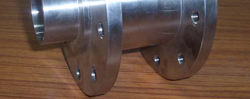
214 Figure B4: Photograph of Tilting pad bearing Figure B5: Photograph of Nozzle_Diffuser Figure B6: Photograph of Bearing housing

215 Figure B7: Photograph of Cold end housing Figure B8: Photograph of Coolant jacket Figure B9: Photograph of Heat exchanger

216 Figure B10: Photograph of all parts of Turboexpander