Periodic Orbits and Transport: Some Interesting Dynamics in the Three-Body Problem

Transcription

1 Periodic Orbits and Transport: Some Interesting Dynamics in the Three-Body Problem Shane Ross Martin Lo (JPL), Wang Sang Koon and Jerrold Marsden (Caltech) CDS 280, January 8, shane/ Control and Dynamical Systems

2 2 Outline Important dynamical objects: Equilibria, periodic orbits, stable and unstable manifolds, bottlenecks Context: Three-body problem (Hamiltonian) Equilibria: Collinear libration points have saddle center structure Periodic orbits: Stable and unstable invariant manifolds divide energy surface, channeling flow in phase space Classification: Interesting orbits can be classified and constructed using Poincaré sections and symbolic dynamics Theorem: Near home/heteroclinic orbits, horseshoe -like dynamics exists Application: Actual space missions

3 Simple Pendulum Connecting Orbits Equations of a simple pendulum are θ + sin θ =0. Write as a system in the plane; dθ dt = v dv dt = sin θ Solutions are trajectories in the plane. The resulting phase portrait shows some important basic features: 5

4 upright pendulum (unstable point) θ = v downward pendulum (stable point) connecting (homoclinic) orbit saddle point θ

5 7 Higher Dimensional Versions are Invariant Manifolds Stable Manifold Unstable Manifold

6 Periodic Orbits Can replace fixed points by periodic orbits and do similar things. For example, stability means nearby orbits stay nearby. 8 x 0 periodic orbit nearby trajectory winding towards the periodic orbit

7 9 Invariant Manifolds for Periodic Orbits Periodic orbits have stable and unstable manifolds. Stable Manifold (orbits move toward the periodic orbit) Unstable Manifold (orbits move away from the periodic orbit)

8 Chaotic Motion and Intermittency 3

9

10 4 Motivation: Comet Transitions Jupiter Comets such as Oterma Comets moving in the vicinity of Jupiter do so mainly under the influence of Jupiter and the Sun i.e., in a three body problem. These comets sometimes make a rapid transition from outside to inside Jupiter s orbit. Captured temporarily by Jupiter during transition. Exterior (2:3 resonance) Interior (3:2 resonance). The next figure shows the orbit of Oterma (AD ) in an inertial frame

11 5 Oterma s orbit 2:3 resonance Second encounter Jupiter y (inertial frame) START Sun 3:2 resonance END First encounter Jupiter s orbit x (inertial frame)

12 Next figure shows Oterma s orbit in a rotating frame (so Jupiter looks like it is standing still) and with some invariant manifolds in the three body problem superimposed. 6

13 7 Homoclinic Orbits Oterma's Trajectory Oterma y (rotating) 1980 Sun L 1 Jupiter L 2 y (rotating) 1910 Jupiter Heteroclinic Connection x (rotating) Boundary of Energy Surface x (rotating)

14 8 Movie: Oterma in a rotating frame

15 Planar Circular Restricted 3-Body Problem PCR3BP General Comments The two main bodies could be the Sun and Jupiter, orthe Sun and Earth, etc. The total mass is normalized to 1; they are denoted m S =1 µand m J = µ, so0<µ 1 2. The two main bodies rotate in the plane in circles counterclockwise about their common center of mass and with angular velocity normalized to 1. The third body, the comet or the spacecraft, has mass zero and is free to move in the plane. The planar restricted three-body problem is used for simplicity. Generalization to the three-dimensional problem is of course important, but many of the effects can be described well with the planar model. 9

16 Equations of Motion Notation: Choose a rotating coordinate system so that the origin is at the center of mass the Sun and Jupiter are on the x-axis at the points ( µ, 0) and (1 µ, 0) respectively i.e., the distance from the Sun to Jupiter is normalized to be 1. Let (x, y) be the position of the comet in the plane relative to the positions of the Sun and Jupiter. distances to the Sun and Jupiter: r 1 = (x + µ) 2 + y 2 and r 2 = (x 1+µ) 2 +y 2. 10

17 11 Y y Comet x Jupiter t Sun X

18 12 y comet y (nondimensional units, rotating frame) x = µ m S = 1 µ Sun r 1 r 2 x = 1 µ m J = µ Jupiter Jupiter's orbit x x (nondimensional units, rotating frame)

19 Lagrangian approach rotating frame: In the rotating frame, the Lagrangian L is given by L(x, y, ẋ, ẏ) = 1 2 ((ẋ y)2 +(x+ẏ) 2 ) U(x, y) where the gravitational potential in rotating coordinates is U = 1 µ r 1 µ r 2. Reason: Ẋ =(ẋ y)cost (x+ẏ)sint, Ẏ =(x+ẏ)cost (ẋ y)sint which yields kinetic energy (wrt inertial frame) Ẋ 2 + Ẏ 2 =(ẋ y) 2 +(x+ẏ) 2. 13

20 Also, since both the distances r 1 and r 2 are invariant under rotation, we have r 2 1 =(x+µ)2 +y 2, r 2 2 =(x (1 µ))2 + y 2. The theory of moving systems says that one can simply write down the Euler-Lagrange equations in the rotating frame and one will get the correct equations. It is a very efficient general method for computing equations for either moving systems or for systems seen from rotating frames (see Marsden & Ratiu, 1999). In the present case, the Euler-Lagrange equations are given by d dt (ẋ y)=x+ẏ U x, d dt (x +ẏ)= ẋ+y U y. 14

21 After simplification, we have the equations of motion: where ẍ 2ẏ= U eff x, U eff = (x2 + y 2 ) 2 ÿ +2ẋ= U eff y 1 µ r 1 µ r 2. They have a first integral, the Hamiltonian energy, given by E(x, y, ẋ, ẏ) = 1 2 (ẋ2 +ẏ 2 )+U eff (x, y). Energy manifolds are 3-dimensional surfaces foliating the 4-dimensional phase space. For fixed energy, Poincaré sections are then 2-dimensional, making visualization of intersections between sets in the phase space particularly simple. 15

22 16 Five Equilibrium Points Three collinear (Euler, 1767) on the x-axis L 1,L 2,L 3 Two equilateral points (Lagrange, 1772) L 4,L 5. y (nondimensional units, rotating frame) L 3 S L 1 J m S = 1 - µ m J = µ L 4 L 5 comet L 2 Jupiter's orbit x (nondimensional units, rotating frame)

23 17 The energy E is given by Energy Manifold E(x, y, ẋ, ẏ) = 1 2 (ẋ2 +ẏ 2 )+U eff (x, y) = 1 2 (ẋ2 +ẏ 2 ) 1 2 (x2 +y 2 ) 1 µ r 1 µ r 2. This energy integral will help us determine the region of possible motion, i.e., the region in which the comet can possibly move along and the region which it is forbidden to move. The first step is to look at the surface of the effective potential U eff. Note that the energy manifold is 3-dimensional.

24 U eff 18

25 Near either the Sun or Jupiter, we have a potential well. Far away from the Sun-Jupiter system, the term that corresponds to the centrifugal force dominates, we have another potential well. Moreover, by applying multivariable calculus, one finds that there are 3 saddle points at L 1,L 2,L 3 and 2 maxima at L 4 and L 5. Let E i be the energy at L i, then E 5 = E 4 >E 3 >E 2 >E 1. 19

26 Let M be the energy surface given by setting the energy integral equal to a constant, i.e., M(µ, e) ={(x, y, ẋ, ẏ) E(x, y, ẋ, ẏ) =e} (1) where e is a constant. The projection of this surface onto position space is called a Hill s region M(µ, e) ={(x, y) U eff (x, y) e}. (2) The boundary of M(µ, e) isthezero velocity curve. The comet can move only within this region in the (x, y)-plane. For a given µthere are five basic configurations for the Hill s region, the first four of which are shown in the following figure. 20

27 21 Case 1 : E<E 1 Case 2 : E 1 <E<E S J S J Case 3 : E 2 <E<E 3 Case 4 : E 3 <E<E 4 =E S J 0 S J

28 [Conley] Orbits with energy just above that of L 2 can be transit orbits, passing through the neck region between the exterior region (outside Jupiter s orbit) and the temporary capture region (bubble surrounding Jupiter). They can also be nontransit orbits or asymptotic orbits. 22 Forbidden Region Exterior Region (X) S L 1 J L 2 L 2 Interior (Sun) Region (S) Jupiter Region (J)

29 23 Flow in the L 1 and L 2 Bottlenecks: Linearization [Moser] All the qualitative results of the linearized equations carry over to the full nonlinear equations. Recall equations of PCR3BP: After linearization, ẋ = v x, ẏ = v y, ẋ = v x, ẏ = v y, v x =2v y U eff x, v y = 2v x U eff y. v x =2v y +ax, v y = 2v x by. Eigenvalues have the form ±λ and ±iν.

30 24 Corresponding eigenvectors are u 1 =(1, σ, λ, λσ), u 2 =(1,σ, λ, λσ), w 1 =(1, iτ, iν, ντ), w 2 =(1,iτ, iν, ντ).

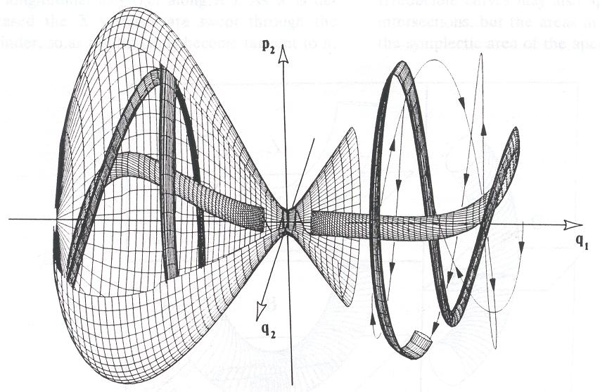
31 After linearization and making the eigenvectors the new coordinate axes, the equations of motion assume the simple form ξ = λξ, η = λη, ζ1 = νζ 2, ζ2 = νζ 1, with energy function E l = ληξ + ν 2 (ζ2 1 + ζ2 2 ). The flow near L 1,L 2 has the form of a saddle center. 25 ξ η ξ=0 ζ 2 =0 η η ξ= c η ξ=+c η+ξ=0 ζ 2 =ρ ζ 2 =0 ζ 2 =ρ

32 For each fixed value of η ξ (vertical lines in figure below), E l = E describes a 2-sphere. The equilibrium region R on the 3D energy manifold is homeomorphic to S 2 I. 26 ξ η ξ=0 ζ 2 =0 η η ξ= c η ξ=+c η+ξ=0 ζ 2 =ρ ζ 2 =0 ζ 2 =ρ

33 27 [McGehee] Can visualize 4typesof orbits in R S 2 I. Black circle is the unstable periodic Lyapunov orbit. 4 cylinders of asymptotic orbits form pieces of stable and unstable manifolds. They intersect the bounding spheres at asymptotic circles, separating spherical polar caps, which contain transit orbits, from spherical equatorial zones, which contain nontransit orbits. Transit Orbits Asymptotic Orbits ω Spherical Cap of Transit Orbits Asymptotic Circle Nontransit Orbits l Spherical Zone of Nontransit Orbits Lyapunov Orbit Cross-section of Equilibrium Region Equilibrium Region

34 Roughly speaking, for fixed energy, the equilibrium region has thedynamicsofasaddle harmonic oscillator. 28 Asymptotic Orbits Transit Orbits ω Spherical Cap of Transit Orbits Asymptotic Circle Nontransit Orbits l Spherical Zone of Nontransit Orbits Lyapunov Orbit Cross-section of Equilibrium Region Equilibrium Region

35 4 cylinders of asymptotic orbits: stable and unstable manifolds. Stable Manifold (orbits move toward the periodic orbit) 29 Unstable Manifold (orbits move away from the periodic orbit)

36 30 Invariant Manifold Tubes Partition the Energy Surface Stable and unstable manifold tubes act as separatrices for the flow in the equilibrium region. Those inside the tubes are transit orbits. Those outside the tubes are nontransit orbits. e.g., transit from outside Jupiter s orbit to Jupiter capture region possible only through L 2 periodic orbit stable tube. Forbidden Region Stable Manifold Jupiter Unstable Manifold Sun L 2 y (rotating frame) Stable Manifold Forbidden Region x (rotating frame) L 2 Periodic Orbit Unstable Manifold

37 Stable and unstable manifold tubes control the transport of material to and from the capture region. 31 Forbidden Region Stable Manifold Jupiter Unstable Manifold Sun L 2 y (rotating frame) Stable Manifold Forbidden Region x (rotating frame) L 2 Periodic Orbit Unstable Manifold

38 32 Tubes of transit orbits contain ballistic capture orbits. Jupiter Comet Begins Inside Tube Sun L 2 y (rotating frame) Ends in Ballistic Capture Passes through L 2 Equilibrium Region x (rotating frame)

39 Invariant manifold tubes are global objects extend far beyond vicinity of libration points. 33 Capture Orbit Tube of Transit Orbits y (rotating frame) Forbidden Region Sun L 2 orbit Jupiter x (rotating frame)

40 Transport between all three regions (interior, Jupiter, exterior) is controlled by the intersection of stable and unstable manifold tubes. 34 X U 3 U 4 U 1 S U 3 J L 1 L 2 J U 2 U 2

41 In particular, rapid transport between outside and inside of Jupiter s orbit is possible. Rapid Transition 35 Exterior Region Forbidden Region Sun Interior Region Jupiter Stable L 1 Manifold Manifold Unstable L 2 Jupiter Region

42 This can be seen by recalling the bounding spheres for the equilibrium regions. We will look at the images and pre-images of the spherical caps of transit orbits on a suitable Poincaré section. The images and pre-images of the spherical caps form the tubes that partition the energy surface. 36 Poincare Section U 3 (x = 1 µ, y > 0 ) d 1,2 + d 2,1 J Stable Manifold Unstable Manifold Right bounding sphere n 1,2 of L 1 equilibrium region (R 1 ) Jupiter region (J ) Left bounding sphere n 2,1 of L 2 equilibrium region (R 2 )

43 For instance, on a Poincaré section between L 1 and L 2, We look at the image of the cap on the left bounding sphere of the L 2 equilibrium region R 2 containing orbits leaving R 2. We also look at the pre-image of the cap on the right bounding sphere of R 1 containing orbits entering R 1. 37

44 The Poincaré cut of the unstable manifold of the L 2 periodic orbit forms the boundary of the image of the cap containing transit orbits leaving R 2. All of these orbits came from the exterior region and are now in the Jupiter region, so we label this region (X; J). Etc. 38 Poincare Section U 3 (x = 1 µ, y > 0 ) d 1,2 + d 2,1 J Stable Manifold Unstable Manifold Right bounding sphere n 1,2 of L 1 equilibrium region (R 1 ) Jupiter region (J ) Left bounding sphere n 2,1 of L 2 equilibrium region (R 2 )

45 Pre-Image of Spherical Cap d 1,2 + (;J,S) y (X;J) Image of Spherical Cap d 2, y Poincare Section U 3 (x = 1 µ, y > 0 ) d 1,2 + d 2,1 J Stable Manifold Unstable Manifold Right bounding sphere n 1,2 of L 1 equilibrium region (R 1 ) Jupiter region (J ) Left bounding sphere n 2,1 of L 2 equilibrium region (R 2 )

46 The dynamics of the invariant manifold tubes naturally suggest the itinerary representation. 40 y (rotating frame) Forbidden Region Forbidden Region Poincare section J L 1 L Stable Unstable 2 Manifold Manifold y (;J,S) Stable Manifold Cut (X;J) Unstable Manifold Cut y (;J,S) (X;J) Intersection Region J = (X;J,S) Stable Manifold Cut Unstable Manifold Cut x (rotating frame) y y

47 Integrating an initial condition in the intersection region would give us an orbit with the desired itinerary (X, J, S). Rapid Transition 41 Exterior Region Forbidden Region Sun Interior Region Jupiter Stable L 1 Manifold Manifold Unstable L 2 Jupiter Region

48 Global Orbit Structure: Overview Found heteroclinic connection between pair of periodic orbits. Find a large class of orbits near this (homo/heteroclinic) chain. Comet can follow these channels in rapid transition. y (AU, Sun-Jupiter rotating frame) Homoclinic Orbit Sun Homoclinic Orbit L1 L 2 Sun Jupiter L 1 L 2 Heteroclinic Connection y (AU, Sun-Jupiter rotating frame) Jupiter s Orbit x (AU, Sun-Jupiter rotating frame) x (AU, Sun-Jupiter rotating frame) -0.8

49 Global Orbit Structure: Energy Manifold Schematic view of energy manifold. y (AU, Sun-Jupiter rotating frame) Homoclinic Orbit Sun Homoclinic Orbit L1 L 2 Sun Jupiter L 1 L 2 Heteroclinic Connection y (AU, Sun-Jupiter rotating frame) Jupiter s Orbit x (AU, Sun-Jupiter rotating frame) x (AU, Sun-Jupiter rotating frame) -0.8 n 1,1 n 1,2 U 3 x = 1 µ n 2,1 n 2,2 a 1,1 a 1,2 + A 2 ' B 2 ' a 2,1 a 2,2 + G 2 ' H 2 ' U 1 y = 0 A 1 B 1 A 1 ' B 1 ' C 1 D 1 + a 1,1 a 1,2 E 1 F 1 G 1 H 1 p 1,2 A 2 B 2 G 1 ' H 1 ' C 2 D 2 + a 2,1 a 2,2 E 2 F 2 G 2 H 2 p 2,2 U 4 y = 0 p 1,1 U 2 x = 1 µ p 2,1 interior region (S ) L 1 equilibrium region (R 1 ) Jupiter region (J ) L 2 equilibrium region (R 2 ) exterior region (X )

50 Global Orbit Structure: Poincaré Map Reducing study of global orbit structure to study of discrete map. n 1,1 n 1,2 U 3 x = 1 µ n 2,1 n 2,2 a 1,1 a 1,2 + A 2 ' B 2 ' a 2,1 a 2,2 + G 2 ' H 2 ' U 1 y = 0 A 1 B 1 A 1 ' B 1 ' C 1 D 1 + a 1,1 a 1,2 E 1 F 1 G 1 H 1 p 1,2 A 2 B 2 G 1 ' H 1 ' C 2 D 2 + a 2,1 a 2,2 E 2 F 2 G 2 H 2 p 2,2 U 4 y = 0 p 1,1 U 2 x = 1 µ p 2,1 interior region (S ) L 1 equilibrium region (R 1 ) Jupiter region (J ) L 2 equilibrium region (R 2 ) exterior region (X ) x = 1 µ U 3 U 1 y = 0 interior region Jupiter region exterior region y = 0 U 4 U 2 D 1 C 1 A 1 ' B 1 ' H 1 ' G 1 ' x = 1 µ C 2 D 2 B 2 ' A 2 ' E 1 F 1 F 2 E 2 G 2 ' H 2 ' U 1 U 2 U 3 U 4

51 Construction of Poincaré Map Construct Poincaré map P (tranversal to the flow) whose domain U consists of 4 squares U i. Squares U 1 and U 4 contained in y =0, each centers around a transversal homoclinic point. Squares U 2 and U 3 contained in x =1 µ, each centers around a transversal heteroclinic point. n 1,1 n 1,2 U 3 x = 1 µ n 2,1 n 2,2 a 1,1 a 1,2 + A 2 ' B 2 ' a 2,1 a 2,2 + G 2 ' H 2 ' U 1 y = 0 A 1 B 1 A 1 ' B 1 ' C 1 D 1 + a 1,1 a 1,2 E 1 F 1 G 1 H 1 p 1,2 A 2 B 2 G 1 ' H 1 ' C 2 D 2 + a 2,1 a 2,2 E 2 F 2 G 2 H 2 p 2,2 U 4 y = 0 p 1,1 U 2 x = 1 µ p 2,1 interior region (S ) L 1 equilibrium region (R 1 ) Jupiter region (J ) L 2 equilibrium region (R 2 ) exterior region (X )

52 Global Orbit Structure near the Chain Consider invariant set Λ of points in U whose images and preimages under all iterations of P remain in U. Λ= n= P n (U). Invariant set Λ contains all recurrent orbits near the chain. It provides insight into the global dynamics around the chain. Chaos theory told us to first consider only the first forward and backward iterations: Λ 1 = P 1 (U) U P 1 (U). U 3 x = 1 µ U 1 y = 0 interior region Jupiter region exterior region y = 0 U 4 U 2 D 1 C 1 A 1 ' B 1 ' H 1 ' G 1 ' x = 1 µ C 2 D 2 B 2 ' A 2 ' E 1 F 1 F 2 E 2 G 2 ' H 2 ' U 1 U 2 U 3 U 4

53 Review of Horseshoe Dynamics: Pendulum

54 Review of Horseshoe Dynamics: Forced Pendulum

55 Review of Horseshoe Dynamics: First Iteration

56 Review of Horseshoe Dynamics: First Iteration

57 Review of Horseshoe Dynamics: Second Iteration

58 Review of Horseshoe Dynamics: Second Iteration...0,0;...1,0;...1,1;...0,1; ;1, ,0;1,1... ;1,1... ;0,1... D ;0,0...

59 Conley-Moser Conditions: Horseshoe-type Map For horseshoe-type map h satisfying Conley-Moser conditions, the invariant set of all iterations, Λ h = n= hn (Q), can be constructed and visualized in a standard way. Strip condition: h maps horizontal strips H 0,H 1 to vertical strips V 0,V 1, (with horizontal boundaries to horizontal boundaries and vertical boundaries to vertical boundaries). Hyperbolicity condition: h has uniform contraction in horizontal direction and expansion in vertical direction....0,0;...1,0;...1,1;...0,1; ;1, ,0;1,1... ;1,1... ;0,1... D ;0,0...

60 Generalized Conley-Moser Conditions Proved P satisfies Generalized Conley-Moser conditions: Strip condition: it maps horizontal strips Hn ij to vertical strips Vn ji. Hyperbolicity condition: it has uniform contraction in horizontal direction and expansion in vertical direction. U 3 E 1 F 1 A 2 ' B 2 ' C 1 E 2 U 1 U 4 D 1 F 2 A 1 ' B 1 ' C 2 G 2 ' H 2 ' D 2 H 1 ' G 1 ' U 2

61 Generalized Conley-Moser Conditions Shown are invariant set Λ 1 under first iteration. Since P satisfies Generalized Conley-Moser Conditions, this process can be repeated ad infinitum. What remains is invariant set of points Λ which are in 1-to-1 corr. with set of bi-infinite sequences (...,u i,m; u j,n,u k,...). U 3 E 1 H n 31 C 1 D 1 A 2 'B 2 ' A 1 ' B 1 ' A 1 'B 1 ' F 1 V m 34 H n 32 V m 32 H 2 C 1 V m 13 H n 11 V m 11 A 2 ' B 2 ' E 2 V m 44 H n 43 V m 42 D 1 H n 12 F 2 H n 44 H 2 C 2 D 2 3;12 Q m;n U 1 C 2 V m 21 H n 23 V m 23 G 2 ' U 4 H 2 ' D 2 H n 24 H 2 H 1 ' U 2 G 1 '

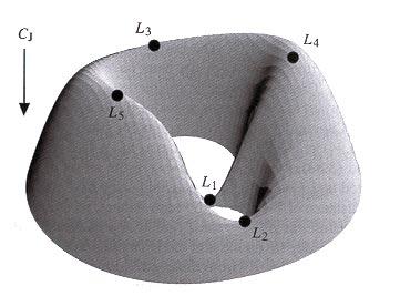
62 Global Orbit Structure: Main Theorem Main Theorem: For any admissible itinerary, e.g., (...,X, 1, J, 0; S, 1, J, 2, X,...), there exists an orbit whose whereabouts matches this itinerary. Can even specify number of revolutions the comet makes around Sun & Jupiter. S L 1 J L 2 X

63 Global Orbit Structure: Dynamical Channels Found a large class of orbits near homo/heteroclinic chain. Comet can follow these channels in rapid transition. y (AU, Sun-Jupiter rotating frame) Homoclinic Orbit Sun Homoclinic Orbit L1 L 2 Sun Jupiter L 1 L 2 Heteroclinic Connection y (AU, Sun-Jupiter rotating frame) Jupiter s Orbit x (AU, Sun-Jupiter rotating frame) x (AU, Sun-Jupiter rotating frame) -0.8

64 42 Lunar Capture: How to get to the Moon Cheaply Using the invariant manifold tubes as the building blocks, we can construct interesting, fuel saving space mission trajectories. For instance, an Earth-to-Moon ballistic capture orbit. Uses Sun s perturbation. Jump from Sun-Earth-S/C system to Earth-Moon-S/C system. Saves about 20% of onboard fuel compared to Apollo-like transfer.

65 43 Maneuver ( V) at Patch Point Earth Targeting Portion Using "Twisting" Lunar Capture Portion Sun y L 2 Moon's Orbit Earth L 2 orbit x

66 Intersection found between Earth-Moon stable manifold and Sun-Earth unstable manifold, which targets trajectory back to Earth. Sun-Earth L 2 Orbit Unstable Manifold Cut Initial Condition Earth Backward Targeting Portion Using "Twisting" 44 y (Sun-Earth rotating frame) Initial Condition Earth-Moon L 2 Orbit Stable Manifold Cut Lunar Capture Portion Sun Moon's Orbit y Earth L 2 L 2 orbit y (Sun-Earth rotating frame) Poincare Section x

67 45 Movie: Shoot the Moon in rotating frame

68 46 Future Research Directions For a single 3-body system: When is 3-body effect more important than 2-body? Find sweet spot within tubes where transport is most efficient/fastest? Consider continuous low-thrust control, optimal control. For coupling multiple 3-body systems: Where to jump from one 3-body system to another? Optimal control: trade off between travel time and fuel. Efficient use of resonances Planetary science/astronomy applications: Statistics: transport rates, capture probabilities, etc. Chemical/atomic physics applications?

69 Final Thought: For a class of Hamiltonian systems which have phase space bottlenecks containing unstable periodic orbits, the unstable and stable manifolds of those periodic orbits partition the part of the energy surface where transport is possible. The manifolds not only provide a picture of the global behavior of the system, but are the starting point for obtaining the statistical properties of the system. 47

70 48 Further Information Koon, W.S., M.W. Lo, J.E. Marsden and S.D. Ross [2000], Heteroclinic connections between periodic orbits and resonance transitions in celestial mechanics, Chaos, vol. 10(2), pp Koon, W.S., M.W. Lo, J.E. Marsden and S.D. Ross [2000], Low energy transfer to the Moon. Jaffé, C., D. Farrelly and T. Uzer [1999], Transition state in atomic physics, Phys. Rev. A, vol. 60(5), pp shane/