CS 188: Artificial Intelligence Learning :

Transcription

1 CS 188: Artificial Intelligence Learning : Instructor: Fabrice Popineau [These slides adapted from Stuart Russell, Dan Klein and Pieter

2 Lectures on learning Learning: a process for improving the performance of an agent through experience Learning I (today): The general idea: generalization from experience Supervised learning: classification and regression Learning II: neural networks and deep learning Learning III: statistical learning and Bayes nets Reinforcement learning II: learning complex V and Q functions

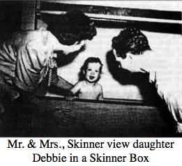
3 Learning: Why? The baby, assailed by eyes, ears, nose, skin, and entrails at once, feels it all as one great blooming, buzzing confusion [William James, 1890] Learning is essential in unknown environments when the agent designer lacks omniscience

4 Learning: Why? Instead of trying to produce a program to simulate the adult mind, why not rather try to produce one which simulates the child's? If this were then subjected to an appropriate course of education one would obtain the adult brain. Presumably the child brain is something like a notebook as one buys it from the stationer's. Rather little mechanism, and lots of blank sheets. [Alan Turing, 1950] Learning is useful as a system construction method, i.e., expose the system to reality rather than trying to write it down

5 Learning: How?

6 Learning: How?

7 Key questions when building a learning agent What is the agent design that will implement the desired performance? Improve the performance of what piece of the agent system and how is that piece represented? What data are available relevant to that piece? (In particular, do we know the right answers?) What knowledge is already available?

8 Examples Agent design Component Representation Feedback Knowledge Alpha-beta search Evaluation function Linear polynomial Win/loss Rules of game; Coefficient signs Logical planning agent Transition model (observable envt) Successor-state axioms Action outcomes Available actions; Argument types Utility-based patient monitor Physiology/senso r model Dynamic Bayesian network Observation sequences Gen physiology; Sensor design Satellite image pixel classifier Classifier (policy) Markov random field Partial labels Coastline; Continuity scales Supervised learning: correct answers for each training instance Reinforcement learning: reward sequence, no correct answers Unsupervised learning: just make sense of the data

9 Supervised learning To learn an unknown target function f Input: a training set of labeled examples (x j,y j ) where y j = f(x j ) E.g., x j is an image, f(x j ) is the label giraffe E.g., x j is a seismic signal, f(x j ) is the label explosion Output: hypothesis h that is close to f, i.e., predicts well on unseen examples ( test set ) Many possible hypothesis families for h Linear models, logistic regression, neural networks, decision trees, examples (nearest-neighbor), grammars, kernelized separators, etc etc Classification = learning f with discrete output value Regression = learning f with real-valued output value

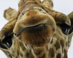
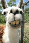
10 Classification example: Object recognition x f(x) giraffe giraffe giraffe llama llama llama X= f(x)=?

11 Regression example: Curve fitting

12 Regression example: Curve fitting

13 Regression example: Curve fitting

14 Regression example: Curve fitting

15 Regression example: Curve fitting

16 Which hypothesis space H to choose? How to measure degree of fit? How to trade off degree of fit vs. complexity? Ockham s razor How do we find a good h? Basic questions How do we know if a good h will predict well?

17 Classification

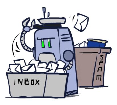
18 Example: Spam Filter Input: an Output: spam/ham Setup: Get a large collection of example s, each labeled spam or ham (by hand) Learn to predict labels of new incoming s Classifiers reject 200 billion spam s per day Features: The attributes used to make the ham / spam decision Words: FREE! Text Patterns: $dd, CAPS Non-text: SenderInContacts, AnchorLinkMismatch Dear Sir. First, I must solicit your confidence in this transaction, this is by virture of its nature as being utterly confidencial and top secret. TO BE REMOVED FROM FUTURE MAILINGS, SIMPLY REPLY TO THIS MESSAGE AND PUT "REMOVE" IN THE SUBJECT. 99 MILLION ADDRESSES FOR ONLY $99 Ok, Iknow this is blatantly OT but I'm beginning to go insane. Had an old Dell Dimension XPS sitting in the corner and decided to put it to use, I know it was working pre being stuck in the corner, but when I plugged it in, hit the power nothing happened.

19 Example: Digit Recognition Input: images / pixel grids Output: a digit 0-9 Setup: MNIST data set of 60K collection hand-labeled imagesnote: someone has to hand label all this data! Want to learn to predict labels of new, future digit images Features: The attributes used to make the digit decision Pixels: (6,8)=ON Shape Patterns: NumComponents, AspectRatio, NumLoops 1??

20 Other Classification Tasks o Classification: given inputs x, predict labels (classes) y o Examples: o Spam detection (input: document, classes: spam / ham) o OCR (input: images, classes: characters) o Medical diagnosis (input: symptoms, classes: diseases) o Automatic essay grading (input: document, classes: grades) o Fraud detection (input: account activity, classes: fraud / no fraud) o Customer service routing o many more o Classification is an important commercial technology!

21 Decision tree models Tree construction Measuring learning performance Decision tree learning

22 Decision trees Popular representation for classifiers Even among humans! I ve just arrived at a restaurant: should I stay (and wait for a table) or go elsewhere?

23 Decision trees It s Friday night and you re hungry You arrive at your favorite cheap but really cool happening burger place It s full up and you have no reservation but there is a bar The host estimates a 45 minute wait There are alternatives nearby but it s raining outside Decision tree partitions the input space, assigns a label to each partition

24 Expressiveness Discrete decision trees can express any function of the input E.g., for Boolean functions, build a path from root to leaf for each row of the truth table: Trivially there is a consistent decision tree that fits any training set exactly (unless true function is nondeterministic) But a tree that simply records the examples is essentially a lookup table To get generalization to new examples, need a compact tree

25 Quiz How many distinct decision trees with n Boolean attributes? = number of distinct Boolean functions with n inputs = number of truth tables with n inputs = number of ways of filling in output column with 2 n entries = 2 2n For n=6 attributes, there are 18,446,744,073,709,551,616 trees

26 Hypothesis spaces in general Increasing the expressiveness of the hypothesis language Increases the chance that the true function can be expressed Increases the number of hypotheses that are consistent with training set => many consistent hypotheses have large test error => may reduce prediction accuracy! With 2 2n hypotheses, all but an exponentially small fraction will require O(2 n ) bits to express in any representation (even brains!) I.e., any given representation can represent only an exponentially small fraction of hypotheses concisely; no universal compression E.g., decision trees are bad at k-out-of-n functions

27 Training data

28 Decision tree learning function Decision-Tree-Learning(examples,attributes,parent_examples) returns a tree if examples is empty then return Plurality-Value(parent_examples) else if all examples have the same classification then return the classification else if attributes is empty then return Plurality-Value(examples) else A argmax a attributes Importance(a, examples) tree a new decision tree with root test A for each value v of A do exs the subset of examples with value v for attribute A subtree Decision-Tree-Learning(exs, attributes A, examples) add a branch to tree with label (A = v k ) and subtree subtree return tree

29 Choosing an attribute: Information gain Idea: measure contribution of attribute to increasing purity of labels in each subset of examples Patrons is a better choice: gives information about classification (i.e., reduces entropy of the distribution of labels)

30 Information answers questions Information The more clueless I am about the answer initially, the more information is contained in the answer Scale: 1 bit = answer to Boolean question with prior 0.5, 0.5 Information in an answer when prior is p 1,,p n is H( p 1,,p n ) = Σ i p i log p i This is the entropy of the prior Convenient notation: B(p) = H( p,1-p )

31 Information gain from splitting on an attribute Suppose we have p positive and n negative examples at the root => B(p/(p+n)) bits needed to classify a new example E.g., for 12 restaurant examples, p = n = 6 so we need 1 bit An attribute splits the examples E into subsets E k, each of which (we hope) needs less information to complete the classification For an example in E k we expect to need B(p k /(p k +n k )) more bits Probability a new example goes into E k is (p k +n k )/(p+n) Expected number of bits needed after split is Σ k (p k +n k )/(p+n) B(p k /(p k +n k )) Information gain = B(p/(p+n)) - Σ k (p k +n k )/(p+n) B(p k /(p k +n k ))

32 Example 1 [(2/12)B(0) + (4/12)B(1) + (6/12)B(2/6)] = bits 1 [(2/12)B(1/2) + (2/12)B(1/2) + = 0 bits (4/12)B(2/6) + (4/12)B(1/2)]

33 Decision tree learned from the 12 examples: Simpler than true tree! Results for restaurant data

34 Training and Testing

35 Basic Concepts Data: labeled instances, e.g. restaurant episodes Training set Validation set Test set Experimentation cycle Generate hypothesis h from training set (Possibly choose best h by trying out on validation set) Finally, compute accuracy of h on test set Very important: never peek at the test set! Evaluation Accuracy: fraction of instances predicted correctly Learning curve: test set accuracy as a function of training set size Training Data Validation Data Test Data

36 Results for restaurant data

37 Linear Regression

38 Linear regression = fitting a straight line/hyperplane 40 h w (x) x Prediction: h w (x) = w 0 + w 1 x Berkeley house prices, 2009

39 Prediction error Error on one instance: y h w (x) Observation y Prediction h w (x) Error or residual x

40 Least squares: Minimizing squared error L2 loss function: sum of squared errors over all examples Loss = Σ j (y j h w (x j )) 2 = Σ j (y j (w 0 + w 1 x j )) 2 We want the weights w* that minimize loss At w* the derivatives of loss w.r.t. each weight are zero: Loss/ w 0 = 2 Σ j (y j (w 0 + w 1 x j )) = 0 Loss/ w 1 = 2 Σ j (y j (w 0 + w 1 x j )) x j = 0 Exact solutions for N examples: w 1 = [NΣ j x j y j (Σ j x j )(Σ j y j )]/[NΣ j x j2 (Σ j x j ) 2 ] and w 0 = 1/N [Σ j y j w 1 Σ j x j ] For the general case where x is an n-dimensional vector X is the data matrix (all the data, one example per row); y is the column of labels w* = (X T X) -1 X T y

41 Summary Learning is essential in unknown environments, useful in many others The nature of the learning process depends on agent design what part of the agent you want to improve what prior knowledge and new experiences are available Supervised learning: learning a function from labeled examples Concise hypotheses generalize better; trade off conciseness and accuracy Classification: discrete-valued function; example: decision trees Regression: real-valued function; example: linear regression Next: neural networks and deep learning

42 CS 188: Artificial Intelligence Naïve Bayes Instructor: Fabrice Popineau [These slides adapted from Stuart Russell, Dan Klein, Pieter Abbeel and Anca

43 Classification

44 Example: Spam Filter o Input: an o Output: spam/ham o Setup: o Get a large collection of example s, each labeled spam or ham o Note: someone has to hand label all this data! o Want to learn to predict labels of new, future s o Features: The attributes used to make the ham / spam decision o Words: FREE! o Text Patterns: $dd, CAPS o Non-text: SenderInContacts o Dear Sir. First, I must solicit your confidence in this transaction, this is by virture of its nature as being utterly confidencial and top secret. TO BE REMOVED FROM FUTURE MAILINGS, SIMPLY REPLY TO THIS MESSAGE AND PUT "REMOVE" IN THE SUBJECT. 99 MILLION ADDRESSES FOR ONLY $99 Ok, Iknow this is blatantly OT but I'm beginning to go insane. Had an old Dell Dimension XPS sitting in the corner and decided to put it to use, I know it was working pre being stuck in the corner, but when I plugged it in, hit the power nothing happened.

45 Example: Digit Recognition o Input: images / pixel grids o Output: a digit 0-9 o Setup: o Get a large collection of example images, each labeled with a digit o Note: someone has to hand label all this data! o Want to learn to predict labels of new, future digit images o Features: The attributes used to make the digit decision o Pixels: (6,8)=ON o Shape Patterns: NumComponents, AspectRatio, NumLoops o 1??

46 Model-Based Classification

47 Model-Based Classification o Model-based approach o Build a model (e.g. Bayes net) where both the label and features are random variables o Instantiate any observed features o Query for the distribution of the label conditioned on the features o Challenges o What structure should the BN have? o How should we learn its parameters?

48 Naïve Bayes for Digits o Naïve Bayes: Assume all features are independent effects of the label o Simple digit recognition version: o One feature (variable) F ij for each grid position <i,j> o Feature values are on / off, based on whether intensity is more or less than 0.5 in underlying image o Each input maps to a feature vector, e.g. F 1 F 2 Y F n o Here: lots of features, each is binary valued o Naïve Bayes model: o What do we need to learn?

49 General Naïve Bayes o A general Naive Bayes model: Y Y parameters F 1 F 2 F n Y x F n values n x F x Y parameters o For each feature we only have to specify how it depends on the class o Total number of parameters is linear in n o Model is very simplistic, but often works anyway

50 Inference for Naïve Bayes o Goal: compute posterior distribution over label variable Y o Step 1: get joint probability of label and evidence for each label + o Step 2: sum to get probability of evidence o Step 3: normalize by dividing Step 1 by Step 2

51 Example: Conditional Probabilities

52 Naïve Bayes for Text o Bag-of-words Naïve Bayes: o Features: W i is the word at positon i o As before: predict label conditioned on feature variables (spam vs. ham) o As before: assume features are conditionally independent given label o New: each W i is identically distributed o Generative model: Word at position i, not i th word in the dictionary! o Tied distributions and bag-of-words o Usually, each variable gets its own conditional probability distribution P(F Y) o In a bag-of-words model o Each position is identically distributed o All positions share the same conditional probs P(W Y) o Why make this assumption? o Called bag-of-words because model is insensitive to word order or reordering

53 Example: Spam Filtering o Model: For numerical stability, work with log instead of actual probability! o What are the parameters? ham : 0.66 spam: 0.33 the : to : and : of : you : a : with: from: the : to : of : : with: from: and : a :

54 Spam Example Word P(w spam) P(w ham) Tot Spam Tot Ham (prior) Gary would you like to lose weight while you sleep P(spam w) = 98.9

55 Example: Spam Filtering o Model: o What are the parameters? ham : 0.66 spam: 0.33 the : to : and : of : you : a : with: from: the : to : of : : with: from: and : a : o Where do these tables come from?

56 General Naïve Bayes o What do we need in order to use Naïve Bayes? o Inference method (we just saw this part) o Start with a bunch of probabilities: P(Y) and the P(F i Y) tables o Use standard inference to compute P(Y F 1 F n ) o Nothing new here o Estimates of local conditional probability tables o P(Y), the prior over labels o P(F i Y) for each feature (evidence variable) o These probabilities are collectively called the parameters of the model and denoted by θ o Up until now, we assumed these appeared by magic, but o they typically come from training data counts

57 Parameter Estimation

58 Parameter Estimation o Estimating the distribution of a random variable o Elicitation: ask a human (why is this hard?) r b b r b b r b b r r b b b b o Empirically: use training data (learning!) o E.g.: for each outcome x, look at the empirical rate of that value: r r b o This is the estimate that maximizes the likelihood of the data

59 Smoothing

60 Maximum Likelihood? o Relative frequencies are the maximum likelihood estimates o Another option is to consider the most likely parameter value given the data????

61 Unseen Events

62 Generalization and Overfitting

63 Overfitting Degree 15 polynomial

64 Example: Overfitting 2 wins!!

65 Example: Overfitting o Posteriors determined by relative probabilities (odds ratios): south-west : inf nation : inf morally : inf nicely : inf extent : inf seriously : inf... screens : inf minute : inf guaranteed : inf $ : inf delivery : inf signature : inf... What went wrong here?

66 Generalization and Overfitting o Relative frequency parameters will overfit the training data! o Just because we never saw a 3 with pixel (15,15) on during training doesn t mean we won t see it at test time o Unlikely that every occurrence of minute is 100% spam o Unlikely that every occurrence of seriously is 100% ham o What about all the words that don t occur in the training set at all? o In general, we can t go around giving unseen events zero probability o As an extreme case, imagine using the entire as the only feature o Would get the training data perfect (if deterministic labeling) o Wouldn t generalize at all o Just making the bag-of-words assumption gives us some generalization, but isn t enough o To generalize better: we need to smooth or regularize the estimates

67 Laplace Smoothing o Laplace s estimate: o Pretend you saw every outcome once more than you actually did r r b o Can derive this estimate with Dirichlet priors (see cs281a)

68 Laplace Smoothing o Laplace s estimate (extended): o Pretend you saw every outcome k extra times r r b o What s Laplace with k = 0? o k is the strength of the prior o Laplace for conditionals: o Smooth each condition independently:

69 Estimation: Linear Interpolation* o In practice, Laplace often performs poorly for P(X Y): o When X is very large o When Y is very large o Another option: linear interpolation o Also get the empirical P(X) from the data o Make sure the estimate of P(X Y) isn t too different from the empirical P(X) o What if α is 0? 1? o For even better ways to estimate parameters, as well as details of the math, see cs281a, cs288

70 Real NB: Smoothing o For real classification problems, smoothing is critical o New odds ratios: helvetica : 11.4 seems : 10.8 group : 10.2 ago : 8.4 areas : verdana : 28.8 Credit : 28.4 ORDER : 27.2 <FONT> : 26.9 money : Do these make more sense?

71 Training and Testing

72 Important Concepts o o o o o Data: labeled instances, e.g. s marked spam/ham o o o Training set Held out set Test set Features: attribute-value pairs which characterize each x Experimentation cycle o o o o Learn parameters (e.g. model probabilities) on training set Tune hyperparameters on held-out set Compute accuracy of test set Very important: never peek at the test set! Evaluation o Accuracy: fraction of instances predicted correctly Overfitting and generalization o o Want a classifier which does well on test data Overfitting: fitting the training data very closely, but not generalizing well Training Data Held-Out Data Test Data

73 Tuning

74 Tuning on Held-Out Data o Now we ve got two kinds of unknowns o Parameters: the probabilities P(X Y), P(Y) o Hyperparameters: e.g. the amount / type of smoothing to do, k, α o What should we learn where? o Learn parameters from training data o Tune hyperparameters on different data o Why? o For each value of the hyperparameters, train and test on the held-out data o Choose the best value and do a final test on the test data

75 Features

76 Errors, and What to Do o Examples of errors Dear GlobalSCAPE Customer, GlobalSCAPE has partnered with ScanSoft to offer you the latest version of OmniPage Pro, for just $99.99* - the regular list price is $499! The most common question we've received about this offer is - Is this genuine? We would like to assure you that this offer is authorized by ScanSoft, is genuine and valid. You can get the To receive your $30 Amazon.com promotional certificate, click through to and see the prominent link for the $30 offer. All details are there. We hope you enjoyed receiving this message. However, if you'd rather not receive future s announcing new store launches, please click...

77 What to Do About Errors? o Need more features words aren t enough! o Have you ed the sender before? o Have 1K other people just gotten the same ? o Is the sending information consistent? o Is the in ALL CAPS? o Do inline URLs point where they say they point? o Does the address you by (your) name? o Can add these information sources as new variables in the NB model o Next class we ll talk about classifiers which let you easily add arbitrary features more easily

78 Baselines o First step: get a baseline o Baselines are very simple straw man procedures o Help determine how hard the task is o Help know what a good accuracy is o Weak baseline: most frequent label classifier o Gives all test instances whatever label was most common in the training set o E.g. for spam filtering, might label everything as ham o Accuracy might be very high if the problem is skewed o E.g. if calling everything ham gets 66%, then a classifier that gets 70% isn t very good o For real research, usually use previous work as a (strong) baseline

79 Confidences from a Classifier o The confidence of a probabilistic classifier: o Posterior over the top label o Represents how sure the classifier is of the classification o Any probabilistic model will have confidences o No guarantee confidence is correct o Calibration o Weak calibration: higher confidences mean higher accuracy o Strong calibration: confidence predicts accuracy rate o What s the value of calibration?

80 Summary o Bayes rule lets us do diagnostic queries with causal probabilities o The naïve Bayes assumption takes all features to be independent given the class label o We can build classifiers out of a naïve Bayes model using training data o Smoothing estimates is important in real systems o Classifier confidences are useful, when you can get them

81 CS 188: Artificial Intelligence Perceptrons Instructor: Fabrice Popineau [These slides adapted from Stuart Russell, Dan Klein, Pieter Abbeel and Anca

82 Regression vs Classification Linear regression when output is binary, yy 0, 1 h ww xx = ww 0 + ww 1 xx y ww 0 + ww 1 xx 1 Linear classification Used with discrete output values Threshold a linear function h ww xx = 1, if ww 0 + ww 1 xx 0 h ww xx = 0, if ww 0 + ww 1 xx < 0 Activation function g 1 y x gg ww 0 + ww 1 xx x

83 Linear Classifiers

84 Feature Vectors Hello, Do you want free printr cartriges? Why pay more when you can get them ABSOLUTELY FREE! Just # free : 2 YOUR_NAME : 0 MISSPELLED : 2 FROM_FRIEND : 0... SPAM or + PIXEL-7,12 : 1 PIXEL-7,13 : 0... NUM_LOOPS :

85 Linear Classifiers o Inputs are feature values o Each feature has a weight o Sum is the activation o If the activation is: o Positive, output +1 o Negative, output 0 f 1 f 2 w 1 w 2 Σ >0? w 3 We can add bias ww 0 f 3

86 Geometric Explanation # free : 4 YOUR_NAME :-1 MISSPELLED : 1 FROM_FRIEND :-3... # free : 2 YOUR_NAME : 0 MISSPELLED : 2 FROM_FRIEND : 0... Dot product positive means the positive class # free : 0 YOUR_NAME : 1 MISSPELLED : 1 FROM_FRIEND : 1...

87 Geometric Explanation o In the space of feature vectors o Examples are points o Any weight vector is a hyperplane o One side corresponds to Y=+1 o Other corresponds to Y=0 money 2 +1 = SPAM BIAS : -3 free : 4 money : = HAM free

88 Weight Updates

89 Perceptron learning rule If true y h w (x) (an error), adjust the weights If w.x < 0 but the output should be y=1 This is called a false negative Should increase weights on positive inputs Should decrease weights on negative inputs If w.x > 0 but the output should be y=0 This is called a false positive Should decrease weights on positive inputs Should increase weights on negative inputs The perceptron learning rule does this: w w + α (y h w (x)) x The perceptron has a default learning rate α=1 Learning rate smaller than 1 is useful in the general case for convergence. See convergence theorem later. learning rate αα ]0, 1] +1, -1, or 0 (no error)

90 Learning: Binary Perceptron o Start with weights = 0 o For each training instance: o Classify with current weights o If correct (i.e., y=y*), no change! o If wrong: adjust the weight vector

91 Learning: Binary Perceptron o Start with weights = 0 o Assume α=1 o For each training instance: o Classify with current weights +1 if ww ff xx 0 yy = 0 if ww ff xx < 0 o If correct (i.e., y=y*), no change! o If wrong: adjust the weight vector by adding or subtracting the feature vector. Subtract if y* is 0.

92 Example y=0 (HAM) money y=1 (SPAM) Bias! free w 0 : -3 w free : 4 w money : 2 x 0 : 1 x free : 1 x money : 1 w.x = -3x1 + 4x1 + 2x1 = 3 Dear Stuart, I wanted to let you know that I have decided to leave Macrosoft and return to academia. The money is is great here but I prefer to be free to pursue more interesting research and I really love teaching undergraduates! Do I need to finish my BA first before applying? Best wishes Bill w w + α (y h w (x)) x α = 0.5 (learning rate) w (-3,4,2) (0 1) (1,1,1) = (-3.5,3.5,1.5)

93 Multiclass Decision Rule o If we have multiple classes: o A weight vector for each class: o Score (activation) of a class y: o Prediction highest score wins Binary = multiclass where the negative class has weight zero

94 Learning: Multiclass Perceptron o Start with all weights = 0 o Assume α=1 o Pick up training examples one by one o Predict with current weights o If correct, no change! o If wrong: lower score of wrong answer, raise score of right answer

95 Example: Multiclass Perceptron win the vote win the election win the game BIAS : 1 win : 0 game : 0 vote : 0 the : 0... BIAS : 0 win : 0 game : 0 vote : 0 the : 0... BIAS : 0 win : 0 game : 0 vote : 0 the : 0...

96 o Separable Case Examples: Perceptron

97 o Non-Separable Case Examples: Perceptron

98 Properties of Perceptrons o Separability: true if some parameters get the training set perfectly correct Separable o Convergence: if the training is separable, perceptron will eventually converge (binary case) o Mistake Bound: the maximum number of mistakes (binary case) related to the margin or degree of separability Non-Separable o kk is the number of features and δδ 2 is the margin (Novikoff, 1962)

99 Perceptron convergence theorem A learning problem is linearly separable iff there is some hyperplane exactly separating +ve from ve examples Separable Convergence: if the training data are separable, perceptron learning applied repeatedly to the training set will eventually converge to a perfect separator Non-Separable This is true with α=1

100 Example: Earthquakes vs nuclear explosions 63 examples, 657 updates required

101 Perceptron convergence theorem A learning problem is linearly separable iff there is some hyperplane exactly separating +ve from ve examples Separable Convergence: if the training data are separable, perceptron learning applied repeatedly to the training set will eventually converge to a perfect separator Convergence: if the training data are non-separable, perceptron learning will converge to a minimum-error solution provided the learning rate α is decayed appropriately (e.g., α=1/t) Non-Separable

102 Perceptron learning with fixed α 71 examples, 100,000 updates fixed αα = 0.2, no convergence

103 Perceptron learning with decaying α 71 examples, 100,000 updates decaying αα = 1000/( tt), near-convergence

104 Improving the Perceptron

105 Problems with the Perceptron o Noise: if the data isn t separable, weights might thrash o Averaging weight vectors over time can help (averaged perceptron) o Mediocre generalization: finds a barely separating solution o Overtraining: test / held-out accuracy usually rises, then falls o Overtraining is a kind of overfitting

106 Fixing the Perceptron o Idea: adjust the weight update to mitigate these effects o MIRA*: choose an update size that fixes the current mistake o but, minimizes the change to w o The +1 helps to generalize * Margin Infused Relaxed Algorithm

107 Minimum Correcting Update min not τ=0, or would not have made an error, so min will be where equality holds

108 Maximum Step Size o In practice, it s also bad to make updates that are too large o Example may be labeled incorrectly o You may not have enough features o Solution: cap the maximum possible value of τ with some constant C o Corresponds to an optimization that assumes non-separable data o Usually converges faster than perceptron o Usually better, especially on noisy data

109 Linear Separators o Which of these linear separators is optimal?

110 Support Vector Machines o Maximizing the margin: good according to intuition, theory, practice o Only support vectors matter; other training examples are ignorable o Support vector machines (SVMs) find the separator with max margin o Basically, SVMs are MIRA where you optimize over all examples at once MIRA SVM

111 Classification: Comparison o Naïve Bayes o Builds a model training data o Gives prediction probabilities o Strong assumptions about feature independence o One pass through data (counting) o Perceptrons / MIRA: o Makes less assumptions about data o Mistake-driven learning o Multiple passes through data (prediction) o Often more accurate

112 Non-Linearity

113 Non-Linear Separators o Data that is linearly separable works out great for linear decision rules: 0 x o But what are we going to do if the dataset is just too hard? 0 x o How about mapping data to a higher-dimensional space: x 2 0 x This and next slide adapted from Ray Mooney, UT

114 Non-Linear Separators General idea: the original feature space can always be mapped to some higherdimensional feature space where the training set is separable: Φ: x φ(x)

115 Neural Networks

116 Very Loose Inspiration: Human Neurons

117 Simple Model of a Neuron (McCulloch & Pitts, 1943) Inputs a i come from the output of node i to this node j (or from outside ) Each input link has a weight w i,j There is an additional fixed input a 0 with bias weight w 0,j The total input is in j = Σ i w i,j a i The output is a j = g(in j ) = g(σ i w i,j a i ) = g(w.a)

118 Single Neuron Single neuron system Perception (if gg is threshold) Logistic regression (if gg is sigmoid) xx 1 ww 1 gg Computed Value aa 1 True Label yy xx 2 ww 2 h ww xx = aa 1 h ww xx = gg ww ii xx ii ii

119 Minimize Single Neuron Loss Data point (xx 1, xx 2 ), label yy Define loss (e.g. quadratic loss) LLLLLLLL ww = (yy h ww (xx)) 2 = (yy gg(dddddd(ww, xx)) 2, gg xx = 1 1+ee xx, dddddd xx, ww = ii ww ii xx ii Compute partial derivative LLLLLLLL ww = ww ii gg dddddd dddddd ww ii Step each weight along (negative) derivative of loss function Gradient descent w i = w ii αα ww ii LLLLLLLL ww LLLLLLss qqqqqqqqqqqqqqqqqq xx, yy = yy xx 2

120 Choice of Activation Function It would be really helpful to have a g(z) that was nicely differentiable Hard threshold: gg zz = 1 zz 0 0 zz < 0 dddd dddd = 0 zz 0 0 zz < 0 Sigmoid: gg zz gg zz = 1 1+ee zz dddd dddd = gg xx 1 gg zz ReLU: gg zz = mmmmmm(0, zz) dddd dddd = 1 zz 0 0 zz < 0

121 Multiclass Classification How do we handle labels that have more than two values? For example, classifying handwritten digits 0-9 One vs. Rest: Train NN binary classifiers For each class ii, Train a binary classifier where the new labels are 1 if label = ii, and 0 otherwise If the classfication score from binary classifier ii is higher than the other NN 1 classifiers, then label the point as label ii.

122 Multiclass Classification How do we handle labels that have more than two values? For example, classifying handwritten digits 0-9 Softmax Generalization of the sigmoid function to multiple classes NN inputs and NN outputs Give a probability that the input data produced each class The NN softmax outputs sum to 1 gg ssssssssssssss xx, ii = eexx ii jj ee xx jj xx 1 aa 11 ww 113 ww 111 ww 112 softmax function aa21 ww 121 xx 2 aa 12 gg aa 22 ww 123 aa 22 ww 131 xx 3 aa 13 ww 133

123 Multilayer Perceptrons A multilayer perceptron is a feedforward neural network with at least one hidden layer (nodes that are neither inputs nor outputs) MLPs with enough hidden nodes can represent any function

124 Neural Network Equations xx 1 aa 11 ww 111 gg aa 21 ww 211 aa 31 ww 112 ww 113 ww 212 gg ww 311 xx 2 aa 12 ww 121 gg aa 22 ww 221 gg aa 41 ww 123 ww 131 ww 221 gg aa 32 ww 321 xx 3 aa 13 w 133 gg aa 23 ww 232 h ww xx = aa 4,1 aa 1,1 = xx 1 aa 4,1 = gg ii ww 3,ii,1 aa 3,ii aa 3,1 = gg ii ww 2,ii,1 aa 2,ii h ww xx = gg ww 3,kk,1 gg kk jj ww 2,jj,kk gg ww 1,ii,jj xx ii ii aa l,1 = gg ii ww l 1,ii,1 aa l 1,ii

125 Minimize Neural Network Loss Data point (xx 1, xx 2 ), label yy Define loss (e.g. quadratic loss) LLLLLLLL ww = (yy h ww (xx)) 2 = yy gg ii ww LL,ii,1 aa LL,ii 2 Compute partial derivative LLLLLLLL ww = ww l,mm,nn gg = yy gg ww ii ww LL,ii,1 aa LL,ii l,mm,nn ww l,mm,nn Step each weight along (negative) derivative of loss function Gradient descent w l,mm,nn = w l,mm,nn αα ww l,mm,nn LLLLLLLL ww

126 Error Backpropagation Δ 3 = ggg(iiii 3 ) [ww 3, 5Δ 5 + ww 3, 6Δ 6 ] Δ 5 = ggg(iiii 5 ) (yy 5 aa 5 ) Δ 6 = ggg(iiii 6 ) (yy 6 aa 6 ) a 22 Δ 4 = ggg(iiii 4 ) [ww 4, 5Δ 5 + ww 4, 6Δ 6 ]

127 Represent as Computational Graph x * s (scores) hinge loss + L W R 141

128 e.g. x = -2, y = 5, z =

129 e.g. x = -2, y = 5, z = -4 Want: 143

130 e.g. x = -2, y = 5, z = -4 Want: 144

131 e.g. x = -2, y = 5, z = -4 Want: 145

132 e.g. x = -2, y = 5, z = -4 Want: 146

133 e.g. x = -2, y = 5, z = -4 Want: 147

134 e.g. x = -2, y = 5, z = -4 Want: 148

135 e.g. x = -2, y = 5, z = -4 Want: 149

136 e.g. x = -2, y = 5, z = -4 Want: 150

137 e.g. x = -2, y = 5, z = -4 Chain rule: Want: 151

138 e.g. x = -2, y = 5, z = -4 Want: 152

139 e.g. x = -2, y = 5, z = -4 Chain rule: Want: 153

140 activations f 154

141 activations local gradient f 155

142 activations local gradient f gradients 156

143 activations local gradient f gradients 157

144 activations local gradient f gradients 158

145 activations local gradient f gradients 159

146 Another example: 160

147 Another example: 161

148 Another example: 162

149 Another example: 163

150 Another example: 164

151 Another example: 165

152 Another example: 166

153 Another example: 167

154 Another example: 168

155 Another example: (-1) * (-0.20) =

156 Another example: 170

157 Another example: [local gradient] x [its gradient] [1] x [0.2] = 0.2 [1] x [0.2] = 0.2 (both inputs!) 171

158 Another example: 172

159 Another example: [local gradient] x [its gradient] x0: [2] x [0.2] = 0.4 w0: [-1] x [0.2] =

160 sigmoid function sigmoid gate 174

161 sigmoid function sigmoid gate (0.73) * (1-0.73) =

162 Gradients add at branches + 176

163 Mini-batches and Stochastic Gradient Descent o Typical objective: = average log-likelihood of label given input = estimate based on mini-batch 1 k - Mini-batch gradient descent: compute gradient on mini-batch (+ cycle over mini-batches: 1..k, k+1 2k,... ; make sure to randomize permutation of data!) - Stochastic gradient descent: k = 1

164 CS 188: Artificial Intelligence Deep Learning Instructor: Fabrice Popineau [These slides adapted from Stuart Russell, Dan Klein, Pieter Abbeel and Anca

165 Computer Vision

166 Object Detection

167 Manual Feature Design

168 Features and Generalization [Dalal and Triggs, 2005]

169 Features and Generalization Image HoG

170 Manual Feature Design Deep Learning o Manual feature design requires: o Domain-specific expertise o Domain-specific effort o What if we could learn the features, too? o -> Deep Learning

171 Performance graph credit Matt Zeiler, Clarifai

172 Performance graph credit Matt Zeiler, Clarifai

173 graph credit Matt Zeiler, Clarifai Performance AlexNet

174 graph credit Matt Zeiler, Clarifai Performance AlexNet

175 graph credit Matt Zeiler, Clarifai Performance AlexNet

176 Speech Recognition graph credit Matt Zeiler, Clarifai

177 Speech Synthesis: WaveNet WaveNet (2016) Approach for the Text to Speech problem (TTS). Concatenative TTS: Short recorded speech fragments concatenated. Parametric TTS: High level model based speech generation (from scratch). WaveNet: Dumb neural network based model for generating human speech at the level of individual audio samples. (Note: This is not a classifier! Not a direct application of today s ideas, but instead an example of the generality of deep neural networks)

178 Deep Learning: Convolutional Neural Networks LeNet5 Lecun, et al, 1998 Convnets for digit recognition LeCun, Yann, et al. "Gradient-based learning applied to document recognition." Proceedings of the IEEE (1998):

179 Convolutional Neural Networks Alexnet Alex Krizhevsky, Geoffrey Hinton, et al, 2012 Convnets for image classification More data & more compute power Krizhevsky, Alex, Ilya Sutskever, and Geoffrey E. Hinton. "Imagenet classification with deep convolutional neural networks." Advances in neural information processing systems

180 Deep Learning: GoogLeNet Szegedy, Christian, et al. Going deeper with convolutions." CVPR (2015).

181 Neural Nets Incredible success in the last three years Data (ImageNet) Compute power Optimization Activation functions (ReLU) Regularization Reducing overfitting (dropout) Software packages Caffe (UC Berkeley) Theano (Université de Montréal) Torch (Facebook, Yann Lecun) TensorFlow (Google)

182 Practical Issues