The Spectral Method (MAPH 40260)

Transcription

1 The Spectral Method (MAPH 40260) Part 4: Barotropic Vorticity Equation Peter Lynch School of Mathematical Sciences

2 Outline Background Rossby-Haurwitz Waves Interaction Coefficients Transform Method The ECMWF Model

3 Outline Background Rossby-Haurwitz Waves Interaction Coefficients Transform Method The ECMWF Model

4 The dynamics of non-divergent flow on a rotating sphere are described by the conservation of absolute vorticity.

5 The dynamics of non-divergent flow on a rotating sphere are described by the conservation of absolute vorticity. The analytical study of the nonlinear barotropic vorticity equation is greatly facilitated by the expansion of the solution in spherical harmonics.

6 The dynamics of non-divergent flow on a rotating sphere are described by the conservation of absolute vorticity. The analytical study of the nonlinear barotropic vorticity equation is greatly facilitated by the expansion of the solution in spherical harmonics. The normal modes are the well-known Rossby-Haurwitz (RH) waves which represent the natural oscillations of the system.

7 The dynamics of non-divergent flow on a rotating sphere are described by the conservation of absolute vorticity. The analytical study of the nonlinear barotropic vorticity equation is greatly facilitated by the expansion of the solution in spherical harmonics. The normal modes are the well-known Rossby-Haurwitz (RH) waves which represent the natural oscillations of the system. Triads of RH waves that satisfy conditions for resonance are of critical importance for the distribution of energy in the atmosphere.

8 The dynamical behaviour of planetary waves in the atmosphere is modelled by the barotropic vorticity equation (BVE): d(ζ + f ) = 0. dt

9 The dynamical behaviour of planetary waves in the atmosphere is modelled by the barotropic vorticity equation (BVE): d(ζ + f ) = 0. dt Rossby (1939) used a simplified (linear) form of this equation for his study of atmospheric waves. This was generalized to spherical geometry by Haurwitz (1940). The linear wave solutions are now called Rossby-Haurwitz waves.

10 The dynamical behaviour of planetary waves in the atmosphere is modelled by the barotropic vorticity equation (BVE): d(ζ + f ) = 0. dt Rossby (1939) used a simplified (linear) form of this equation for his study of atmospheric waves. This was generalized to spherical geometry by Haurwitz (1940). The linear wave solutions are now called Rossby-Haurwitz waves. Charney, Fjørtoft & von Neumann (1950) integrated the BVE to produce the earliest numerical weather predictions on the ENIAC. They integrated the equation on a rectangular domain, in planar geometry.

11 Silberman(1954) devised a numerical solution method in which the streamfunction is expanded in spherical surface harmonics. The nonlinear terms introduced interaction coefficients between the components.

12 Silberman(1954) devised a numerical solution method in which the streamfunction is expanded in spherical surface harmonics. The nonlinear terms introduced interaction coefficients between the components. A more efficient spectral technique, the transform method, was later devised by Eliasen, Machenhauer and Rasmussen (1970) and by Orszag (1970).

13 Silberman(1954) devised a numerical solution method in which the streamfunction is expanded in spherical surface harmonics. The nonlinear terms introduced interaction coefficients between the components. A more efficient spectral technique, the transform method, was later devised by Eliasen, Machenhauer and Rasmussen (1970) and by Orszag (1970). Highly truncated versions of the spectral BVE have been analysed to gain understanding of atmospheric phenomena. Edward Lorenz (1960) introduced what he called the maximum simplification of the system, reducing it to three nonlinear ODEs.

14 In a series of papers, George Platzman undertook a systematic study of the truncated spectral vorticity equation (Platzman, 1960, 1962). He showed that a three-component system has periodic solutions: the equations are integrable and the solutions are expressible in terms of Jacobi elliptic functions.

15 In a series of papers, George Platzman undertook a systematic study of the truncated spectral vorticity equation (Platzman, 1960, 1962). He showed that a three-component system has periodic solutions: the equations are integrable and the solutions are expressible in terms of Jacobi elliptic functions. Interactions are particularly effective when the component parameters are related by resonance conditions.

16 The nonlinear interactions between different scales play a critical role in establishing the statistical energy spectrum of the atmosphere.

17 The nonlinear interactions between different scales play a critical role in establishing the statistical energy spectrum of the atmosphere. The phenomenon of vacillation in the stratospheric flow was first examined by Holton & Mass (1976). They found that, for wave forcing beyond a critical amplitude, the response to a steady forcing is not steady, but the mean zonal flow and eddy components oscillate quasi-periodically.

18 The nonlinear interactions between different scales play a critical role in establishing the statistical energy spectrum of the atmosphere. The phenomenon of vacillation in the stratospheric flow was first examined by Holton & Mass (1976). They found that, for wave forcing beyond a critical amplitude, the response to a steady forcing is not steady, but the mean zonal flow and eddy components oscillate quasi-periodically. Such oscillatory response to steady forcing is consistent with forced resonant triads (Lynch, 2009).

19 Outline Background Rossby-Haurwitz Waves Interaction Coefficients Transform Method The ECMWF Model

20

21 In this section, we review the spectral analysis of the BVE, and the normal mode solutions of the equation.

22 In this section, we review the spectral analysis of the BVE, and the normal mode solutions of the equation. We consider a shallow layer of incompressible fluid on a rotating sphere, assuming the horizontal velocity to be non-divergent. The radius of the sphere is a, the rotation rate is Ω and longitude/latitude coordinates (λ, φ) will be used.

23 In this section, we review the spectral analysis of the BVE, and the normal mode solutions of the equation. We consider a shallow layer of incompressible fluid on a rotating sphere, assuming the horizontal velocity to be non-divergent. The radius of the sphere is a, the rotation rate is Ω and longitude/latitude coordinates (λ, φ) will be used. The dynamics of the fluid are governed by conservation of absolute vorticity d dt (ζ + f ) = 0, where f = 2Ω sin φ is the planetary vorticity, and ζ = k V is the vorticity of the flow.

24 The time derivative is dζ = ζ dt t + u ζ a cos φ λ + v ζ a φ. We assume nondivergent flow and introduce a stream-function ψ such that V = k ψ and ζ = 2 ψ.

25 The time derivative is dζ = ζ dt t + u ζ a cos φ λ + v ζ a φ. We assume nondivergent flow and introduce a stream-function ψ such that V = k ψ and ζ = 2 ψ. The advection term now becomes dζ = ζ dt t 1 ψ 1 ζ a φ a cos φ λ + 1 ψ 1 ζ a cos φ λ a φ.

26 The time derivative is dζ = ζ dt t + u ζ a cos φ λ + v ζ a φ. We assume nondivergent flow and introduce a stream-function ψ such that V = k ψ and ζ = 2 ψ. The advection term now becomes dζ = ζ dt t 1 ψ 1 ζ a φ a cos φ λ + 1 ψ 1 ζ a cos φ λ a φ. Defining µ = sin φ, this may be expressed as dζ = ζ dt t + 1 [ ψ ζ a 2 µ λ + ψ ] ζ λ µ = ζ t + 1 (ψ, ζ) a 2 (λ, µ) = ζ t + 1 J(ψ, ζ). a2

27 Since f = 2Ω sin φ, the β-term may be expressed df dt = v f a φ 1 ψ 1 f = a cos φ λ a φ 1 ψ 1 2Ω ψ = 2Ω cos φ = a cos φ λ a a 2 λ

28 Since f = 2Ω sin φ, the β-term may be expressed df dt = v f a φ 1 ψ 1 f = a cos φ λ a φ 1 ψ 1 2Ω ψ = 2Ω cos φ = a cos φ λ a a 2 λ The barotropic vorticity equation may now be written ζ t + 2Ω a 2 ψ λ + 1 a 2 (ψ, ζ) (λ, µ) = 0 This is the (non-divergent) BVE.

29 The non-linear advection is represented by the Jacobian term.

30 The non-linear advection is represented by the Jacobian term. Temporarily omitting this, we see that the BVE has solutions of the form ψ = ψ 0 Y m n (λ, µ) exp( iσt) where ψ 0 is the constant amplitude and the frequency σ is given by the dispersion formula σ = σ m n 2Ωm n(n + 1).

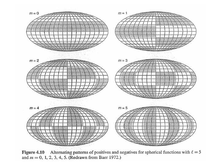
31 The non-linear advection is represented by the Jacobian term. Temporarily omitting this, we see that the BVE has solutions of the form ψ = ψ 0 Y m n (λ, µ) exp( iσt) where ψ 0 is the constant amplitude and the frequency σ is given by the dispersion formula σ = σ m n 2Ωm n(n + 1). Here, m is the zonal wavenumber, n is the total wavenumber (both are integers) and Y m n (λ, µ) are the spherical harmonics, eigenfunctions of 2 : 2 Yn m n(n + 1) = Y m a 2 n.

32 We assume the functions Yn m to be normalized so that 1 (Y m 1 n 4π 1 ) Y m 2 n 2 dλdµ = δ m 1 m 2 δ n 1 n 2. These solutions are called Rossby-Haurwitz waves, or RH waves.

33 We assume the functions Yn m to be normalized so that 1 (Y m 1 n 4π 1 ) Y m 2 n 2 dλdµ = δ m 1 m 2 δ n 1 n 2. These solutions are called Rossby-Haurwitz waves, or RH waves. It is remarkable that, for a single RH wave, the nonlinear Jacobian term vanishes identically, so that such a wave is a solution of the nonlinear BVE.

34 Outline Background Rossby-Haurwitz Waves Interaction Coefficients Transform Method The ECMWF Model

35 The spherical harmonics form an orthonormal basis on the sphere: any sufficiently smooth function may be expressed as a sum of such components.

36 The spherical harmonics form an orthonormal basis on the sphere: any sufficiently smooth function may be expressed as a sum of such components. Thus, the streamfunction has an expansion ψ(λ, µ, t) = n ψn m (t)yn m (λ, µ). n=0 m= n

37 The spherical harmonics form an orthonormal basis on the sphere: any sufficiently smooth function may be expressed as a sum of such components. Thus, the streamfunction has an expansion ψ(λ, µ, t) = n ψn m (t)yn m (λ, µ). n=0 m= n The vorticity has a similar expansion, with coefficients ζn m n(n + 1) = ψ m a 2 n.

38 The spherical harmonics form an orthonormal basis on the sphere: any sufficiently smooth function may be expressed as a sum of such components. Thus, the streamfunction has an expansion ψ(λ, µ, t) = n ψn m (t)yn m (λ, µ). n=0 m= n The vorticity has a similar expansion, with coefficients ζn m n(n + 1) = ψ m a 2 n. The coefficients ψ m n and ζ m n are functions of time.

39 Flows governed by the BVE conserve the total energy and total enstrophy, defined by E = V Vdλ dµ = ψζ dλ dµ 4πa 2 2 4πa 2 2 S = 1 4πa ζ2 dλ dµ = 1 4πa 2 1 ψ ζ dλ dµ 2

40 Flows governed by the BVE conserve the total energy and total enstrophy, defined by E = V Vdλ dµ = ψζ dλ dµ 4πa 2 2 4πa 2 2 S = 1 4πa ζ2 dλ dµ = 1 4πa 2 1 ψ ζ dλ dµ 2 In terms of the spectral coefficients, the constrained quantities may be written E = 1 2 mn 1 n(n + 1) ζm n 2, S = 1 2 ζ mn 2. mn

41 Flows governed by the BVE conserve the total energy and total enstrophy, defined by E = V Vdλ dµ = ψζ dλ dµ 4πa 2 2 4πa 2 2 S = 1 4πa ζ2 dλ dµ = 1 4πa 2 1 ψ ζ dλ dµ 2 In terms of the spectral coefficients, the constrained quantities may be written E = 1 2 mn 1 n(n + 1) ζm n 2, S = 1 2 ζ mn 2. The constancy of energy and enstrophy profoundly influences the energetics of solutions of the BVE. mn

42 For brevity we define a vector wavenumber γ = (m, n) and denote its conjugate by γ = ( m, n).

43 For brevity we define a vector wavenumber γ = (m, n) and denote its conjugate by γ = ( m, n). We can then write the expansions ψ = γ ψ γ (t)y γ (λ, µ) exp( iσ γ t) and ζ = γ ζ γ (t)y γ (λ, µ) exp( iσ γ t) with ψ γ = a 2 κ γ ζ γ, where κ γ = 1 n(n + 1)

44 For brevity we define a vector wavenumber γ = (m, n) and denote its conjugate by γ = ( m, n). We can then write the expansions ψ = γ ψ γ (t)y γ (λ, µ) exp( iσ γ t) and ζ = γ ζ γ (t)y γ (λ, µ) exp( iσ γ t) with ψ γ = a 2 κ γ ζ γ, where κ γ = 1 n(n + 1) For a pure RH wave, or a collection of non-interacting waves, the coefficients ψ γ and ζ γ are constants. Their variation is due to nonlinear interactions between the components.

45 If the expansion ζ = γ ζ γ (t)y γ (λ, µ) exp( iσ γ t) is substituted into the BVE and the orthogonality condition is used, we obtain equations for the evolution of the spectral coefficients in time: dζ γ dt = 1 2 i α,β I γβα ζ β ζ α exp( iσt),

46 If the expansion ζ = γ ζ γ (t)y γ (λ, µ) exp( iσ γ t) is substituted into the BVE and the orthogonality condition is used, we obtain equations for the evolution of the spectral coefficients in time: dζ γ dt = 1 2 i α,β I γβα ζ β ζ α exp( iσt), Here σ = σ α + σ β σ γ and the interaction coefficients are given by I γβα = (κ β κ α )K γβα.

47 The coupling integrals K γβα vanish unless m α + m β = m γ ; this follows from the separability of the spherical harmonics and the orthogonality of the exponential components for different m.

48 The coupling integrals K γβα vanish unless m α + m β = m γ ; this follows from the separability of the spherical harmonics and the orthogonality of the exponential components for different m. In case m α + m β = m γ, they are given by K γβα = ( ) dp α P γ m β P β dµ m dp β αp α dµ. dµ The interaction coefficients vanish in most cases. For non-vanishing interaction, selection rules must be satisfied...

49 Selection Rules m α + m β = m γ m 2 α + m 2 β 0 n γ n β n α 0 n α n β n α + n β + n γ is odd (n β m β ) 2 + (n α m α ) 2 0 n α n β < n γ < n α + n β (m β, n β ) ( m γ, n γ ) and (m α, n α ) ( m γ, n γ )

50 It is obvious that the following symmetries hold: I γαβ = I γβα and K γαβ = K γβα.

51 It is obvious that the following symmetries hold: I γαβ = I γβα and K γαβ = K γβα. The following redundancy rules are easily proved by integration by parts: K α βγ = K γβα and K βγᾱ = K γβα, where ᾱ = ( m, n) when α = (m, n).

52 Outline Background Rossby-Haurwitz Waves Interaction Coefficients Transform Method The ECMWF Model

53 The Transform Method The interaction coefficients grow rapidly in number with increasing truncation. Thus, this method is not normally used to solve the spectral equations.

54 The Transform Method The interaction coefficients grow rapidly in number with increasing truncation. Thus, this method is not normally used to solve the spectral equations. A more efficient spectral technique, the transform method, was devised by Eliasen, Machenhauer and Rasmussen (1970) and, independently, by Orszag (1970).

55 The Transform Method The interaction coefficients grow rapidly in number with increasing truncation. Thus, this method is not normally used to solve the spectral equations. A more efficient spectral technique, the transform method, was devised by Eliasen, Machenhauer and Rasmussen (1970) and, independently, by Orszag (1970). In this approach, the fields are transformed, at each time step, back to the physical domain, the nonlinear terms are calculated, and the result is transformed to spectral space.

56 Pros and Cons of Spectral Method Pros: Spatial derivatives evaluated exactly. Energy and enstrophy exactly conserved. Uniform resolution throughout sphere.

57 Pros and Cons of Spectral Method Pros: Spatial derivatives evaluated exactly. Energy and enstrophy exactly conserved. Uniform resolution throughout sphere. Cons: Less direct than finite difference method. Interaction coefficient method expensive.

58 Pros and Cons of Spectral Method Pros: Spatial derivatives evaluated exactly. Energy and enstrophy exactly conserved. Uniform resolution throughout sphere. Cons: Less direct than finite difference method. Interaction coefficient method expensive. The transform method addresses the last point.

59

60 Derivatives are evaluated exactly in spectral space. The nonlinear terms involve products of derivatives, e.g., u ζ x = 1 ψ ζ a µ x.

61 Derivatives are evaluated exactly in spectral space. The nonlinear terms involve products of derivatives, e.g., u ζ x = 1 ψ ζ a µ x. The essence of the transform method is this: The spatial derivatives are evaluated in spectral space. These are then transformed to gridpoint space. The multiplications etc. are done in gridpoint space. The resulting nonlinear terms are transformed back to spectral space.

62 To make this concrete, consider the term ζ x

63 To make this concrete, consider the term ζ x We have the vorticity in spectral space N +n ζ = Zn m Yn m (λµ) n=0 m= n

64 To make this concrete, consider the term ζ x We have the vorticity in spectral space N +n ζ = Zn m Yn m (λµ) n=0 m= n The x-derivative of this is N ζ x = +n (im)zn m Yn m (λµ) n=0 m= n i.e. the coefficients are (im)z m n.

65 To make this concrete, consider the term ζ x We have the vorticity in spectral space N +n ζ = Zn m Yn m (λµ) n=0 m= n The x-derivative of this is N ζ x = +n (im)zn m Yn m (λµ) n=0 m= n i.e. the coefficients are (im)z m n. This transform gives the values in gridpoint space.

66 To make this concrete, consider the term ζ x We have the vorticity in spectral space N +n ζ = Zn m Yn m (λµ) n=0 m= n The x-derivative of this is N ζ x = +n (im)zn m Yn m (λµ) n=0 m= n i.e. the coefficients are (im)z m n. This transform gives the values in gridpoint space. We do this for all the terms, do the multiplications, and transform back to spectral space.

67 The invention of the transform method revolutionized the use of the spectral method. From being a method primarily of theoretical interest, it became a method of great practical interest.

68 The invention of the transform method revolutionized the use of the spectral method. From being a method primarily of theoretical interest, it became a method of great practical interest. The method is at the heart of most global models of the atmosphere, for example, the ECMWF model known as the IFS code.

69

70

71 Outline Background Rossby-Haurwitz Waves Interaction Coefficients Transform Method The ECMWF Model

72 Perhaps the most important event in European meteorology over the last half-century was the establishment of the European Centre for Medium-Range Weather Forecasts (ECMWF).

73 Perhaps the most important event in European meteorology over the last half-century was the establishment of the European Centre for Medium-Range Weather Forecasts (ECMWF). The mission of the Centre is to deliver weather forecasts of increasingly high quality and scope from a few days to a few seasons ahead.

74 Perhaps the most important event in European meteorology over the last half-century was the establishment of the European Centre for Medium-Range Weather Forecasts (ECMWF). The mission of the Centre is to deliver weather forecasts of increasingly high quality and scope from a few days to a few seasons ahead. The Centre has been spectacularly successful in fulfilling its mission, and continues to develop forecasts and other products of steadily increasing accuracy and value, maintaining its position as a world leader.

75 ECMWF produces a wide range of global atmospheric and marine forecasts and disseminates them on a regular schedule to its Member States.

76 ECMWF produces a wide range of global atmospheric and marine forecasts and disseminates them on a regular schedule to its Member States. Forecasts for the atmosphere out to ten days ahead, based on a T799 (25 km) 91-level (L91) deterministic model are disseminated twice per day. Forecasts from the Ensemble Prediction System (EPS) using a T399 (50 km) L62 version of the model and an ensemble of fifty-one members are computed and disseminated twice per day. Forecasts out to one month ahead, based on ensembles using a resolution of T255 (78 km) and 62 levels are distributed once per week. Seasonal Forecasts out to six months ahead, based on ensembles with a T159 (125 km) L40 model are disseminated once per month.

77 The Integrated Forecast System The basis of the NWP operations at ECMWF is the Integrated Forecast System (IFS).

78 The Integrated Forecast System The basis of the NWP operations at ECMWF is the Integrated Forecast System (IFS). The IFS uses a spectral representation of the meteorological fields. Each field is expanded in series of spherical harmonics; for example, n u(λ, φ, t) = Un m (t)yn m (λ, φ) n=0 m= n where the coefficients U m n (t) depend only on time, and the spherical harmonics Y m n (λ, φ) are as introduced above.

79 The Integrated Forecast System The basis of the NWP operations at ECMWF is the Integrated Forecast System (IFS). The IFS uses a spectral representation of the meteorological fields. Each field is expanded in series of spherical harmonics; for example, n u(λ, φ, t) = Un m (t)yn m (λ, φ) n=0 m= n where the coefficients U m n (t) depend only on time, and the spherical harmonics Y m n (λ, φ) are as introduced above. The coefficients Un m of the harmonics provide an alternative to specifying the field values u(λ, φ) in the spatial domain.

80 It is straightforward to transform back and forth between physical space and spectral space.

81 It is straightforward to transform back and forth between physical space and spectral space. When the model equations are transformed to spectral space, they become a set of equations for the spectral coefficients U m n. These are used to advance the coefficients in time, after which the new physical fields may be computed.

82 Triangular Truncation A continuous field in space requires an infinite series expansion. The series expansion must be truncated at some point.

83 Triangular Truncation A continuous field in space requires an infinite series expansion. The series expansion must be truncated at some point. In the IFS model, the expansion is truncated at a fixed total wavenumber N: u(λ i, φ j, t) = N n Un m (t)yn m (λ i, φ j ) n=0 m= n This is called triangular truncation, and the value of N indicates the resolution of the model. E.g., if N = 512, the resolution is denoted T 512.

84 There is a computational grid, called the Gaussian grid, corresponding to the spectral truncation.

85 There is a computational grid, called the Gaussian grid, corresponding to the spectral truncation. Since truncation at wavenumber N implies a maximum of N wavelengths around the globe, and since at least two points per wavelength are required, the resolution of the equivalent Gaussian grid is given by the circumference of the Earth divided by twice the truncation N, that is, = (2πa)/2N.

86 There is a computational grid, called the Gaussian grid, corresponding to the spectral truncation. Since truncation at wavenumber N implies a maximum of N wavelengths around the globe, and since at least two points per wavelength are required, the resolution of the equivalent Gaussian grid is given by the circumference of the Earth divided by twice the truncation N, that is, = (2πa)/2N. Since 2πa = m, we get the simple rule ( ) 20,000 = km. N

87 Table: Upgrade to the ECMWF Integrated Forecast System in Spring, 2006 (IFS cycle 29r3). Deterministic Ensemble Prediction Monthly Forecast Model System (EPS) (MOFC) Previous Upgrade Previous Upgrade Previous Upgrade Spectral Truncation T511 T799 T255 T399 T159 T255 Gaussian Grid N256 N400 N128 N200 N80 N128 Model Levels L60 L91 L40 L62 L40 L62

88 The IFS system underwent a major upgrade in Spring, The horizontal and vertical resolution of its deterministic, ensemble prediction (EPS) and monthly forecasting systems were substantially increased.

89 The IFS system underwent a major upgrade in Spring, The horizontal and vertical resolution of its deterministic, ensemble prediction (EPS) and monthly forecasting systems were substantially increased. The truncation of the deterministic model is now T 799, which is equivalent to a spatial resolution of 25 km (it was previously 40 km).

90 The IFS system underwent a major upgrade in Spring, The horizontal and vertical resolution of its deterministic, ensemble prediction (EPS) and monthly forecasting systems were substantially increased. The truncation of the deterministic model is now T 799, which is equivalent to a spatial resolution of 25 km (it was previously 40 km). The number of model levels in the vertical has been increased by 50%, from 60 to 91.

91 The IFS system underwent a major upgrade in Spring, The horizontal and vertical resolution of its deterministic, ensemble prediction (EPS) and monthly forecasting systems were substantially increased. The truncation of the deterministic model is now T 799, which is equivalent to a spatial resolution of 25 km (it was previously 40 km). The number of model levels in the vertical has been increased by 50%, from 60 to 91. The EPS system runs with a horizontal resolution half that of the deterministic model.

92 The new Gaussian grid for IFS has about points.

93 The new Gaussian grid for IFS has about points. With 91 levels and five primary prognostic variables at each point, about numbers are required to specify the atmospheric state at a given time. Thus, the model has about three hundred million degrees of freedom. The computational task of computing foreasts with such high resolution is truly formidable.

94 The new Gaussian grid for IFS has about points. With 91 levels and five primary prognostic variables at each point, about numbers are required to specify the atmospheric state at a given time. Thus, the model has about three hundred million degrees of freedom. The computational task of computing foreasts with such high resolution is truly formidable. The Centre carries out its operational programme using an IBM High Performance Computing Facility (HPCF). The peak performance is 16.5 TeraFlops for each cluster, so the complete system has a peak performance of 33 TeraFlops or 33 trillion calculations per second.

95 End of Part 4