Spherical Harmonics and Related Topics. David Randall 2 S = 0, r 2 r r S 2. S = r n Y n

Transcription

1 ! Revised April 10, :32 PM! 1 Spherical Harmonics and Related Topics David Randall The spherical surface harmonics are convenient functions for representing the distribution of geophysical quantities over the surface of the spherical Earth. We look for solutions of Laplace s differential equation, which is in a three-dimensional space. The 2 2 S = 0, operator can be expanded in spherical coordinates as: (1) 2 S = 1 r 2 r r S 2 r + 2 S = 0. h Here r is the distance from the origin, and 2 hs is the Laplacian on a two-dimensional surface of constant r, i.e., on a spherical surface. We postpone showing the form of 2 hs until page 2. Inspection of (2) suggests that S should be proportional to a power of r. We write S = r n Y n. (3) Here we are assuming that the radial dependence of S is separable, in the sense that the Y n are independent of radius. They are called spherical surface harmonics of order n. The subscript n is attached to Y n to remind us that it corresponds a particular exponent in the radial dependence of S. In order for S to remain finite as r 0, we need n 0. Since n = 0 would mean that S is independent of radius, we conclude that n must be a positive integer. Using r 2 ( ) 1 r r S 2 = n n +1 S, which follows immediately from (3), we can rewrite (2) as r r 2 (2)

2 ! Revised April 10, :32 PM! 2 2 Y + n( n +1) h n Y r 2 n = 0. (4) Before continuing with the separation of variables, it is important to point out that all of the quantities appearing in (4) have meaning without the need for any particular coordinate system on the two-dimensional spherical surface. We are going to use longitude and latitude coordinates below, but we do not need them to write down (4). At this point we make an analogy with a trigonometric functions. Suppose that we have a doubly periodic function W x, y ( ) defined on a plane, with the usual Cartesian coordinates x and y. As a particular example, let W ( x, y) = Asin( kx)cos( ly), (5) where A is an arbitrary constant. In Cartesian coordinates the two-dimensional Laplacian of W is 2 h W = 2 x + 2 W 2 y 2 = ( k 2 + l 2 )W. Compare (4) and (6). They are closely analogous. In particular, n n + 1 ( k 2 + l 2 ) in (6). This shows that n n + 1 number on the sphere. We now write out the horizontal Laplacian as (6) ( ) / r 2 in (4) corresponds to ( ) / r 2 can be interpreted as a total horizontal wave 2 S = 1 S h cosϕ r 2 cosϕ ϕ ϕ S r 2 cos 2 ϕ λ, 2 (7) using the familiar spherical coordinate system in which r is the radial coordinate, λ is longitude and ϕ is latitude. Then (4) can be rewritten as 1 cosϕ ϕ cosϕ Y n ϕ Y n cos 2 ϕ λ + n( n +1)Y = 0. 2 n Factors of 1/ r 2 have cancelled out in (8), and as a result r no longer appears. Nevertheless, its exponent, n, is still visible, like the smile of the Cheshire cat. (8)

3 ! Revised April 10, :32 PM! 3 Next, we separate the longitude and latitude dependence in the Y n λ,ϕ Y n ( ϕ,λ) = Φ ( ϕ)λ λ ( ), ( ), i.e. where Φ ( ϕ) and Λ( λ) are to be determined. By substitution of (9) into (8), we find that (9) cos 2 ϕ 1 d dφ cosϕ Φ cosϕ dϕ dϕ + n( n + 1)Φ = 1 d 2 Λ Λ dλ. 2 (10) The left-hand side of (10) does not contain λ, and the right-hand side does not contain ϕ, so both sides must be a constant, c. Then the longitudinal structure of the solution is governed by d 2 Λ dλ 2 + cλ = 0. (11) It follows that Λ( λ) must be a trigonometric function of longitude, i.e. Λ = A S exp( imλ), where m = c, and A S is an arbitrary complex constant. The cyclic condition Λ( λ + 2π ) = Λ( λ) implies that c must be an integer, which we denote by m. We refer to m as the zonal wave number. Note that m is non-dimensional, and can be either positive or negative. Notice m has meaning only with respect to a particular spherical coordinate system. In this way m is less fundamental than n, which comes from the radial dependence of the three dimensional function S, and has a meaning that is independent of any particular spherical coordinate system. The equation for Φ ( ϕ), which determines the meridional structure of the solution, is 1 d dφ cosϕ cosϕ dϕ dϕ + n n +1 ( ) m2 cos 2 ϕ Φ = 0. (13) Note that the zonal wave number, m, appears in this meridional structure equation, as does the radial exponent, n. The longitude and radius dependencies have disappeared, but the zonal wave number and the radial exponent are still visible. For convenience, we define a new independent variable to measure latitude, (12)

4 ! Revised April 10, :32 PM! 4 µ sinϕ, so that dµ cosϕdϕ. Then (13) can be written as (14) d dµ 1 µ 2 ( ) dφ dµ + n n +1 ( ) m2 1 µ 2 Φ = 0. (15) Eq. (15) is simpler than (13), in that (15) does not involve trigonometric functions of the independent variable. This added simplicity is the motivation for using (14). We solve (15) subject to the boundary conditions that Φ is bounded at both poles. These boundary conditions imply that n is an integer such that n m. The solutions of (15) are called the associated Legendre functions, are denoted by P m n ( µ ), and are given by P m n ( µ ) = ( 2n)! 2 n n! ( n m)! 1 µ 2 + n m ( ) m 2 µ n m n m ( )( n m 1) ( n m 2) ( n m 3) 2 4( 2n 1) ( 2n 3) ( )( n m 1) 2( 2n 1) µ n m 4 µ n m 2 (17) The subscript n and superscript m are just markers to remind us that n and m appear as parameters in (15), denoting the radial exponent and zonal wave number, respectively, of S r,λ,ϕ ( ). The functions P m n ( µ ) are said to be of order n and rank m. The sum in (17) is continued out as far as necessary to include all non-negative powers of µ. The factor in brackets is, therefore, a polynomial of degree n m 0. In view of the leading factor of ( 1 µ 2 ) m 2 in (17), the complete function P m n ( µ ) is a polynomial in µ for even values of m, but not for odd values of m. Substitution can be used to confirm that the associated Legendre functions are indeed solutions of (15). Here we plot some examples of associated Legendre functions, which you might want to check for their consistency with (17): (16)

5 ! Revised April 10, :32 PM! Caption:

6 ! Revised April 10, :32 PM! P 0 0 ( µ ) = 1 P 1 0 ( µ ) = µ P 1 1 ( µ ) = 1 µ

7 ! Revised April 10, :32 PM! P 2 0 ( µ ) = 3 2 µ P 1 2 ( µ ) = 3µ 1 µ P 2 2 ( ) ( µ ) = 3 1 µ 2

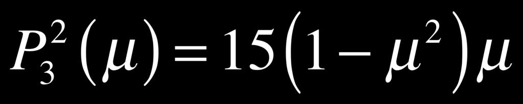
8 ! Revised April 10, :32 PM! 8 P 3 0 ( µ ) = 5 2 µ µ - - P 1 3 ( µ ) = µ 2 µ P 3 2 ( µ ) = 15( 1 µ 2 )µ

9 ! Revised April 10, :32 PM! P 3 3 ( µ ) = 15 1 µ 2 ( 1 µ 2 ) It can be shown that the associated Legendre functions are mutually orthogonal, i.e., 1 1 P m n ( µ ) P m l ( µ )dµ = 0, for n l, and P m 2 2 n ( µ ) ( dµ = 2n +1 n + m)!. ( n m)! 1 It follows that the functions 2n +1 ( 2 n m)! ( n + m)! P n are mutually orthonormal for 1 µ 1. m µ 1 ( ), n = m, m +1, m + 2, (18) (19) Referring back to (9), we see that a particular spherical surface harmonic can be written as Y n m ( µ,λ) = P m n ( µ )exp imλ ( ). (20) It is the product of an associated Legendre function of µ with a trigonometric function of longitude. Note that the arbitrary constant has been set to unity.

10 ! Revised April 10, :32 PM! 10 Figure 1:Examples of low-resolution spherical harmonics, mapped out onto the plane. The horizontal direction in each panel represents longitude, and the vertical direction represents latitude. The numbers in parentheses in each panel are the appropriate values of n and s, in that order. Recall that the number of nodes in the meridional direction is n s. The shading in each panel represents the sign of the field (and all signs can be flipped arbitrarily). You may think of white as negative and stippled as positive. From Washington and Parkinson (1986). Fig. 1 shows examples of spherical harmonics of low order, as mapped out onto the longitude-latitude plane. Fig. 2 gives similar diagrams for n = 5 and m = 0, 1, 2,...,5, plotted out onto stretched spheres. Fig. 3 shows some low-order spherical harmonics mapped onto threedimensional pseudo-spheres, in which the local radius of the surface of the pseudo-sphere is one plus a constant times the local value of the spherical harmonic. By using the orthogonality condition (18) for the associated Legendre functions, and also the orthogonality properties of the trigonometric functions, we can show that 1 2π P m n ( µ )exp( imλ)p m l ( µ )exp( i m λ)dµ dλ = 0 unless n = 1 and m = m. 1 0 (21)

11 ! Revised April 10, :32 PM! 11 Figure 2: Alternating patterns of positives and negatives for spherical harmonics with n = 5 and m = 0,1, From Baer (1972). The mean value over the surface of a sphere of the square of a spherical surface harmonic is given by 1 2π 1 P m 2 1 n ( µ )exp( imλ) 4π dµ dλ = ( n + m)! for s 0. 2( 2n +1) ( n m)! 1 0 For the special case m = 0, the corresponding value is 1 / ( 2n + 1). (22) For a given n, the mean values given by (22) vary greatly with m, which is inconvenient for the interpretation of data. For this reason, it is customary to use, instead of P n m µ ( ), the seminormalized associated Legendre functions, denoted by P! m n ( µ ). These functions are identical with P m n ( µ ) when m = 0. For m > 0, the semi-normalized functions are defined by

12 ! Revised April 10, :32 PM! 12! nm ( µ ) = 2 ( n m )! P m ( µ ). P ( n + m )! n (23)! The mean value over the sphere of the square of P m n ( µ ) exp (imλ ) is then ( 2n + 1), for any n 1 and m. n = 2, m = 1 n = 4, m = 2 n = 4, m = 1 n = 10, m = 1 Figure 3: Selected spherical harmonics mapped onto three-dimensional pseudo-spheres, in which the local radius of the surface of the pseudo-sphere is one plus a constant times the local value of the spherical harmonic. The spherical harmonics can be shown to form a complete orthonormal basis, and so can be used to represent an arbitrary function, F ( λ,ϕ ) of latitude and longitude: F ( λ,ϕ ) = F n Yn m ( λ,ϕ ) m m= n= m (24)

13 ! Revised April 10, :32 PM! 13 Here the Y n m are the expansion coefficients. Note that the sum over ranges over both positive and negative values, and that the sum over n is taken so that n m 0. The sums in (24) range over an infinity of terms, but in practice, of course, we have to truncate after a finite number of terms, so that (24) is replaced by F = M N ( m) F m m n Y n. m= M n= m Here the overbar reminds us that the sum is truncated. The sum over n ranges up to N m (25) ( ), which has to be specified somehow. The sum over m ranges from M to M. It can be shown that this ensures that the final result is real; this is an important result that you should prove for yourself. The choice of N ( m) fixes what is called the truncation procedure. There are two commonly used truncation procedures. The first, called rhomboidal, takes The second, called triangular, takes N ( m) = M + m. (26) N ( m) = M. Triangular truncation has the following beautiful property. In order to actually perform a spherical harmonic transform, it is necessary to adopt a spherical coordinate system ( λ,ϕ). There are of course infinitely many such systems. There is no reason in principle that the coordinates have to be chosen in the conventional way, so that the poles of the coordinate system coincide with the Earth s poles of rotation. The choice of a particular spherical coordinate system is, therefore, somewhat arbitrary. Suppose that we choose two different spherical coordinate systems (tilted with respect to one another in an arbitrary way), perform a triangularly truncated expansion in both, then plot the results. It can be shown that the two maps will be identical. This means that the arbitrary orientations of the spherical coordinate systems used had no effect whatsoever on the results obtained. The coordinate system used disappears at the end. Triangular truncation is very widely used today, in part because of this nice property. (27)

14 ! Revised April 10, :32 PM! 14 Figure 4: Demonstration of the effects of various horizontal truncations of 500 m patterns of geopotential height (m) data provided originally on a 2.5 longitude-latitude grid. From Washington and Parkinson (1986). Fig. 4 shows an example based on 500 mb height data, provided originally on a 2.5 longitude-latitude grid. The figure shows how the data look when represented by just a few spherical harmonics (top left), a few more (top right), a moderate number (bottom left) and at full 2.5 resolution. The smoothing effect of severe truncation is clearly visible. References and Bibliography Baer, F., 1972: An alternate scale representation of atmospheric energy spectra. J. Atmos. Sci., 29, Jarraud, M., and A. J. Simmons, 1983: The spectral technique. Seminar on Numerical Methods for Weather Prediction, European Centre for Medium Range Weather Prediction, Reading, England, Washington, W. M., and C. L. Parkinson, 1986: An introduction to three-dimensional climate modeling. University Science Books, Mill Valley, New York, 422 pp.