New variables in spherical geometry. David G. Dritschel. Mathematical Institute University of St Andrews.

Transcription

1 New variables in spherical geometry David G Dritschel Mathematical Institute University of St Andrews Collaborators: Ali Mohebalhojeh (Tehran St Andrews) Jemma Shipton & Robert Smith (St Andrews)

2 = 1 6 Vortex dynamics = 1 3 = Π(λ, φ, t)

3 t t t Froude number: Fr = u c 1 + h Rossby number: Ro = ζ = 1 6 = 1 3 = (a) 12 (b) 2 (c) Fr max : Ro max : Ro min : middle, bold curve upper, thin curve lower, thin curve

4 Depth anomaly, h = 1 6 = 1 3 = h = 002

5 Velocity divergence, δ/ = 1 6 = 1 3 = (0002) (0005) (0010) NB: In the time mean, δ rms ζ rms = 00373, and 00653

6 Acceleration divergence, γ/4ω 2 E = 1 6 = 1 3 = (002) (005) (010) NB: In the time mean, γ rms ζ 2 rms = 0767, 0773 and 0847

7 Acceleration, a /4Ω 2 E = 1 6 = 1 3 = (0001) (0002) (0005)

8 Meridional velocity, v, for the case = 1 3 v 0 : velocity obtained for δ = γ = 0 v v 0 v v (020) (020) (001)

9 Why another shallow-water model? Explicit potential-vorticity (PV) conservation has never been implemented in spherical geometry Wave vortex decomposition not well understood even in this simple context Accurate modelling of both the PV-controlled balanced flow and the imbalanced flow is now possible

10 The shallow-water equations Du Dt + fk u = c2 h h t + [(1 + h)u] = 0 where h (h H)/H, c 2 = gh, f = sin φ, H is the mean depth, g is gravity, and u is tangent to the sphere Dissipation and forcing terms are not included These equations may be combined to show DΠ Dt = 0, where Π = ζ + f 1 + h is the potential vorticity (PV) NB: ζ = k ( u)

11 New variables The original equations hide PV conservation numerically, PV is poorly conserved The distribution of PV largely controls the fluid motion (u, h) through hidden balance relations (PV inversion) Hoskins, McIntyre & Robertson (1985), McIntyre & Norton (1999), Ford, McIntyre & Norton (2000), etc numerically, a poor representation of the PV leads to a poor representation of the fluid motion The residual motion, the imbalance (gravity waves), may be prone to large errors

12 Two distinct types of motion co-exist: Slow balanced vortical motions, and Relatively fast imbalanced wave motions which however are deeply intertwined

13

14 A new approach Enforce PV conservation explicitly (preserve its advective character) use contour advection; Distinguish the PV-controlled balanced motions and the residual imbalanced motions, at least to leading order use imbalanced prognostic variables Dritschel & Mohebalhojeh (2000), M & D (2000,2001,2004), D & Viúdez (2003), V & D (2003,2004)

15 Explicit PV conservation A particle representation for PV is natural: each particle x = X conserves its value of Π DΠ Dt = 0 dx dt = u(x, t) A contour representation is even more natural, since exchanging any pair of particles on a contour Π = constant does not alter the distribution of Π

16 Numerics: an ideal algorithm? The Contour-Advective Semi-Lagrangian (CASL) algorithm (Dritschel & Ambaum, 1997) makes direct use of this contour representation, and deals with the non-locality (inversion) efficiently It represents the PV by a finite set of contours the Lagrangian aspect represents the velocity by fixed grid points the Eulerian aspect and provides efficient means of communication between the two representations interpolation, and its inverse, filling

17 Each PV contour is represented by nodes, connected together by cubic splines Shown also is the underlying grid Note that Π is permitted to have much finer structure than u This exploits the fact that u is typically a smoother field than Π

18 Balance relations Having chosen the PV as one prognostic variable, what is a sensible (accurate and convenient) choice for the other two? In a balanced model, the fluid motion (u b, h b ) is fully controlled by the PV The balanced motion is recovered by PV inversion, ie by solving equations of the form F(u b, h b ) = 0, G(u b, h b ) = 0, H(u b, h b ) = 0 for u b and h b, given the PV Π One of these equations comes from the definition of PV: F = k ( u b ) + f Π(1 + h b ) = 0 The other two come from imposing particular relations between variables, eg as in geostrophic balance

19 For example, one may set two successive time derivatives of the divergence δ = u to be zero, ie G = δ (n) = 0, H = δ (n+1) = 0 generating the δ hierarchy The forms of G and H are found by recursively substituting the original equations (M & D 2001) Another example, used here, sets G = δ (n) = 0, H = γ (n) = 0 where γ = a and a = Du/Dt NB: a = fk u c 2 h It makes sense that the new variables should represent what the PV cannot The new variables could be G and H themselves

20 Here, we use the simplest member, n = 0, of the δ-γ hierarchy In other words, we take G = δ, H = γ to be the other two prognostic variables On the f-plane, γ is proportional the ageostrophic vorticity, ζ c 2 2 h/f Setting γ = δ = 0 then leads to geostrophic balance (cf M & D 2001) The variables γ and δ thus represent the departure from geostrophic balance On the sphere, γ = fζ βu c 2 2 h where β = df/dφ = cos φ and u is the zonal velocity component

21 The prognostic equations for δ and γ are δ t = γ u 2 2 (δu) [ u φ ( ) u φ + ζ + v φ ( )] v φ δ γ t = c 2 2 { [(1 + h)u]} + B λ (Zu) where B c 2 h 1 2 u 2 (Bernoulli pressure), Z = f(ζ + f), and λ is longitude However, the tendencies involve the original variables u and h These are recovered by a kind of PV inversion analogous to what is done in a balanced model

22 Inversion Inversion here simply means finding u and h from the prognostic variable set (δ, γ, Π) This is accomplished as follows Let u = k ψ + χ then the potentials satisfy 2 ψ = ζ & 2 χ = δ But ζ depends on h through the definition of PV: ζ = (1 + h)π f So, we need to find h before we can invert ζ But the definition of γ implies c 2 2 h fπ h = f(π f) βu γ, using ζ above

23 While the inversion equations are coupled, they are linear, an exceptional property Numerically, they are solved iteratively and convergence is exponentially fast Solve 2 χ = δ first u χ Then iteratively solve 2 ψ n+1 = ζ n = (1 + h n )Π f u n+1 and (c 2 2 f 2 ) h n+1 = f(ζ n f h n ) βu n+1 γ ψ n+1 and h n+1

24 n Numerics All fields represented on a regular lat-lon grid, with φ = λ/2 (n φ = n λ ) Semi-spectral approach: advantageous for inverting c 2 2 f 2 (tridiagonal procedure) 2 nd -order finite differences in φ Semi-implicit time stepping, but t < t CFL = φ/c Minimal Robert-Asselin filtering: A = c t 2/3 spectral filter applied to nonlinear parts of δ & γ tendencies: m/ cos φ λ /2 (D & V 2003)

25 Verification Standard Rossby-Haurwitz wave test and a perturbed variation (cf Thuburn & Li 2000) t = 0 t = 5 Π (06) h (002) 022% energy variation over 5 days 031% angular momentum variation Note : n φ = n λ = 128 Usual spatial and temporal resolution variations

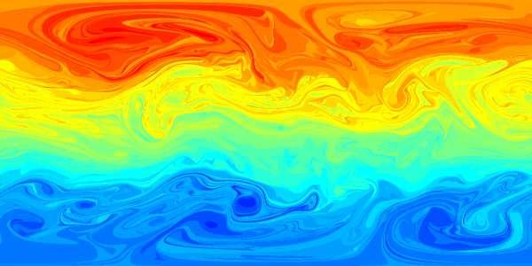
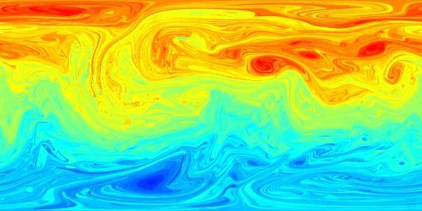
26 An application to turbulence Random PV anomaly ϖ = Π f spatially correlated over a length L c = 1/10 ϖ, polar view ϖ, equatorial view Prescribed mean Rossby radius L R = c/ = 1/3 Planetary rotation Ω E = 2π n φ = n λ = 128, t = 0004 ( t CFL = 00058)

27 Initialisation (V & D 2003, D & V 2003) Generate initial fields of δ and γ ( u and h) by ramping up the PV anomaly ϖ from 0 to its desired amplitude over a period τ I 1: 1 T (τ) 0 0 τ I τ Meanwhile, evolve δ and γ using the full model, and advect the PV contours δ = γ = u = h = 0 at τ = 0 NB: the PV jump across each contour increases like T (τ) The state at τ = τ I is considered the initial state, t = 0

28 PV contours at τ = 0 PV contours at τ = τ I φ λ Note, Π = f on the left since T (0) = 0 Here τ I = 20 days in three cases: = 1 6, 1 3, and 1 2

29 Gravity waves It is common to call the residual imbalance gravity waves, but this can be misleading The balanced flow can be defined in many ways We could make use of the balance hierarchies such as δ (n) = γ (n) = 0, but they prove ineffective for highly nonlinear flows A new alternative, called the Optimal PV (OPV) balance (V & D 2004), is to define the PV-controlled balanced flow as the flow which evolves into the current PV distribution after a long ramp period τ D

30 That is, we seek the base configuration X base of PV contours, at a time t τ D, which evolves into the current PV contours X while ramping up the PV as in initialisation from a state of no motion t τ D t φ λ The fields of h, δ, γ, etc at the end of this ramped evolution are called the balanced fields, h b, δ b, γ b, etc

31 In practice, X base and hence h b, δ b, γ b, etc are found iteratively in a cycle of forward and backward integrations (V & D 2004) X Π X b Π b X base h b h resid 0 0 τ D τ h b, δ b, γ b, etc depend only on Π and τ D The imbalanced fields are h i h h b, δ i δ δ b, γ i γ γ b, etc

32 Convergence h i rms / h rms (a) 03 δ i rms /δ rms (b) τ D τ D γ i rms /γ rms (c) 003 u i rms / u rms (d) τ D τ D 1 st -order δ γ balance is plotted along τ D = 0

33 Comparison Balance h i rms h rms δ i rms δ rms γ i rms γ rms u i rms u rms δ = γ = δ t = γ t = OPV, τ D = All results are for = 1 3

34 Imbalanced depth h i δ = γ = 0 at t = 5 for = 1 3 δ t = γ t = 0 OPV, τ D = 2 OPV, τ D = 3 OPV, τ D = 4 OPV, τ D = 5 h = except for δ = γ = 0 balance for which h = 0005

35 Velocity divergence δ/ at t = 5 = 1 6 = 1 3 = 1 2 δ δ b δ i (0002, 00002) (0005, 0001) (0010, 0005) NB: All results are henceforth for τ D = 5

36 Imbalanced depth anomaly, h i = 1 6 = 1 3 = (000005) (00005) (0005)

37 Imbalanced velocity divergence, δ i / = 1 6 = 1 3 = (00002) (0001) (0005)

38 Imbalanced acceleration divergence, γ i /4Ω 2 E = 1 6 = 1 3 = (0002) (001) (005)

39 Frequency spectra h 10 2 δ = ω ω = ω 1 10 ω = ω ω

40 Finalé Greater accuracy can be achieved by explicitly distinguishing the vortical and the wave components of a flow Gravity waves are more clearly identified when taking full account of the flow inertia, as in the OPV balance procedure Similar results have been found for both spherical shallow-water flows and for three-dimensional non-hydrostatic flows