Self-adjustment of stream bed roughness and flow velocity in a steep

Transcription

1 Self-adjustment of stream bed roughness and flow velocity in a steep mountain channel AUTHORS Johannes M. Schneider 1,2, johannes.schneider@usys.ethz.ch (corresponding author) Dieter Rickenmann 2, dieter.rickenmann@wsl.ch Jens M. Turowski 2,3, turowski@gfz-potsdam.de James W. Kirchner 1,2, kirchner@ethz.ch 1) Department of Environmental Systems Science, ETH Zurich, Zürich, Switzerland 2) Mountain Hydrology and Mass Movements, Swiss Federal Research Institute WSL, Birmensdorf, Switzerland, 3) Helmholtz Centre Potsdam, GFZ German Research Centre for Geosciences, Potsdam, Germany Abstract Understanding how channel bed morphology affects flow conditions (and vice versa) is important for a wide range of fluvial processes and practical applications. We investigated interactions between bed roughness and flow velocity in a steep, glacier-fed mountain stream (Riedbach, Ct. Valais, Switzerland) with almost flume-like boundary conditions. Bed gradient increases along the 1-km study reach by roughly one order of magnitude (S=3-41%), with a corresponding increase in streambed roughness, while flow discharge and width remain approximately constant due to the glacial runoff regime. Streambed roughness was characterized by semi-variograms and standard deviations of point clouds derived from terrestrial laser scanning. Reach-averaged flow velocity was derived from dye tracer 1 This article has been accepted for publication and undergone full peer review but has not been through the copyediting, typesetting, pagination and proofreading process which may lead to differences between this version and the Version of Record. Please cite this article as an Accepted Article, doi: /2015WR016934

2 breakthrough curves measured by 10 fluorometers installed along the channel. Commonly used flow resistance approaches (Darcy-Weisbach equation and dimensionless hydraulic geometry) were used to relate the measured bulk velocity to bed characteristics. As a roughness measure, D 84 yielded comparable results to more laborious measures derived from point clouds. Flow resistance behavior across this large range of steep slopes agreed with patterns established in previous studies for both lower-gradient and steep reaches, regardless of which roughness measures were used. We linked empirical critical shear stress approaches to the variable power equation for flow resistance to investigate the change of bed roughness with channel slope. The predicted increase in D 84 with increasing channel slope was in good agreement with field observations. Keywords Mountain stream, bed roughness, flow resistance, flow velocity, point cloud, semi-variogram, dye tracer, critical shear stress Key points D 84 is similar to point cloud roughness parameters Flow resistance equations for shallow streams also apply in very steep channels Critical stress approaches are able to predict bed adjustment to bed slope and water flow 2

3 1. Introduction Flow velocity is an essential determinant of many fluvial processes and properties, including flood routing, transport of nutrients, pollutants, and sediments, and aquatic habitat quality. However, despite decades of research it is not fully understood how flow velocity is controlled in gravel-bed streams, especially in steep mountain channels where the bed morphology is typically complex and rough. As bed gradients steepen, flow resistance typically rises due to the increasing proportion of coarse roughness elements such as immobile boulders, bedrock constrictions or large woody debris. Furthermore, flow resistance strongly increases with decreasing relative submergence, i.e. the ratio of flow depth to a characteristic roughness size [Bathurst, 1985; Ferguson, 2010; Lee and Ferguson, 2002; Limerinos, 1970; Reid and Hickin, 2008; Wilcox and Wohl, 2006]. Grain, form and spill resistance are all important in steep streams. Whereas grain resistance is related to the skin friction and form drag on individual grains on the stream bed surface [Einstein and Barbarossa, 1952], form resistance is related to the pressure drag on irregular bed surfaces [Leopold et al., 1995]. Spill resistance in step-pool or cascade streams [Montgomery and Buffington, 1997] results from turbulence when supercritical flow decelerates as fast flows meet slower-moving water [Leopold et al., 1995; Leopold et al., 1960; Wilcox et al., 2006]. Spill resistance is typically dominant in step-pool or cascade mountain streams [Abrahams et al., 1995; Comiti et al., 2009; Curran and Wohl, 2003; David, 2011; Wilcox et al., 2006; Zimmermann, 2010] and generally decreases with increasing flow stage [David, 2011; Wilcox et al., 2006]. Flow resistance relations may be used to predict flow velocity in steep streams where no direct measurements are available. Flow resistance calculations are typically based on the Manning or Darcy-Weisbach equations (Equation (1)), 3

4 1/2 2/3 S d 8gdS v n f tot 1 where n is the Manning coefficient, f tot is the Darcy-Weisbach friction factor, S is the energy slope (in this study S is approximated by the channel bed slope), d is the hydraulic radius (or flow depth) and g is gravitational acceleration [m s -2 ]. Many studies have identified relations between measures of roughness height R (e.g., D 84 ) and bed or flow characteristics; comprehensive overviews of flow velocity predictions based on n or f tot can be found in Powell [2014], Rickenmann and Recking [2011], and Yochum et al. [2012]. In particular, low submergence of roughness elements (i.e. small relative flow depth d/r), typical for steep streams, was determined to be an important agent for flow resistance [e.g., Aberle and Smart; 2003; David et al., 2010; Ferguson, 2010; Recking et al., 2008; Wohl and Merritt, 2008; Wohl et al., 1997; Yochum et al., 2012]. Alternatively, hydraulic geometry relations have been scaled and non-dimensionalized using a roughness height R [Ferguson, 2007] and channel bed slope [Nitsche et al., 2012; Rickenmann and Recking, 2011] to account for the increased influence of macro-roughness elements on flow velocity when flows are steep (Equations (2) and (3)). v** v gsr 2 q q** 3 3 gsr Here v** is the dimensionless velocity and q** the dimensionless discharge. These quantitative methods generally provide better estimates of (dimensional) flow velocities in steep streams than approaches using scaled flow depth and f tot do [e.g., Comiti et al., 2009; Nitsche et al., 2012; Rickenmann and Recking, 2011; Zimmermann, 2010]. One reason for this finding is the difficulty of measuring or defining representative flow depths in steep streams with irregular bed forms [Rickenmann and Recking, 2011]. 4

5 When relating flow stage, flow velocity, discharge or resistance to bed characteristics (e.g. using the Darcy-Weisbach or the dimensionless hydraulic geometry equations), the D 84 of the streambed surface layer is often selected as dominant roughness height R [Aberle and Smart, 2003; Comiti et al., 2009; Comiti et al., 2007; Ferguson, 2007; Zimmermann, 2010]. Other roughness measures to characterize (additional) flow resistance have also been proposed, including boulder concentration [Pagliara and Chiavaccini, 2006; Whittaker et al., 1988], boulder protrusion [Yager et al., 2007] or step height and spacing [Egashira and Ashida, 1991]. It is still an open question which roughness measure is most representative for flow resistance in steep and rough streams, considering that natural beds are composed of heterogeneously sized grains which are non-uniformly spaced and protrude into the flow to varying extents [Kirchner et al., 1990]. Field estimates of a characteristic grain size such as D 84 are often associated with large uncertainties due to operational bias [Marcus et al., 1995; Wohl et al., 1996], limited sample size [Church et al., 1987; Milan et al., 1999], incompatibility between sampling methods [Diplas and Sutherland, 1988; Fraccarollo and Marion, 1995] and spatially heterogeneous grain size distributions [Buffington and Montgomery, 1999; Crowder and Diplas, 1997]. With the further development of photogrammetry and laser scanning technologies, there are new possibilities for obtaining detailed topographic information and streambed roughness measures, including the standard deviation, semi-variance, skewness or kurtosis of the bed surface elevations [e.g., Heritage and Milan, 2009; Rychkov et al., 2012; Smart et al., 2002; Yochum et al., 2012]. Previously introduced approaches often consider bed roughness measured at a given moment as a constant parameter over time. Considering a stream as a self-organized system with feedback mechanisms between bed morphology, hydraulics and sediment transport, it may be assumed that bed roughness adjusts to bed gradient and flow conditions, reflecting the dominant hydraulic stresses that were responsible for the formation of the streambed. It is 5

6 commonly argued that the bed adjusts to maximize flow resistance [e.g., Davies and Sutherland, 1980; Davies and Sutherland, 1983] because maximum flow resistance is connected with maximum bed stability [Abrahams et al., 1995]. Bed stability and bed adjustment are closely related to the grain sizes that can be entrained under specified bed gradients and flow conditions. A commonly used parameter that describes critical conditions of particle entrainment is the critical shear stress τ* c, which incorporates in its dimensionless form a critical flow depth d c, the bed gradient S and the related grain size D x (Equation (4)), * ds c c 4 ( s 1) DX where s is the relative density of the sediment (s 2.65). In a simplified assumption, the critical shear stress controls bedload entrainment, or even debris-flow formation at very steep slopes [Prancevic et al., 2014] and thus the bed composition and stability. Typically, bed stability is increased at steeper slopes and thus positive correlations of the critical shear stress with bed slope were identified in several studies [e.g., Bunte et al., 2013; Camenen, 2012; Ferguson, 2012; Lamb et al., 2008; Prancevic et al., 2014; Recking, 2009; Shvidchenko et al., 2001]. These positive correlations of τ* c against bed slope are mainly explained by increased bed stability at steep slopes due to interlocking of bed particles [Church et al., 1998], variable friction angles, flow aeration (lower water density) and increased turbulent conditions [Lamb et al., 2008]. However, in addition to the ratio between the available shear stress and the critical shear stress, there are other important factors in steep and narrow streams with a pronounced step-pool morphology: for example, the jamming of large particles, and thus the stability of steps, depends also on the sediment concentration in the flow and on the ratio of stream width to grain diameter [Church and Zimmermann, 2007]. Here we study a steep, glacier-fed mountain stream with almost flume-like boundary conditions. Along the channel, the bed gradient (S) and roughness (here D 84 ) both 6

7 systematically increase by roughly an order of magnitude (with S = % and D 84 = m, respectively), while channel width and flow discharge remain approximately constant in the downstream direction during the summer period, which has the largest glacier meltwater runoff. We compiled a detailed dataset of bed characteristics (e.g., grain size distributions, bed topography) and flow velocities measured at different flow discharges. Based on these field data, we evaluated how well flow resistance equations and hydraulic geometry relations predict flow velocity at bed slopes up to 40% (whereas previous field data have been generally limited to slopes <25%). We also compared different roughness measures for scaling flow depth and hydraulic geometry relations, using D 84 and terrestrial laser scanning (TLS) point cloud statistics such as the standard deviation, the semi-variance or inter-percentile ranges of bed elevations. Finally, we tested how bed roughness should adjust to bed slope and driving hydraulic forces, by combining the variable power flow resistance equation [Ferguson, 2007] with recently derived empirical critical shear stress approaches [Camenen, 2012; Lamb et al., 2008] and comparing the results with measured bed characteristics. 2. Data and Methods 2.1. Study Site The Riedbach is an alpine, glacier-fed stream located in the Matterhorn valley close to St. Niklaus (Figure 1). The Riedbach flows with a slightly meandering path over the glacier forefield with bed gradients ranging from about 2.8 to 6% before reaching a knickpoint and plunging into a very steep reach with gradients of up to 41% (Figures 2 and 3). In this stretch of the channel, the Kraftwerke Mattmark AG (KWM) operates a water intake for hydropower generation, which forms the lower limit of the 1-km stream section that we studied. At the 7

8 water intake, the Riedbach drains a watershed of 15.8 km 2, of which 53 % is glacier-covered (as of 2001; Vector swisstopo (DV033594)). The catchment elevation range is m a.s.l. The runoff regime is dominated by snow and glacial melt during early and mid-summer. In this season, daily peak discharges between 2 m 3 s -1 and 4.5 m 3 s -1 are reached during about 50 days each year (Figure S1, supporting information). Maximum discharges during intense summer rainfalls are unmeasured, but can be roughly quantified here from specific peak flows of comparable mountain catchments in the Valais and southern Switzerland. In these catchments the mean annual specific peak flow discharges are about 0.5 m 3 km -2 s -1 with maximum values recorded ranging between 1 and 1.5 m 3 km -2 s -1 during the last 50 years [Weingartner et al., 2014]. If similar specific peak flows characterize the Riedbach, they would correspond to discharges of roughly 8-24 m 3 s -1. Bedload transport is monitored in the Riedbach using the indirect Swiss plate geophone system [e.g. Rickenmann et al., 2014] installed at the water intake downstream of the steep stream section (Figure 1). The geophone plates continuously register the impacts of moving stones and thus indirectly measure bedload transport intensities. The continuous bedload transport measurements indicate that transport primarily occurs in summer when flow discharge rates are high due to glacial meltwater. During the 6-year period that these geophone sensors have been in operation ( ), no debris flows were recorded in the main channel, suggesting that sediment transport in the Riedbach is predominantly characterized by fluvial erosion and transport. There is clear visual evidence of high sediment availability in the recent glacier retreat area, about 1 km above the beginning of study section. Here, the glacier retreated by roughly 600 m since 2008 (including 500 m in 2008 alone) [Glaciological Reports , VAW/ETHZ & EKK/SCNAT (2015), and left a large dead ice body 8

9 covered by a thick sediment layer that supplies sediment when the dead ice melts. However, within the studied stream section, sediment availability and sediment supply appear to be low. The first reach of the studied stream section was deglaciated roughly 50 years ago (the glacier snout was roughly at the location of the first study reach from 1895 to 1960) [Glaciological Reports , VAW/ETHZ & EKK/SCNAT (2015), In the decades since deglaciation, a vegetation cover has already developed. Furthermore the banks are characterized by low gradients (Figure 2a and b), so significant sediment supply from bank erosion or the lateral moraines is unlikely. In the steep reach, the banks are mainly characterized by exposed bedrock (on the orographic left hand side of the channel) or dense vegetation (Figure 2d). There is only one tributary with regular debris-flow activity along the study reach; however its confluence is located immediately upstream of the water intake (on the orographic right hand side of the channel), and thus it does not influence the grain size distribution along the channel bed in the study section. For this study we defined channel reaches with more-or-less homogeneous bed gradients and bed morphologies, for which the bed characteristics (grain size distributions, bed topography) and the flow velocity and other hydraulic parameters were determined. At the upstream and downstream end of each reach, a fluorometer was installed for dye tracer studies. Study reaches and fluorometer locations were numbered as, for example, R#01 and Fl#01 respectively (Table 1) Characteristic grain sizes and roughness density Grain size distributions were determined using the line-by-number (LBN) method [Fehr, 1987], consisting of (median 380) counts of individual particles within each sampled reach. The characteristic grain sizes D 30, D 50, and D 84 coarsen significantly along the 9

10 stream with increasing bed gradients from about 0.05/0.09/0.21 m to 0.2/0.43/1.18 m (Table 1). In addition, a grid-by-number pebble count (PC) was taken on the glacier forefield for R#01 [Bunte et al., 2013]. Full grain size distributions are given in the supporting information (Figure S3). Roughness density was characterized using the boulder concentration λ=n b πd 2 b /(4A b ), where n b is the number of boulders, D b is their mean diameter, and A b is the sampled area. As a simple assumption a fixed critical diameter of 0.5 m was used to define an immobile boulder [cf. Nitsche et al., 2012], instead of using a critical diameter that depended on flow stage and bed gradient Bed topography The streambed surface was surveyed with a terrestrial laser scanner (ScanStation C10, Leica Geosystems AG, Heerbrugg, CH) during autumn low-flow conditions. We scanned representative reaches in (i) the glacier forefield with a 2.8% bed gradient (corresponding to the 50 m long Reach R#01), (ii) the transitional reaches with bed gradients from 6% to 42% (350 m long, Reaches R#03 to R#07), and (iii) the steep, downstream end of the study section with a bed gradient of 38% (100 m long, Reach R#10) (see thick black lines in Figure 3). In total, we scanned from about 30 different positions resulting in an average point cloud density of about 5 points/cm 2, with a mean absolute registration error of 3 mm. Due to the very rough bed topography in the steep reach, shadow effects could not be avoided (Figure 4). Cross-sectional profiles were derived from the TLS point cloud at 0.2 m intervals along the longitudinal profile for reaches R#01, R#03-R#07 and R#10. Cross-sectional profiles for reaches R#02 and R#08 (5 cross sections each) were recorded using a total station and a laser distance meter, respectively. 10

11 From the complete point cloud, individual patches representing the local bed topography were exported for further statistical analysis (Table 1). The analyzed patches were defined according to the following criteria: no banks, as little missing data due to shading and water cover as possible, a representative area as large as possible, no large-scale structures (e.g., concave or convex forms, coves or notches), and a minimum width twice the largest grain size within each reach. The analyzed patches were typically rectangular with two of their sides parallel to the flow direction. The noise within the point cloud was reduced and outliers were removed using Geomagic Studio 2014 (3D Systems, Rock Hill, SC, USA, 2014). The point cloud density was equally spaced and limited to not exceed 4 points/cm 2. Finally, the patches were de-trended for local slope. As a measure of bed roughness for each analyzed patch, we calculated the 90% interpercentile range (IPR 90 ) defined by the 95 th percentile minus the 5 th percentile of all detrended elevation values. Furthermore, we calculated the standard deviation STD z (see also Brasington et al. [2012]) and the semi-variogram [Hodge et al., 2009; Robert, 1988; 1991] using the de-trended elevations. For each patch within a reach with a characteristic bed gradient (R#01-R#10), the surface statistics (IPR 90, the semi-variogram sill values, and the standard deviation STD z ) of the TLS point cloud were averaged (median), and the variability between patches was characterized by the inter-patch standard deviation (note, this standard deviation is different from STD z ; Table 1). In addition, the point cloud was interpolated onto a regular grid and the roughness parameters (the inter-percentile range, the standard deviation and the semi-variogram) were re-calculated based on the gridded data. This was done to further quantify the uncertainties in the roughness measures, whether derived from the point cloud or gridded data. 11

12 Semi-variance The semi-variance is a commonly used statistic to characterize spatial correlations of vertical distances at increasing lags, and it is defined as half the variance at lag h (Equation (5)). 1 2 Nh ( ) 2 5 (, i j) N h h zi zj Here, N is the number of elements (within lag h) and z is the vertical elevation. The semivariance of a gravel-bed river typically increases with increasing lag distance until it reaches a more-or-less constant level (the sill ) at some lag distance (the range ). To determine the range and sill values we fitted a simple spherical model (Equation (6); see Figure S4 supporting information) to the isotropic semi-variogram: h 3 3 h 1h cn cp if 0 h r 2 r 2 r 6 cn cp if h r Where r is the range, c p is the partial sill value and c n is the nugget (defined here as the semivariance at the smallest lag-distance). The total sill value is defined in this study as c=c p +c n. For computational reasons, the semi-variogram was usually calculated on points. In preliminary tests it could be shown that including additional points did not increase the quality of the semi-variogram. The minimum lag distance was 0.01 m and the maximum lag was defined as half the width of the analyzed patch. Because the sill value c is related to the semi-variance, and variance is the square of the standard deviation, we multiplied c by two and took the square root c' 2c to compare the sill with the other roughness measures, such as the characteristic grain sizes, inter-percentile ranges and standard deviation. 12

13 2.4. Flow discharge Flow discharge rates Q WI were gauged in 10-minute sampling intervals in the settling basin of the water intake. Water that bypasses or overtops the water intake is not measured. We apply a correction factor of 1.2, estimated from dye tracer dilution measurements (see Text S2, supporting information), to correct for the unmeasured component of streamflow. Throughout this study, flow discharge rates Q refer to these corrected values. The capacity of the water intake is about 4 m 3 s -1 (or roughly 4.8 m 3 s -1 with the correction factor), and measurements of higher flows are not available. We assume discharge rates are constant along the 1 km studied stream section, because streamflow is dominated by glacier melt and no significant rainfall events occurred during the field measurements. We also assume that there was no substantial groundwater contribution to the stream, because the catchment area only increases by a factor of 1.1 over the studied stream section and the local geology is dominated by relatively impermeable crystalline rocks Reach averaged hydraulic parameters Flow velocity (measured) We conducted 46 dye tracer experiments at the Riedbach during the summer and autumn of In-situ fluorometers (GGUN-FL30, Albillia SA; Schnegg [2003]) were installed at ten locations from the glacier forefield to the water intake. These locations were selected to define reaches with relatively homogeneous bed gradients and bed morphologies between pairs of fluorometers (Figure 3, Table 1). The fluorometers were installed as far as possible (typically around 1 m) from the banks. It was not possible to install the fluorometers in the middle of the stream during high flows. Dye tracer (fluorescein) was either injected on the 13

14 glacier forefield at injection location Inj#01, 92 m upstream of the first fluorometer Fl#01, or near the transition to the steep reaches, at injection location Inj#02, 43 m upstream of Fl#05. The tracer was injected by splashing a bucket of diluted dye as evenly as possible across the width of the channel. The raw fluorometer data (mv) were calibrated against reference dye concentrations (ppb), and measured background values were leveled to zero before each injection. The beginning of each individual breakthrough curve (BTC) was determined visually. The end of the BTC was defined as the point where 99% of the tracer had passed the fluorometer. Outliers within the BTCs were removed using a robust spline filter. For each BTC the concentration-weighted harmonic mean was determined to derive the mean travel time and flow velocities [Waldon, 2004]. The reach-averaged flow velocity was determined by scaling the distance by the (harmonic) mean travel times between two fluorometers. To increase the database for further analysis, we considered not only reaches between two adjacent fluorometers, but also some reaches between all pairs of fluorometers (Table 1) that share similar bed slope and bed topography (Dataset S1 in the supporting information includes the flow velocity data) Flow width, depth, and hydraulic radius (back-calculated) Hydraulic parameters including flow area (A), flow width (w), wetted perimeter (w p ), flow depth (d h =A/w) and hydraulic radius (d=a/w p ) were back-calculated from the reach-averaged flow velocity (v) for each cross-sectional profile (derived as described in section 2.3) using the continuity equation (A=Q/v). Note, flow depth in all calculations and figures is approximated with the hydraulic radius d, consistent with the conventional practice in narrow channels. The hydraulic parameters were then averaged over the available cross-sections within each reach. Averaging the hydraulic parameters rather than the available cross-sections themselves (as done by Nitsche et al. [2012]) was preferred due to the rough bed topography, 14

15 including large boulders, which made it difficult to derive averaged cross-sections. Note that hydraulic parameters were back-calculated as reach averages and thus neglect potential waterair mixtures Uncertainties in the hydraulic variables Uncertainties in the flow velocity (v) measurements might originate from sunlight degradation of the fluorescein tracer or from incomplete tracer mixing. Typical fluorescein degradation by sunlight is estimated as 5% or less for low-flow conditions and 2% or less for high-flow conditions (assuming bright sunlight, a degradation half-life of 10 hours, e.g. Leibundgut et al., [2009], and travel times of roughly 60 minutes and 20 minutes, for low and high flows, respectively). By modeling these degradation effects on a typical breakthrough curve during low flow conditions with the longest travel times, we calculate that they alter the harmonic mean estimate (which the flow velocity is derived from) by only 0.1 % or less. Uncertainties in v due to incomplete dye tracer mixing were estimated by installing two fluorometers at the left and right banks of individual cross-sections. These fluorometer pairs yielded velocity estimates that agreed within 13% during moderate flows at the first crosssection downstream of each injection location (Inj#01 and Inj#02), and 1-5% during low flows at the second fluorometer cross-section downstream of each injection location (with presumably smaller discrepancies farther downstream). Typical flow velocity uncertainties are therefore estimated at a few percent. This inference is supported by the very strong relationship between v and (independently measured) Q, with high correlation coefficients and small standard errors for all of the considered reaches (Table 2). Uncertainties in the back-calculated hydraulic variables arise from both the flow velocities and from the measured cross-sections. For example, the cross-sections measured by TLS every 0.2 m, as described in section 2.3 above, yield hydraulic radii with a standard deviation 15

16 of 10-11% in reach R#01 on the glacier forefield and 25-46% in steep reach R#10 (where the given ranges characterize high and low flows, respectively). From these measurements, and accounting for their spatial autocorrelation, we estimate the standard error in the mean hydraulic radius at roughly 3-5% for glacial forefield reaches like R#01, and 5-15% for steep reaches like R#10. These estimates can be checked by comparing the hydraulic parameters estimated from total station cross-sections and TLS-derived cross-sections for reaches R#05 (4 crosssections) and R#10 (5 cross-sections), where both measurements are available. The resulting hydraulic parameters correspond almost exactly to one another in R#05 and differ by about 20% in the steeper and rougher reach R#10, broadly consistent with the uncertainty estimates derived above Streambed adjustment to hydraulic conditions To mechanistically explore how increasing bed gradients affect bed roughness, we use two different measures of the bed-forming discharge in each channel reach: a) the bankfull flow, as defined by the bank height in the glacier forefield and the lower limit of perennial vegetation in the steep reaches; see Williams [1978], and b) the effective discharge, as defined by the magnitude and frequency of the bedload transport intensities [e.g. Andrews, 1980; Downs et al., 2015; Soar and Thorne, 2013; Wolman and Miller, 1960], determined here based on the geophone measurements at the water intake (see section 2.1). We then used the variable power flow resistance equation (VPE) of Ferguson [2007] (Equation (A1)) combined with two different critical shear stress approaches to solve for the critical grain diameter D 84 that can be transported by either of the two bed-forming discharges described above. The detailed derivation and the resulting equation to estimate D 84 as a function of bed slope can be found in Appendix A. The critical shear stress approaches considered are the widely cited 16

17 Lamb et al. [2008, Fig. 1] equation (Equation (7)), and the approach of Camenen [2012, Eq. (9)] (Equation (8) here, assuming τ* c0 =0.05 and an angle of repose φ s of 50 ) based on experimental data of Recking [2009] and a study of Parker et al. [2011]. * 0.25 c 0.15S 7 S * * sin( s arctan ) c co S 8 sin( s ) For the sake of completeness, we also considered the recent critical shear stress approaches of Bunte et al., [2013, Fig. 4] and Recking [2009, Eq. (23)] and the reference shear stress approaches of Mueller et al. [2005, Eq. (6)] and Schneider et al. [2015, Eq. (9)], however these approaches deviated significantly from the observations, and are shown only in the supporting information. Because the critical shear stress approaches presented here refer to a D 50 rather than D 84, the equations were modified assuming a factor of δ = D 84 /D 50 =2.6 (see Appendix, Equation (A5)), corresponding to the average D 84 /D 50 ratio measured in the Riedbach. Using a value of δ = 2.6 assumes that no hiding and exposure effects would ease particle entrainment for the D 84 size class compared to the D 50 size class. To account for potential hiding effects [Parker, 2008], the hiding function of Wilcock and Crowe [2003] was used, with b = (0.67/1+exp( )) = 0.503, giving * c84 /* c50 = (D 84 /D 50 ) b-1 = for D 84 /D 50 = 2.6, resulting in a reduced factor δ = = Results 3.1. The channel bed morphology With increasing bed gradients, a dramatic increase in the bed's grain size diameter and topographic irregularity can be observed. All measures of bed roughness show strong positive correlations with bed slope, with power-law slopes around 0.75 (Figure 5a). Power-law 17

18 equations in the form of Y=aX b, r 2 values, and residuals are based on linear regression analysis on log-transformed values throughout this study, unless otherwise noted. Whereas the inter-percentile range IPR 90 is similar to D 84, the sill value c and the STD z are similar to D 50. The characteristic grain sizes D 50 and D 84 from reaches with shallow bed gradients (<6% bed slope; data points indicated by blue circles in Figure 5) deviate from the trend for bed gradients steeper than 6%, so the power laws were fitted for the steep reaches (>6%) only. Also, the characteristic grain sizes in reach R#01 derived from pebble counts by Bunte et al. [2013] are smaller than the characteristic grain sizes derived from line-by-number samples (Figure 5) (for more details on these observations see section 4.1). Deviations between the roughness measures derived directly from the point cloud and those derived from the roughness measured derived from interpolated, gridded data, are less than 3% for the STD z, 3% for the IPR 90 and 17% for the sill value c (Figure S5) Flow velocity, depth and width related to bed slope Measured flow velocities of all reaches obey clear power-law relationships with measured flow discharge (r ; Table 2). Flow velocity is slightly higher on the glacier forefield (at bed slopes shallower than 6%) than it is in the steeper reaches (6%), for which flow velocity is nearly constant with increasing gradient, as shown in Figure 6a for 0.5, 1.0, 2.0, and 3.0 m 3 s -1 total discharge. Flow depth and width are back-calculated from reach-averaged velocity and the cross-sectional profiles, and show no clear trends with increasing bed slope (Figure 6b and 6c). The smaller flow width in reach R#01 compared to R#02 and R#03 on the glacier forefield corresponds to field observations of a relatively narrow channel at this reach. Unit discharge rates q=q/w (m 3 s -1 m -1 ) were determined for each reach and each dye tracer experiment based on the flow width relation w=aq b (Table S1, supporting information). Flow velocity for unit discharges of 0.1, 0.2, 0.3 and 0.4 m 3 s -1 m -1 (corresponding roughly to 0.5, 18

19 1.0, 2.0, and 3.0 m 3 s -1 total discharge) is generally highest on the glacier forefield at bed slopes of S=3-12% and somewhat smaller for the steeper reaches with S 12% (Figure 6d). The uncertainties in the velocity and the related hydraulic parameters (calculated as described in section 2.5.3) are estimated to be small compared to their variation over time, and among reaches, in this study. Thus these uncertainties are unlikely to significantly obscure or distort the relationships (among sites and across different flow conditions) on which our conclusions are based. This is visually evident, for example, in Figure 7, where the scatter in the plotted points (which includes both measurement uncertainty and random variability) is small compared to the coherent patterns that constrain the fitted relationships Relating flow velocity to bed characteristics To explain the observed flow velocities and relate them to measured bed characteristics, two commonly used concepts were considered, the Darcy-Weisbach relation (Equation (1)) and the dimensionless hydraulic geometry relations (Equations (2) and (3)). The bed roughness height measures R include D 84 and the point cloud statistics, i.e. inter-percentile range IPR 90, semi-variogram sill value c and the standard deviation STD z. Because IPR 90 shows a strong correlation to D 84, and STD z to c, respectively (Figure 5), results for IPR 90 and STD z are shown in the supporting information (Figure S6), whereas results for D 84 and c are shown here (Figure 7) Darcy-Weisbach coefficient Back-calculated roughness coefficients (8/f tot ) 0.5 based on measured flow velocity vary systematically with relative flow depth d/r (Figure 7a, b). For all reaches, positive correlations could be identified with power law exponents ranging from roughly 1 to 2 and correlation coefficients r 2 from 0.63 to 0.98 (Table 2). Power laws, shown by the thick black 19

20 lines in Figures 7a, b, were fitted to the data of each roughness measure, taking the different number of data points per reach into account. The similarity collapse of the individual reachwise relations is generally comparable for all of the considered roughness measures, i.e. the D 84 and the sill value c (Figure 7a, b) as well as the IPR 90 and the standard deviation STD z (Figure S6). All four roughness measures give comparable fits, as measured by their coefficients of determination r 2 and the root mean square errors RMSE. However, a real collapse between the reaches is not possible for any of the roughness measures, because the power law exponents of the individual reaches are considerably steeper than the exponents fitted jointly to all the data points. The Riedbach data plot within the upper range of the data compiled by Rickenmann and Recking [2011] at comparable relative flow depths (Figure 7a). The reaches with larger relative flow depths (glacier forefield, R#01 and R#02) follow the relations of the reaches with smaller relative flow depths, although none of these relative flow depths are large (none are much greater than 1). The variable-power equation of Ferguson [2007] (Equation (A1)) was fitted to the Riedbach data (red dashed line, Figure 7a) by optimizing the parameters a 1 and a 2 based on Monte-Carlo simulations (Figure S7). The parameter a 2 is most relevant for low relative flow depths, defined here as d/r<1; the value of a 2 =3.97 was obtained from Monte Carlo simulations (see Figure S7). Because almost no data are available for d/r>1 (for which the parameter a 1 becomes more relevant), a 1 was not sensitive to the Monte Carlo simulations (Figure S7). Choosing a 1 =9.5 results in an equation for d/r>1 that basically follows the upper part of the Rickenmann and Recking [2011] data, similarly as the Riedbach data do for d/r<1, and this value was used in the present study. The Rickenmann and Recking [2011] equation, the original Ferguson [2007] equation (Equation (A1), a 1 =6.5 and a 2 =2.5), the fitted Ferguson [2007] equation (Equation (A1), 20

21 a 1 =9.5 and a 2 =3.97), as well as empirical relations fitted to the collapsed data (thick black lines in Figure 7 and Figure S6) were used for flow velocity prediction (Figure 8). As expected from Figure 7, the Rickenmann and Recking [2011] equation and the original Ferguson [2007] equation underestimate flow velocity slightly, whereas the fitted Ferguson [2007] equation and the fitted power law equations (thick black lines in Figure 7 and Figure S6) generally perform better (Figure 8). The choice of the roughness measures does not affect the performance of the equation (Figure 8) Dimensionless hydraulic geometry Flow velocity and unit discharge of selected reaches were non-dimensionalized (v** and q**, Equations 2, 3) using the different roughness heights R. The hydraulic geometry relations of the different reaches are all very well defined with power-law exponents ranging between 0.6 and 0.7 and with r 2 values larger than 0.98 (Figure 7c, d; Table 2). The collapse of the individual reach-wise relations is generally better defined for the dimensionless hydraulic geometry relations (Figure 7c, d) than for the Darcy-Weisbach relations (Figure 7a, b). It should be noted that this is partly an artificial result because the hydraulic geometry data are spread over almost two orders of magnitude as compared to only one order of magnitude in plots of (8/f tot ) 0.5 vs. d/r. However, the dimensionless hydraulic geometry approach also yields smaller RMSE values for the dimensional forms of the predicted flow velocities than the Darcy-Weisbach approach does (Figure 8). The performance of the collapse is again comparable for all considered roughness measures (Figure 7c, d; Figure S6c, d). Similarly as observed for the Darcy-Weisbach relations (Figure 7a), most of the Riedbach data plot in the upper part of the data compiled by Rickenmann and Recking [2011] (Figure 7c). The average exponent fits very well to the exponent of given by Rickenmann and 21

22 Recking [2011] for large-scale roughness. The fitted equation of the dimensionless hydraulic geometry relations based on the sill value c is very close to the relation presented by Yochum et al. [2012] (Figure 7b). Furthermore, the Riedbach data for the steep reaches (R#06-R#10) with small relative flow depths (which are under-represented in the Rickenmann and Recking [2011] data), follow the trends of the reaches with larger relative flow depths. However, the physical interpretation of these values for very low relative flow depths (d/r<0.5) might be problematic if part of the channel width is occupied by larger, flow-protruding grains [cf. Rickenmann and Recking, 2011]. The predictive accuracy for the dimensionless hydraulic geometry relations is slightly improved in comparison to the Darcy-Weisbach approach. Again, the choice of the roughness measures does not affect the performance of the equations (Figure 8) Adjustment of bed roughness to channel slope and hydraulic conditions Effective discharge The effective discharge, approximated by the bankfull flow, is about 6 m 3 s -1 on the glacier forefield. Cross-sections in the steep reaches transition smoothly into hillslopes, without a typical floodplain, so the bankfull stage was estimated from the vegetation line. These bankfull stages result in very high (estimated) bankfull flows of up to ~25 m 3 /s (Table 1). In contrast, the streambed-forming effective discharge estimated from magnitude-frequency analysis of the bedload transport intensities [e.g. Andrews, 1980; Downs et al., 2015; Soar and Thorne, 2013; Wolman and Miller, 1960] amounts to 4 m 3 s -1 (Figure 9). 22

23 Streambed adjustment The critical shear stress approaches of Lamb et al. [2008] and Camenen [2007] (Equations (7) and (8)) were combined with the VPE flow resistance equation of Ferguson [2007] adjusted to the Riedbach flow velocity measurements (Equation (A1) with a 1 =9.5 and a 2 =3.97) to predict the characteristic grain size D 84 as a function of bed slope (Equation (A7), Figure 10). Using Equation (A1) is justified because it gives a good overall performance in describing the measured flow velocities for various channel slopes. We assumed an effective discharge of Q=4 m 3 s -1 to be responsible for the formation of the bed roughness, and we also considered potential hiding effects. Both the Camenen [2007] and Lamb et al. [2008] equations correctly predict the rate of increase of D 84 with increasing bed gradients observed in the Riedbach (Figure 10). However, for any particular bed gradient, the predicted values of D 84 vary by almost an order of magnitude, depending primarily on whether the Camenen [2007] or Lamb et al. [2008] equation is used and depending on whether hiding effects are considered or not (Figure 10). Accounting for potential hiding effects provides very good agreement of both the Camenen [2012] and Lamb et al. [2008] approaches with field observations over the entire bed slope range (Figure 10). Neglecting potential hiding effects result in a strong overestimation of the predicted D 84 for both approaches (Figure 10). If, rather than the Camenen [2007] or Lamb et al. [2008] equations, we instead use critical- or reference shear stress equations of Bunte et al., [2013], Mueller et al. [2005], Recking [2009] or Schneider et al. [2015], the results strongly under-predict the observed D 84, particularly at slopes greater than 20%, and are not able to reproduce the observed increase of the D 84 with bed gradient (Figure S11, supporting information). Assuming a very high channel forming discharge of Q=24 m 3 s -1 (estimated from specific flow discharge rates for 50-year flow extremes measured in comparable mountain catchments, 23

24 see section 2.1), results in overestimation of predicted D 84 values for the Camenen [2012] approach by a factor of ~3 when accounting for hiding effects and a factor of ~10 when neglecting potential hiding effects (Figure 10). A similar overestimation of D 84 occurs in the Lamb et al. [2008] approach at this very high discharge (but is not shown in Figure 10 for the sake of clarity). 4. Discussion 4.1. Bed roughness characterization The increase of the Riedbach bed slope is associated with a considerable increase in bed roughness, as shown for the different roughness measures D 50, D 84, IPR 90, c and STD z, with power law exponents ranging roughly around 0.75 (Figure 5). The line-by-number (LBN) samples at small bed slopes (S<6%; blue circles, Figure 5) deviate from the power-law trends of the steeper reaches, which might be explained by sampling uncertainties arising from the underestimation of fine (and therefore uncountable) gravels. This potential LBN sampling bias is consistent with the smaller values for D 50 and D 84 derived from a pebble count in reach R#01 [Bunte et al., 2013]. Despite the uncertainties in the D 50 and D 84 values for S<6%, the regression lines for S>6% are parallel to the relations of the other, statistically better-verified roughness measures (Figure 5a). This suggests that even if characteristic grain sizes are derived from (potentially biased) LBN surveys, they are adequate for determining the characteristic roughness height. The standard deviations of the point cloud statistics (IPR 90, STD z, c ) in Table 1 range between 10 and 60% of the median values for each reach. These variations between the individual patches may represent the spatial variability of streambed roughness, or the difficulty in identifying representative patches, especially for the 12% reach where the 24

25 maximum variability of 60% arises. Within-patch uncertainties in the surface statistics, whether derived from the point cloud directly or from gridded data, are 3-17% (Figure S5), and thus are relatively small compared to the between-patch variations (see error bars in Figure 5). Therefore, the challenging task of meshing the point clouds of complex bed topographies such as in the steep part of the Riedbach does not convey clear advantages, in terms of better-constrained roughness estimates, compared to roughness estimates derived directly from the point clouds. In rough beds with shadow effects, the standard interpolation algorithms add points in the shaded areas on the level of the lowest surrounding points, and therefore underestimate the depth of the pockets between roughness elements. Therefore, all roughness measures, whether derived from the point cloud or meshed data, can be assumed to underestimate true roughness, especially at steep slopes, where shadow effects are larger. Recent developments in airborne laser scanning or drone-based photogrammetry, as well as developments of algorithms to identify the geometry of individual grains from the existing point clouds, are not considered in this study but would provide new opportunities for reducing shadow problems in mapping rough surfaces Flow resistance and velocity The results from the flow velocity measurements raise the question of how flow energy is dissipated so effectively that flow velocity is constant (or even slows down between reaches R#01 and R#03) with increasing bed gradients (Figure 6). Intuitively, one may assume that the reason is an increase in bed roughness and thus flow resistance (grain, form and spill resistance). The decreasing velocities from the glacier forefield to the steep reach might be explained by increasing spill resistance. Reach-averaged Froude numbers Fr>1 were rare, occurring only in reaches with S<6% and only during the highest flows (Figure S8). In the steep reaches (S>10%), however, low relative flow depths d/r (cf. Figure 7a, b) imply that the 25

26 flow could be locally supercritical and thus could generate considerable spill resistance (although the reach-averaged Froude numbers were always subcritical in these reaches). To compare the measured flow velocity and bed characteristics, we related the Darcy- Weisbach coefficient in the form of (8/f tot ) 0.5 to the scaled flow depth (Figure 7a, b), and similarly related the scaled velocity v** to the scaled unit discharge q** (dimensionless hydraulic geometry; Figure 7c, d). Both (8/f tot ) 0.5 and the hydraulic geometry relations of the different reaches can be approximately collapsed onto single curves. The hydraulic geometry relations (Figure 7c, d; Figure S6c, d) provide an improved collapse compared to the Darcy- Weisbach relations (Figure 7a, b; Figure S6a, b) as measured by the r 2 and RMSE values of the power-law fit to the entire data. Also, the dimensionless hydraulic geometry relations provide better flow velocity predictions than the Darcy-Weisbach relations do (Figure 8). The observation that unit discharge provides a more robust measure than flow depth of the stress acting on the streambed has previously been reported [e.g., Recking, 2010; Rickenmann and Recking, 2011; Yochum et al., 2012]. Highly accurate flow velocity prediction based on the concept of dimensionless hydraulic geometry relations [Comiti et al., 2007; Ferguson, 2007] has also been reported previously [e.g., Comiti et al., 2009; Nitsche et al., 2012; Rickenmann and Recking, 2011; Yochum et al., 2012; Zimmermann, 2010]. However, the better collapse for the dimensionless hydraulic geometry relations is also partly an artificial result of stretching the data on both axes, because the common scaling factors (bed slope S and roughness length R) are more variable than the original dimensional quantities, discharge (q) and velocity (v). It should also be noted that the unit discharge depends on flow width (q=q/w), which in turn is calculated from measured flow velocity with w=f(q/v), where f depends on the shape of the channel cross-section. Furthermore, the good correlation between v** and q** might arise because both v and q are scaled by the bed slope and a characteristic 26

27 roughness length. Thus the apparently better flow velocity predictions obtained by the dimensionless hydraulic geometry approach could be partly due to an artifact. We can assess the size of this artifact by repeating the analysis outlined in sections and but with randomly reshuffled values v. These Monte Carlo experiments test the strength of the purely artifactual relationships that arise from calculating hydraulic radius d, flow width w and unit discharge q from measured flow velocity v, discharge Q and crosssections, because it destroys any real relationship between v and Q. In case of the Darcy- Weisbach approach (scaling flow depth) the collapse of the different stream reaches disappears completely for the reshuffled values (Figure S9, supporting information), preventing a reasonable fit through all stream reaches. Indeed, as Figure S9 shows, the artifactual correlation between the Darcy-Weisbach friction factor and relative flow depth is the opposite of the correlation that is observed in the real-world data. In the case of the dimensionless hydraulic geometry approach the strong positive correlations between v** and q** disappear for the individual reaches, indicating that the artifactual correlation that results from having the flow velocity on both axes (q is a function of v, Q and the cross-section) is small. The minor artifactual component due to the spurious correlation is also consistent with the analysis presented by Rickenmann and Recking [2011], where the spurious correlation was also considered to be minor. However, some positive correlation remains when considering all reaches together, possibly due to the artifact of having S and D 84 on both axes (Figure S10). The collapse of the individual stream reach relations onto an overall equation is comparable for all considered roughness measures (D 84, IPR 90, c, STD z Figure 7 and Figure S6). Thus, despite the various problems in determining a characteristic grain size (see literature review in introduction), the collection of high-resolution TLS data may not improve flow velocity predictions (Figure 8) enough to justify the cost and workload involved. 27

28 Furthermore, if high-resolution TLS data are available, the computationally more complex calculation of the semi-variances does not appear to significantly improve the flow resistance analysis, compared to the more straightforward calculation of the standard deviation of detrended bed elevation. However, no perfect similarity collapse of the flow resistance data was obtained using any of the roughness measures, which is more evident for the Darcy-Weisbach presentation (Figure 7). Fitting power laws with a fixed average exponent of 1.3 (see Table 2: mean b value in column Darcy-Weisbach, c (Fig, 7b) ) results in different prefactors α, which are positively correlated with bed slope (Fig 11a). These differences in flow resistance might be explained by variable densities of large-scale roughness elements in the Riedbach. With increasing boulder density (of up to 40% in the Riedbach), these roughness elements might begin to interfere with each other, resulting in skimming flows [see Lettau, 1969; Smith, 2014]. In the Riedbach, there is a positive correlation of the prefactor α with the roughness density (Figure 11b). This relation stands in contrast to the findings of Nitsche et al. [2012] who reported negative trends for a very similar analysis, but one that compared flow resistance between streams, rather than among reaches of one particular stream. These results may not necessarily contradict each other, because the roughness densities reported by Nitsche et al. [2012] were less than 10%, except in the two steepest reaches. It seems reasonable that within that range, increasing roughness density should generally increase flow resistance Adjustment of bed roughness to flow conditions The estimates of a streambed-forming discharge derived from the bankfull flow and the effective discharge approaches are somewhat contradictory. The bankfull flow was estimated at 6 m 3 s -1 for the flat glacier forefield and 25 m 3 s -1 for the steep reaches. The 25 m 3 s -1 in the 28

29 steep reaches seems to be unrealistically high. On the one hand, this high discharge has a return period of about 50 years (and is a highly speculative estimate based on specific discharge estimates in comparable mountain catchments), rather than about 1-2 years as is typical for bankfull flows. Furthermore, an increase of bankfull flow by a factor of about 3 from the flat to the steep reaches seems not to be realistic considering that the drainage area increases by only a factor of 1.1. High bankfull flows in the steep reaches are explained by the general form of the cross-sections with wide bottoms and channel sides that smoothly grade into steep hillslopes without banks or floodplains. A dominant discharge of about 4 m 3 s -1, as estimated by the effective discharge from the bedload transport intensities, seems more consistent with the bankfull flows of 6 m 3 s -1 on the glacier forefield. The dominant flow discharge was used to predict the streambed roughness adjustment, expressed here by the D 84, to channel slope in a combined critical shear stress and flow resistance approach (Equation (A6), Figure 10). As a simplifying assumption, the critical shear stress can be considered as a parameter describing the interactions between the water flow, channel bed and bedload transport. When combined with a flow resistance equation, both the critical shear stress approaches of Lamb et al. [2008] and Camenen [2012] (Equations (7) and (8)) predict the increase in D 84 with increasing bed gradients (Figure 10), although the absolute values of the predicted D 84 depend strongly on the presence or absence of hiding effects. However, the estimates of the dominant effective discharge and the potential hiding effects both appear to be realistic. The close agreement between predicted and measured D 84 values indicates that the empirical critical shear stress approaches of Camenen [2012] and Lamb et al. [2008] might be valid also in very steep mountain streams, such as the Riedbach. Our results also support Prancevic et al.'s [2014] physical explanation for increasing critical shear stress with increasing bed slope, which was mainly based on flume experiments. The good performance 29

30 of the critical shear stress relation of Camenen [2012] suggests furthermore that in the Riedbach the feedback between bed roughness, flow velocity, and sediment transport is probably close to steady-state conditions. Bedload transport is not the focus of this study, however annual sediment volume estimates were made both for the glacier forefield and for the downstream end of the steep study reach, and they support the assumption of a stable bed and a system in approximate steady-state conditions [Schneider et al., 2013]. The assumptions introduced here to predict the increase in bed roughness with bed slope make the approach necessarily speculative. The consideration of potential hiding effects strongly affects the predicted D 84 values (Figure 10), and the approach is very sensitive to the dominant discharge. Although an effective discharge of about 4 m 3 s -1 seems to be realistic (as estimated from bedload transport derived effective discharge), implying that not only the magnitude, but also the frequency of certain floods control streambed adjustment, it is not clear how the streambed adjusts to extreme rainfall-driven flood events with 50-year return periods. Furthermore, the approach is highly sensitive to the critical- or reference shear stress equation that is used (Figure S11). Although the performance is generally good for the Lamb et al. [2008] and Camenen [2012] equations, the critical/reference shear stress equations of Bunte et al. [2013], Mueller et al. [2005], Recking [2009] and Schneider et al. [2015] all underestimate D 84 at steep slopes. These equations predict higher critical/reference shear stress values and thus smaller D 84 values at steep slopes compared to the Lamb et al. [2008] and Camenen [2012] equations (Figure S11). The equations that assume that critical shear stress is a linear function of slope [Bunte et al., 2013; Mueller et al., 2005, Recking, 2009] yield particularly implausible results, in which D 84 values become smaller as bed gradients steepen beyond roughly 10% (Figure S11). A potential explanation for the large deviations between predicted and observed D 84 at steep slopes is the extrapolation of the 30

31 critical/reference shear stress equations well beyond the bed gradients that they were originally fitted to (except the Recking [2009] data that include bed gradients up to 36%). Furthermore, the stability and adjustment of steep, narrow streambeds like the Riedbach may be influenced by other factors in addition to the bed shear stresses considered here. For example, ratios of stream width to boulder diameter and sediment transport concentrations have been suggested to be important controls on the stability of step-pool channels [Church and Zimmermann, 2007]. However, we assume that these factors play a minor role in the Riedbach. Stream width is not predefined by the local topography (except for bedrock outcrops on the left bank in the steep reaches) and therefore is freely adjustable. Furthermore, the sediment transport concentration, which is assumed to absorb flow energy during transport, should be comparable in all of the reaches because the main sediment supply to our study reach is from the main channel upstream in the glacier retreat area. 5. Conclusions We studied flow velocity, channel roughness, and bed stability at a steep mountain stream spanning a wide range of bed gradients. The study reach of the Riedbach forms a natural experiment with almost flume-like boundary conditions. The bed gradient increases by roughly one order of magnitude over only 1 km stream length, while the discharge and flow width remain approximately constant. Detailed field measurements of flow and bed characteristics led to the following conclusions: (i) Bed roughness increased systematically as the ~0.75 power of bed gradient (Figure 5). Despite some uncertainties in the line-by-number grain size measurements for the reaches with smaller roughness heights (on the flat glacier forefield), the characteristic grain sizes derived from this easily applied method are in good agreement with the statistically better supported roughness measures derived from 31

32 TLS point cloud data. Roughness heights estimated from D 84 and from TLS point clouds provided comparable flow velocity predictions. (ii) Flow velocity was faster on the glacier forefield (S<6%) and slower in the steep reaches (S=6-41%, Figure 6) with greater bed roughness (as measured by D 84, IPR 90, c and STD z ). Both the Darcy-Weisbach relation (scaling flow depth) and the closely related concept of dimensionless hydraulic geometry (scaling flow discharge) predicted the measured flow velocities for a wide range of bed gradients, including very steep slopes (Figures 7, 8). However, somewhat better results were obtained when using the hydraulic geometry approach. These findings are in a close agreement with previous studies that focused on lower-gradient streams [e.g., Ferguson, 2007; Nitsche et al., 2012; Rickenmann and Recking, 2011; Yochum et al., 2012]. (iii) The critical shear stress can be seen as a key link in the feedback system between bed gradient, roughness (morphology), flow conditions and bedload transport. Empirical critical shear stress approaches, combined with a flow resistance equation, resulted in estimates of D 84 that follow the observed trend of increasing D 84 with bed slope (Figure 10) assuming an effective discharge of 4 m 3 s -1. These field observations demonstrate that these critical shear stress approaches are valid for very steep channel slopes and justify the effective discharge as the streambedforming flow condition. Acknowledgements This study was supported by the CCES project APUNCH of the ETH domain. We thank the Kraftwerke Mattmark AG (KWM) for supporting our research at the Riedbach. We thank K. Steiner, N. Zogg, M. Schneider and A. Beer for field assistance. We thank R. Hodge for 32

33 providing TLS data analysis support, and K. Bunte for providing photos and pebble count grain size distributions. We thank R. Ferguson and two anonymous reviewers for their constructive comments that helped to improve this paper. The flow velocity data acquired for this study can be accessed in the supporting information. Please contact the authors if you are interested in the point cloud raw data. Appendix A Below, we present the derivation of the critical grain size as a function of bed slope, D 84 =f(s), which is based on combining the approaches of Camenen [2012] (Equation (7)) and Lamb et al. [2008] (Equation (8)). In both studies the critical shear stress is defined as a function of bed slope S, τ* c =f(s). Together with the variable power equation of Ferguson [2007] (Equation (A1)) one obtains d aa 1 2 v D 84 v * 5/3 2 2 d a1 a2 D84 where d is flow depth, a 1 =9.5 and a 2 =3.97 (these coefficients best fit the flow measurements at the Riedbach, see Figure 7a), v is mean flow velocity, and v* is shear velocity. Replacing v*=(gds) 0.5 and v=q/d based on the continuity equation, Equation (A1) can be converted to: A1 d dg S a1a2 D 84 q 2 2 d a1 a2 D84 Squaring and simplifying Equation (A2) results in: 5/3 A2 33

34 q d gsa1 a2 2 2 D 84 5/3 2 2 d a1 a2 D 5/3 84 A3 The critical dimensionless shear stress is considered to be a function of bed slope f(s) as given in Equation (A4). Solving for flow depth d and defining δ= D 84 /D 50 results in Equation (A5). * c ds s1 D 50 f ( S) A4 f ( S) D84 f( S) d D50 s1 s 1 A5 S S Now Equation (A5) can be inserted into Equation (A3) resulting in: q 2 D ga a s 1 a a Finally, Equation (A6) can be solved for D 84. D 5/3 s1 f( S) /3 5/3 a a ( s1) S f ( S) 2 5/3 1 5/3 5/3 S 5/3 2/3 84 q 5/3 1/3 2/3 2/3 5/3 f( S) g a1 a2 s1 4/3 S 5/3 5/3 S f( S) 1/3 A6 A7 6. References Aberle, J., and G. M. Smart (2003), The influence of roughness structure on flow resistance on steep slopes, J. Hydraul. Res., 41(3), doi / Abrahams, A. D., L. Gang, and J. F. Atkinson (1995), Step-pool streams: adjustment to maximum flow resistance, Water Resour. Res., 31(10), doi: /95WR01957 Andrews, E. D. (1980), Effective and bankfull discharges of streams in the Yampa River basin, Colorado and Wyoming, J Hydrol, 46(3 4), doi. Bathurst, J. (1985), Flow Resistance Estimation in Mountain Rivers, J. Hydr. Eng.-ASCE, 111(4), doi: /(ASCE) (1985)111:4(625). 34

35 Brasington, J., D. Vericat, and I. Rychkov (2012), Modeling river bed morphology, roughness, and surface sedimentology using high resolution terrestrial laser scanning, Water Resour. Res., 48(11), W doi: /2012WR Buffington, J. M., and D. R. Montgomery (1999), A Procedure for classifying textural facies in gravel-bed rivers, Water Resour. Res., 35(6), doi: /1999WR Bunte, K., S. R. Abt, K. W. Swingle, D. A. Cenderelli, and J. M. Schneider (2013), Critical Shields values in coarse-bedded steep streams, Water Resour. Res., 49(11), doi: /2012WR Camenen, B. (2012), Discussion of Understanding the influence of slope on the threshold of coarse grain motion: Revisiting critical stream power by C. Parker, N.J. Clifford, and C.R. Thorne Geomorphology, Volume 126, March 2011, Pages 51-65, Geomorphology, (0), doi: Church, M., and A. Zimmermann (2007), Form and stability of step-pool channels: Research progress, Water Resour. Res., 43(3), W doi: /2006wr Church, M., D. McLean, and J. Wolcott (1987), River bed gravels: sampling and analysis, Sediment Transport in Gravel-Bed Rivers. John Wiley and Sons New York p 43-88, 17 fig, 3 tab, 50 ref. Church, M., M. A. Hassan, and J. F. Wolcott (1998), Stabilizing self-organized structures in gravel-bed stream channels: Field and experimental observations, Water Resour. Res., 34(11), , doi: /98wr Comiti, F., D. Cadol, and E. Wohl (2009), Flow regimes, bed morphology, and flow resistance in self-formed step-pool channels, Water Resour. Res., 45, W04424, doi: /2008wr Comiti, F., L. Mao, A. Wilcox, E. E. Wohl, and M. A. Lenzi (2007), Field-derived relationships for flow velocity and resistance in high-gradient streams, J. Hydrol., 340(1-2), 48-62, doi: /j.jhydrol Crowder, D., and P. Diplas (1997), Sampling Heterogeneous Deposits in Gravel-Bed Streams, J Hydr Eng-ASCE, 123(12), doi: /(ASCE) (1997)123:12(1106). Curran, J. H., and E. E. Wohl (2003), Large woody debris and flow resistance in step-pool channels, Cascade Range, Washington, Geomorphology, 51(1-3), doi: /s x(02) David, G. C. L. (2011), Characterizing flow resistance in steep mountain streams, Fraser Experimental Forest, CO. Ph.D. Dissertation, Colorado State University, Fort Collins, CO. David, G. C. L., E. Wohl, S. E. Yochum, and B. P. Bledsoe (2010), Controls on at-a-station hydraulic geometry in steep headwater streams, Colorado, USA, Earth Surf. Processes and Landforms, 35(15), doi: /esp Davies, T. R., and A. J. Sutherland (1980), Resistance to flow past deformable boundaries, Earth Surface Processes, 5(2), doi: /esp Davies, T. R., and A. J. Sutherland (1983), Extremal hypotheses for river behavior, Water Resour. Res., 19(1), doi: /WR019i001p Diplas, P., and A. Sutherland (1988), Sampling Techniques for Gravel Sized Sediments, J. Hydr. Eng.-ASCE, 114(5), doi: /(ASCE) (1988)114:5(484). Downs, P. W., Soar, P. J. and Taylor, A. (2015) The anatomy of effective discharge: the dynamics of coarse sediment transport revealed using continuous bedload monitoring in a gravel-bed river during a very wet year. Earth Surf. Process. Landforms, doi: /esp

36 Egashira, S., and K. Ashida (1991), Flow resistance and sediment transportation in streams with step-pool bed morphology, in Fluvial Hydraulics of Mountain Regions, edited by A. Armanini and G. Silvio, pp , Springer Berlin Heidelberg. Einstein, H. A., and N. L. Barbarossa (1952), River Channel Roughness. Trans. ASCE, Vol Fehr, R. (1987), A method for sampling very coarse sediments in order to reduce scale effects in movable bed models, paper presented at Proceedings of IAHR Symposium on Scale Effects in Moddeling Sediment Transport Phenomena, Toronto, Canada. Ferguson, R. I. (2007), Flow resistance equations for gravel- and boulder-bed streams, Water Resour. Res., 43(5), W doi: /2006wr Ferguson, R. I. (2010), Time to abandon the Manning equation?, Earth Surf. Processes and Landforms, 35(15), doi: /esp Ferguson, R. I. (2012), River channel slope, flow resistance, and gravel entrainment thresholds, Water Resour. Res., 48(5), W doi: /2011WR Fraccarollo, L., and A. Marion (1995), Statistical approach to bed-material surface sampling, J. Hydr. Eng.-ASCE, 121(7), doi: /(asce) (1995)121:7(540). Heritage, G. L., and D. J. Milan (2009), Terrestrial laser scanning of grain roughness in a gravel-bed river, Geomorphology, 113(1 2), doi: Hodge, R., J. Brasington, and K. Richards (2009), Analysing laser-scanned digital terrain models of gravel bed surfaces: linking morphology to sediment transport processes and hydraulics, Sedimentology, 56(7), doi: /j x. Kirchner, J. W., W. E. Dietrich, F. Iseya, and H. Ikeda (1990), The variability of critical shear-stress, friction angle, and grain protrusion in water-worked sediments, Sedimentology, 37(4), Lamb, M. P., W. E. Dietrich, and J. G. Venditti (2008), Is the critical Shields stress for incipient sediment motion dependent on channel-bed slope?, J. Geophys. Res.-Earth, 113(F2), F doi: /2007JF Lee, A. J., and R. I. Ferguson (2002), Velocity and flow resistance in step-pool streams, Geomorphology, 46(1 2), doi: Leibundgut, C., P. Maloszewski, and C. Külls (2009), Artificial Tracers, in Tracers in Hydrology, edited, pp , John Wiley & Sons, Ltd. Leopold, L. B., M. G. Wolman, and J. P. Miller (1995), Fluvial Processes in Geomorphology, Dover Earth Science Publications. Leopold, L. B., R. A. Bagnold, M. G. Wolman, and L. Brush (1960), Flow resistance in sinuous or irregular channels, paper presented at The Physics of Sediment Transport by Wind and Water, ASCE. Lettau, H. (1969), Note on Aerodynamic Roughness-Parameter Estimation on the Basis of Roughness-Element Description, J. Appl. Meteorol., 8(5), doi: / (1969)008<0828:NOARPE>2.0.CO;2. Limerinos, J. T. (1970), Determination of the Manning coefficient from measured bed roughness in natural channels, U.S. Geological Survey Water Supply Paper 1898-B, US Government Printing Office. Marcus, W. A., S. C. Ladd, and J. A. Stoughton (1995), Pebble Counts and the Role of User- Dependent Bias in Documenting Sediment Size Distributions, Water Resour. Res., 31(10), doi: /95wr Milan, D. J., G. L. Heritage, A. R. G. Large, and C. F. Brunsdon (1999), Influence of particle shape and sorting upon sample size estimates for a coarse-grained upland stream, 36

37 Sediment. Geol., 129(1 2), doi: Montgomery, D. R., and J. M. Buffington (1997), Channel-reach morphology in mountain drainage basins, Geological Society of America Bulletin, 109(5), doi: / (1997)109<0596:crmimd>2.3.co;2. Mueller, E. R., J. Pitlick, and J. M. Nelson (2005), Variation in the reference shields stress for bed load transport in gravel-bed streams and rivers, Water Resour. Res., 41(4). doi: W /2004wr Nitsche, M., D. Rickenmann, J. W. Kirchner, J. M. Turowski, and A. Badoux (2012), Macroroughness and variations in reach-averaged flow resistance in steep mountain streams, Water Resour. Res., 48, W doi: /2012wr Pagliara, S., and P. Chiavaccini (2006), Flow Resistance of Rock Chutes with Protruding Boulders, J Hydr Eng-ASCE, 132(6), , doi: Parker. C., N. J. Clifford, C. R. Thorne (2011), Understanding the influence of slope on the threshold of coarse grain motion: Revisiting critical stream power, Geomorphology, 26(1 2), 51-65, doi: Parker, G. (2008), Transport of Gravel and Sediment Mixtures, in ASCE Manual 54- Sedimentation Engineering: Processes, Measurements, Modeling, and Practice, edited, p. 162, ASCE, Marcelo H. Garcia. Powell, D. M. (2014), Flow resistance in gravel-bed rivers: Progress in research, Earth- Science Reviews, 136(0), doi: Prancevic, J. P., M. P. Lamb, and B. M. Fuller (2014), Incipient sediment motion across the river to debris-flow transition, Geology, G doi: /g Recking, A. (2009), Theoretical development on the effects of changing flow hydraulics on incipient bed load motion, Water Resour. Res.., 45. doi: /2008wr Recking, A. (2010), A comparison between flume and field bed load transport data and consequences for surface-based bed load transport prediction, Water Resour. Res., 46, W doi: /2009wr Recking, A., P. Frey, A. Paquier, P. Belleudy, and J. Y. Champagne (2008), Feedback between bed load transport and flow resistance in gravel and cobble bed rivers, Water Resour. Res., 44(5). doi: /2007wr Reid, D. E., and E. J. Hickin (2008), Flow resistance in steep mountain streams, Earth Surf. Processes and Landforms, 33(14), doi: /esp Rickenmann, D., and A. Recking (2011), Evaluation of flow resistance in gravel-bed rivers through a large field data set, Water Resour. Res., 47(7), W doi: /2010wr Rickenmann, D., et al. (2014), Bedload transport measurements with impact plate geophones: comparison of sensor calibration in different gravel-bed streams, Earth Surf. Processes and Landforms, 39(7), doi: /esp Robert, A. (1988), Statistical properties of sediment bed profiles in alluvial channels, Math Geol, 20(3), doi: /BF Robert, A. (1991), Fractal properties of simulated bed profiles in coarse-grained channels, Math Geol, 23(3), doi: /BF Rychkov, I., J. Brasington, and D. Vericat (2012), Computational and methodological aspects of terrestrial surface analysis based on point clouds, Computers & Geosciences, 42(0), doi: Schnegg, P. A. (2003), A new field fluorometer for multi-tracer tests and turbidity measurement applied to hydrogeological problems, in 8th International Congress of the 37

38 Brazilian Geophysical Society, edited, Brazilian Geophysical Society, Rio de Janeiro, Brazil. Schneider, J. M., D. Rickenmann, A. Badoux, and J. Kirchner (2013), Geschiebetransport Messungen in einem steilen Gebirgsbach, Agenda FAN 2/2013, FAN Fachleute Naturgefahren Schweiz, in german. URL: Schneider, J. M., D. Rickenmann, J. M. Turowski, K. Bunte, and J. W. Kirchner (2015), Applicability of bed load transport models for mixed-size sediments in steep streams considering macro-roughness, Water Resour. Res. doi: /2014WR Shvidchenko, A. B., G. Pender, and T. B. Hoey (2001), Critical shear stress for incipient motion of sand/gravel streambeds, Water Resour. Res., 37(8), doi: /2000WR Smart, G., M. Duncan, and J. Walsh (2002), Relatively Rough Flow Resistance Equations, J. Hydr. Eng.-ASCE, 128(6), doi: /(asce) (2002)128:6(568). Smith, M. W. (2014), Roughness in the Earth Sciences, Earth-Science Reviews, 136(0), doi: Soar, P. J., and C. R. Thorne (2013), Design Discharge for River Restoration, in Stream Restoration in Dynamic Fluvial Systems: Scientific Approaches, Analyses, and Tools 194, edited, pp , American Geophysical Union. doi: /2010GM Waldon, M. (2004), Estimation of Average Stream Velocity, J. Hydr. Eng.-ASCE, 130(11), doi: /(asce) (2004)130:11(1119). Weingartner, R., F. Hauser, A. Hermann, M. Probst, T. Reist, B. Schädler, and J. Schwanbeck (2014), Hydrologischer Atlas der Schweiz, edited, Geographisches Institut, Universität Bern; Bundesamt für Umwelt BAFU. Whittaker, J. G., W. E. Hickman, R. N. Croad, and C. L. H. Section (1988), Riverbed Stabilisation with Placed Blocks, Hydraulics Section, Central Laboratories, Works Corporation. Wilcock, P. R., and J. C. Crowe (2003), Surface-based transport model for mixed-size sediment, J. Hydr. Eng.-ASCE-Asce, 129(2), doi: Doi /(Asce) (2003)129:2(120). Wilcox, A. C., and E. E. Wohl (2006), Flow resistance dynamics in step-pool stream channels: 1. Large woody debris and controls on total resistance, Water Resour. Res., 42(5), W doi: /2005WR Wilcox, A. C., J. M. Nelson, and E. E. Wohl (2006), Flow resistance dynamics in step-pool channels: 2. Partitioning between grain, spill, and woody debris resistance, Water Resour. Res., 42(5), W doi: /2005WR Wohl, E., and D. M. Merritt (2008), Reach-scale channel geometry of mountain streams, Geomorphology, 93(3 4), doi: Wohl, E., S. Madsen, and L. MacDonald (1997), Characteristics of log and clast bed-steps in step-pool streams of northwestern Montana, USA, Geomorphology, 20(1 2), doi: Wohl, E., D. J. Anthony, S. W. Madsen, and D. M. Thompson (1996), A comparison of surface sampling methods for coarse fluvial sediments, Water Resour. Res., 32(10), doi: /96wr Wolman, M. G., and J. P. Miller (1960), Magnitude and frequency of forces in geomorphic processes, The Journal of Geology,

39 Yager, E. M., J. W. Kirchner, and W. E. Dietrich (2007), Calculating bed load transport in steep boulder bed channels, Water Resour. Res., 43(7), W doi: /2006wr Yochum, S. E., B. P. Bledsoe, G. C. L. David, and E. Wohl (2012), Velocity prediction in high-gradient channels, J Hydrol, (0), doi: Zimmermann, A. (2010), Flow resistance in steep streams: An experimental study, Water Resour. Res., 46. doi: /2009wr

40 LIST OF TABLES Table 1: Reach characteristics 1) Table 2: Power law relations for velocity vs. discharge; Darcy-Weisbach and dimensionless hydraulic geometry relations (Figure 7 and Figure S6). LIST OF FIGURES Figure 1: Riedbach catchment (Switzerland, Ct. Valais) and studied 1km stream section. ( 2014 Google, Image Landsat, Image 2014 DigitalGlobe). The glacier forefield is characterized by bed gradients S ranging roughly from 3 to 12%; the steep reaches are characterized by bed gradients ranging from 30 to 40%. Figure 2: Study reaches with a) S=2.8% during low-moderate flow (Q 0.5 m 3 s -1 ), b) S=12% during moderate flow (Q 1.5 m 3 s -1 ), c) S=30% during low flow (Q 0.2 m 3 s -1 ), and d) S=41% during high flow (Q 3 m 3 s -1 ). Figure 3: Longitudinal profile without vertical exaggeration. Blue filled circles indicate fluorometer locations (Fl#01-Fl#10); Thick black lines denote reaches with terrestrial laser scan (TLS) measurements. S=bed gradient. Figure 4: Point cloud patch examples within a) reach R#01, 2.8% bed slope, b) reach R#03, 6% bed slope, and c) reach R#07, 40% bed slope. Black areas represent shadows without data. Figure 5: a) Roughness height related to channel bed slope; b), c) and d) selected roughness heights plotted against each other. D 84 and D 50 (squares and triangles, respectively) are based on line-by-number measurements. Red squares and triangles refer to the characteristic grain sizes derived from pebble counts (only available for R01). Blue large circles represent the strongest deviations between the point cloud statistics and the characteristic grain sizes, and were removed from the power-law fit. Surface statistics sill (c, circles), standard deviation (STDz, diamonds) and inter-percentile range (IPR 90, crosses) were calculated on de-trended elevations of individual point cloud patches. Plotted points are medians of 4-6 patches for each characteristic bed slope class (3%, 6%, 12%, 30%, 40% and 41%; see Table 1). Interpolated values given in Table 1 are neglected here. Error bars refer to the standard deviation. Note: bed slopes for c and IPR 90 points were shifted slightly to avoid overlaps between error bars. Figure 6: a) Reach-averaged flow velocity, b) reach-averaged flow depth and c) reachaveraged flow width related to channel bed slope at different flow discharge rates Q. Blue shadow shows uncertainties derived from the fit of the hydraulic geometry relations (standard error SE, Table 2 and S2) for the highest discharge; uncertainties for the other discharges would be similar. d) Flow velocity for unit discharge rates q=q/w related to bed slope (in average q=0.1, 0.2, 0.3, 0.4 m 3 s -1 m -1 correspond to roughly Q=0.5, 1, 2 and 3 m 3 s -1 ). 40

41 Figure 7: a) Relationship between (8/f tot ) 0.5 and relative flow depth scaled by the D 84 derived from line-by-number samplings and b) the sill level c of the de-trended laser scan point clouds. Black thick lines show a power-law fit to the data of all reaches. Relationships for individual reaches (thin colored lines) are steeper; fit details are given in Table 2. c) Dimensionless velocity related to dimensionless discharge scaled by the D 84 and d) the sill level c. Gray dots in a) show the data of Rickenmann and Recking [2011] (RR2011). The equation of Rickenmann and Recking [2011] is shown by the black dot-dashed line. In addition the variable power Equation (A1), derived from Ferguson [2007] (Ferg2007) is shown both with the standard parameter set of a 1 and a 2 (black dashed line) and the optimized parameter set (red dashed line, more details see text). The optimized Equation (A1) was used for the calculations presented in Figure 10. In d) the equation given by Yochum et al. [2012] is shown. Note that r 2 values are based on the dimensionless logarithmic ordinate values (see Figure 8 for RMSE error statistics based on predicted vs. measured dimensional flow velocities). Figure 8: Measured flow velocity (m s -1 ) compared to predictions based on scaling flow depth d with a roughness measure R (Darcy-Weisbach, left side of plot), and compared to predictions based on scaling flow velocity and discharge (dimensionless hydraulic geometry, right side of plot). Equation (A1) refers to the VPE-Equation of Ferguson [2007]. Equation (21b) and (22) were given by Rickenmann and Recking [2011] (RR2011). Optimized dimensionless hydraulic geometry equations for the Riedbach data are based on the fitted overall relations (black thick lines) given in Figure 7 (R=D 84 and R=c ) and Figure S6 (R=IPR 90 and R=STD z ), respectively. RMSE values are based on measured vs. predicted flow velocities. Figure 9: Probability density and cumulative distribution functions (PDF and CDF, respectively) of bedload transport intensities (geophone impulses) for discharge increments of 0.25 m 3 s -1. Discharge and bedload transport are measured at the water intake at the downstream end of the steep study reach. The effective discharge Q eff is usually estimated by the inflection point of the CDF [e.g. Soar and Thorne, 2013]. Here, the CDF lacks a clear inflection point and instead is nearly linear in the discharge range of m 3 s -1, so we estimated the effective discharge Q eff to be~4 m 3 s -1, the midpoint of this range. This estimate is not greatly affected by the potential underestimation of high discharge rates which results from capacity limitations of the water intake. If transport that has been attributed to discharges near the limit of the water intake ( m 3 s -1 ) actually occurred at higher discharges instead, this would have little effect on the shape of the CDF or the estimate of Q eff. Figure 10: Predicted D 84 (colored lines) compared to measured D 84 values/relations (squares with fitted black dash-dot line) based on an effective discharge of 4 m 3 s -1 total discharge. Predictions are based on the critical shear stress approaches of Camenen [2012] (dark blue dashed and solid lines) and Lamb et al. [2008] (light blue dashed and solid lines) combined with the flow resistance equation (VPE) of Ferguson [2007] (a 1 =9.5, a 2 =3.97; Equation (A7)). Dashed lines neglect potential hiding effects, whereas solid lines consider hiding effects based on the Wilcock and Crowe [2003] hiding function. Gray dashed and solid lines represent the Camenen [2012] based equation and assume an effective discharge of 24 m 3 s -1, representing rare intense storm events with recurrence intervals of about 50 years. 41

42 Figure 11: Prefactors α derived from fitted power laws with a fixed average exponent to the reach-wise relations shown in Figure 7b, related to a) bed slope and b) roughness density. Circles refer to measured values; crosses refer to interpolated values (see Table 1). Red line was fitted to measured values only. 42

43 TABLES Table 1: Reach characteristics 1) Reach Reach Reach Reach Bankfull Grain size distribution (LBN/PC) 2) Boulder density>0.5m TLS point cloud statistics S=3-4% Location ID Slope Length Flow 9) D 30 D 50 D 84 D 90 A b λ Patches A TLS IPR 90 Sill c' STD z Fluor. [m/m] [m] Q bkf W bkf [m] [m] [m] [m] [m 2 ] [m 2 /m 2 ] number [m 2 ] Median STD Median STD Median STD Fl#01-Fl#02 R# / / / Fl#02-Fl#03 R# ) ) ) Fl#03-Fl#04 R# S=6-30% Fl#03-Fl#05 R# ) ) ) ) ) ) ) ) ) ) ) Fl#04-Fl#05 R# ) Fl#05-Fl#06 R# ) ) Fl#06-Fl#07 R# ) ) S=40% Fl#08-Fl#09 R# ) ) ) ) Fl#08-Fl#10 R# ) ) ) ) ) ) ) ) Fl#09-Fl#10 R# ) ) A b and A TLS = sampled area; λ=boulder concentration; IPR 90 =inter-percentile range based in the 95% percentile minus the 5% percentile; c =semi-variogram sill level; STD z = standard deviation of the TLS point clouds. 2) LBN=Line-by-number sampling, PC=pebble count (only available for R#01). 3) Average from R#03 and R#05, weighted by reach length. 4) Average from R#08 and R#10, weighted by reach length. 5) Estimated from the measurement vs. bed slope relation: λ =1.44*S 1.12 with r 2 = ) Estimated from the measurement vs. bed slope relation: IPR 90 =1.93*S 0.74 with r 2 =0.96 (see Figure 5a). 7) Estimated from the measurement vs. bed slope relation: c' =0.76*S 0.74 with r 2 =0.96 (see Figure 5a). 8) Estimated from the measurement vs. bed slope relation: STD z =0.59*S 0.74 with r 2 =0.66 (see Figure 5a). 9) Bank full flow was only estimated for reaches where TLS-derived cross-sections are available. 10) Steep reaches are deeply incised between bedrock and/or boulder banks, with bankfull flow estimated from transition to permanent vegetation rather than from top of bank. 43

44 Table 2: Power law relations for velocity vs. discharge; Darcy-Weisbach and dimensionless hydraulic geometry relations (Figure 7 and Figure S6). v=kq m Darcy-Weisbach: (8/f tot ) 0.5 =a(d/r) b Diml. Hydr. Geom.: v**=aq** b D 84 (Fig. 7a) c' (Fig. 7b) IPR 90 (Fig. S5a) STD z (Fig. S5b) D 84 (Fig. 7c) c' (Fig. 7d) IPR 90 (Fig. S5c) STD z (Fig. S5d) k m r 2 SE a b r 2 a b r 2 a b r 2 a b r 2 a b r 2 a b r 2 a b r 2 a b r 2 R# R# R# R# R# R# R# R# R# R# Mean STD

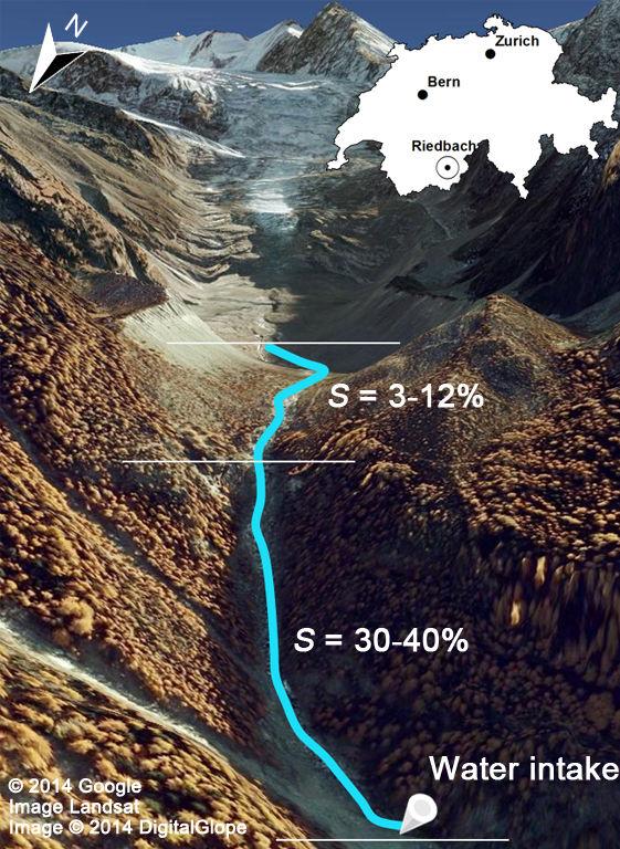
45

46

47 Altidude (m a.s.l.) S=3% S=12% S=40% Fl#01 Fl#02 Longitudinal Profile Fluorometer TLS available Fl#03 Fl#04 Fl#05 Fl#06 Fl# Distance above water intake (m) Fl# Fl#09 Fl#

48