Cres s et Bi omol ecul a r Di s covery Ltd, a l l ri ghts res erved.

Transcription

1 Cres s et Bi omol ecul a r Di s covery Ltd, a l l ri ghts res erved.

2 Table of contents Introduction... 8 What are field points?... 8 Interpretation of field point patterns... 9 About this document Terminology Workflow About FieldTemplater About reference molecules About database molecules Aligning database molecules Similarity scores Proteins as excluded volumes Field and pharmacophore constraints Processing parallelization The main interface Wizard Common concepts and terminology encountered in the Wizard The main window Toolbars Main toolbar Analysis toolbar Style/Surface Chooser Style toolbar Surface toolbar Selection toolbar Protein Display toolbar Measure toolbar D Window Info bar Dock windows Molecules table Tiles / 204

3 Radial Plot and multi-parameter scoring Radial Plot window Radial Plot Properties window Filters window Custom Plot window Forge QSAR Model window Storyboard Project Notes Menus File menu Edit menu Project menu View menu Display menu Run menu Window menu Help menu Right-click menu in the 3D window Right-click menu in the Molecules table Open Molecules dialog CSV Import dialog Protein and PDB import Constraint and Field Point Editor Processing dialog Alignment options Normal alignment Substructure alignment Conformation hunt options Build Model options Field QSAR model options Activity Atlas model options k-nearest Neighbor model options Molecule Editor Molecule Editor quick help / 204

4 Editor right-click menu Rotate mode Select mode Molecular Editor widget and toolbars Saving your changes Activity & Model Manager Column Script Editor Interacting with Blaze Preferences General Appearance Radial Plot Calculations Processing Table Blaze Activity Miner FieldTemplater Conformation Explorer Analyzing conformation populations Style toolbar Filters Histograms Activity Miner Introduction to Activity Miner Running Activity Miner The Activity Miner interface Activity Miner toolbars and 3D Window Disparity Matrix view Top Pairs table Activity view Cluster view Field QSAR models Field QSAR Workflow / 204

5 Building a Field QSAR model Viewing Field QSAR model information Using and Interpreting QSAR Models Using Field QSAR models to predict activity Designing molecules to fit the Field QSAR model Activity Atlas models Activity Atlas Workflow Building an Activity Atlas model Viewing Activity Atlas model information Displaying Activity Atlas models Average of Actives Activity Cliffs Summary Regions Explored Using Activity Atlas models to calculate a novelty score Designing molecules with check of novelty score knn models knn Workflow Building a knn model Viewing knn model information Understanding Forge knn models Using knn models to predict activity FieldTemplater How it works Choosing molecules to use in FieldTemplater Running FieldTemplater The FieldTemplater interface D Window and FieldTemplater toolbars Molecule list Results window Selected Log window Menus The FieldTemplater processing dialog FieldTemplater advanced options Molecules / 204

6 Conformation hunt options Alignment options Templating options Pairwise Constraints Editor Troubleshooting FieldTemplater REST interface to external web services Distributing calculations The science Fields and field overlays Field points Field point generation Field point comparisons The field point overlay technique Notes on fields and molecular mechanics D-QSAR Descriptor generation Scaling Regression Scramble sets Viewing coefficients Viewing variance Activity Cliffs Alignment Similarity and Disparity Matrix calculation Visualisation of activity cliff molecules using field differences Generating templates Generate conformations Generate a list of duos Clique search Consensus alignment Optimize and score the template Appendices Change log and know bugs Molecules table columns / 204

7 Score types available in FieldTemplater File conversion and XED atom types References / 204

8 Introduction Forge is a molecular design and SAR interpretation tool that generates and uses molecular alignments as a way to make meaningful comparisons across chemical series. Given diverse molecules which are active at the same target, Forge will generate detailed 3D models of binding and pharmacophores that help define the requirements of the protein of interest, aiding the synthetic chemist in the design of new actives. When used on a congeneric series the tool can help in library design, give a rationale for the prioritization of compounds for synthesis, give a predictive model of activity using Field QSAR or knn, or help the chemist understand and decipher the SAR of their chemical series using Activity MinerTM or Activity AtlasTM. This manual is mainly aimed at explaining the functionality of the user interface of Forge, and assumes the user is already familiar with the above methods and their terminology. If you want to know more details, the science is discussed in the later chapters of this manual. Forge describes molecules based on their molecular fields, not on their structure. The interaction between a ligand and a protein involves electrostatic fields and surface properties (e.g., hydrogen bonding, hydrophobic surfaces, and so on). Two molecules which both bind to a common active site tend to make similar interactions with the protein and hence, have highly similar field properties. Accordingly, using these properties to describe molecules is a powerful tool for the medicinal chemist as it concentrates on the aspects of the molecules that are important for biological activity. In Forge, molecules can be aligned by using the fields of the molecules, by using shape properties or by using a common substructure. Using the fields gives a protein's view' of how the molecules would line up in the active site, generating ideas on how molecules with different structures could interact with the same protein. Using substructure or common shape properties shows how the fields around a single chemical series varies with activity and in many cases these can be automatically examined to give a 3D quantitative structure active relationship (QSAR) with predictive power for new ideas for synthesis. Forge can also be used to align structurally diverse compounds. This is useful when comparing the SAR of two known active series and looking for comparable substitution sites. With sufficient data, Forge will generate detailed 3D hypotheses for binding through its FieldTemplater' module. Forge serves as a useful tool for compound design. For example, you can use it to design analogues of a known active compound and see how the modifications affect the field pattern, giving insight into how activity can be interpreted in terms of field pattern or new molecules can be scored directly against the a (Q)SAR model for activity. A detailed molecule sketcher and editor underpins the design process with immediate feedback on new ideas. A further application is for library design: small virtual libraries can be compared to a known active molecule to help prioritize scaffold and reagent selection. What are field points? For computational efficiency, Cresset's field technology condenses the molecular fields down to a set of points around the molecule, termed field points'. Field points are the local extrema of the electrostatic, van der Waals and hydrophobic potentials of the molecule. They can be thought of as extended pharmacophores, with the advantages that their position is directly calculated from the molecule's physical properties, and they have size/strength information associated with them (so that, for example, not all H-bond donors are treated the same: some make stronger bonds than 8 / 204

9 others). The generation of field points is described in detail in Cheeseright et al, J. Chem. Inf. Model., 2006, 46, The four field types are used in unison to describe all the potential interactions that a ligand in a specified 3D conformation can make to a protein. Interpretation of field point patterns A representative field point pattern is shown below. Larger field points represent stronger points of potential interaction. Throughout Cresset's software, the field points are colored as follows: Blue: Negative field points (like to interact with positives/h-bond donors on a protein). Red: Positive field points (like to interact with negatives/h-bond acceptors on a protein). Yellow: van der Waals surface field points (describing possible surface/vdw interactions). Gold/Orange: Hydrophobic field points (describe regions with high polarizability/ hydrophobicity). It can be seen that ionic groups give rise to the strongest electrostatic fields. Hydrogen bonding groups also give strong electrostatic fields. Aromatic groups encode both electrostatic and hydrophobic fields. Aliphatic groups such as the iso-propyl group give rise to hydrophobic and surface points but are essentially electrostatically neutral. To generate these fields, we use our XED (extended Electron Distribution) molecular mechanics force field, which uses off-atom sites (which we call XEDs) to more accurately describe the electron distribution in a molecule, as opposed to other force fields where charges are placed at the atomic nuclei only. XEDs are added automatically to any molecule used in Forge. We don't show the XEDs by default, but the option to view them is there if you wish. 9 / 204

10 About this document This document covers the use of Forge and the incorporated Activity Miner and FieldTemplater modules. The modules are addressed in dedicated sections with much of the user interface in common. Common concepts and terms are detailed below. Forge command line binaries are available that reproduce the functionality of the graphical interface. The usage of these binaries is described in individual man' and HTML pages that are installed with Forge. The Forge release notes describe installation instructions, supported platforms and their specifications, last minute changes and that new features in this release. Terminology Some of the specific terminology used in this document is described below Roles All molecules are assigned to a role within the Forge application. Forge is supplied with five default roles that cannot be altered (Reference, Protein, Training Set, Test Set, and Prediction Set). Additional roles can be defined using the appropriate Edit menu entry. Reference molecule Reference molecule' is a molecule that is used in alignment experiments to fit other molecules. The reference molecule(s) describe the information that we know about the protein target and is used as the basis for all alignment experiments. In Forge you can have multiple (up to 9) reference molecules. Template A Template' is a synonym for a set of reference molecules in single fixed conformations and in fixed relative orientation. They can be created by alignment of proteins containing different ligands (e.g. in Cresset's Flare application) or using the FieldTemplater module of Forge. Templates usually contain multiple molecules. Search molecule Search molecule' is a synonym for reference molecule. Search molecules are present in ligand based virtual screening results such as those from Blaze. Protein A Protein' is a region of excluded space around the reference molecule(s) that should not be entered by molecules to align'. Most commonly, the excluded space comes from a protein that has been co-crystallized with the reference molecule or another ligand. A project can have only one Protein'. Training set The 'Training Set' molecules are used in building a (Q)SAR model (Field QSAR, Activity Atlas, or knn) model. Test Set The molecules in the 'Test Set' are used to validate a QSAR model built using the 'Training Set' (either Field QSAR or knn). 10 / 204

11 Prediction Set The 'Prediction Set' is intended to hold all molecules that are not part of either the 'Training Set' or the 'Test Set'. As such they are used to hold result molecules when reading Blaze results files or when fitti ng new molecules to a QSAR or knn model. Molecules to align Any molecule that is not a protein or a reference molecule is described as a Molecule to align', or just as a Molecule' in Forge. For example, these could be molecules that are to be aligned and compared against a reference molecule to understand SAR, they could be newly designed molecules that require 3D validation before synthesis, or they could be molecules retrieved from a virtual screening experiment that are to be visually inspected before choosing which ones to progress. Database molecules Database molecules' is a synonym for Molecules to align'. Focus molecule The term focus molecule' is used in the Activity Miner module to denote the compound at the center of an SAR investigation. It is always drawn first in the 3D window of Activity Miner (on the left or at the top in grid view) and by definition is the row compound in Activity Miner's disparity matrix. Comparison molecule The term comparison molecule' is used in the Activity Miner module to denote the compound that is being compared to the 'focus molecule'. It is always drawn second in the 3D window of Activity Miner (on the right or at the bottom in grid view) and by definition is the column compound in Activity Miner's disparity matrix. 11 / 204

12 Workflow Forge has multiple paths to obtain important insights into existing or designed molecules, depending on the information that is available at the start of the experiment. The Forge wizard will guide you through many of the available workflows and is highly recommended for new users. The workflow is summarized in the diagram below, and key concepts discussed in the following sections. If the 3D shape of the ligands at the target is known then you can provide a single or small set of molecules in a predefined conformation to use as a reference. Forge then aligns a series of database molecules to the reference(s) based on molecular fields, shape, or common substructure. If the conformation of the molecules in the protein is not known but there are multiple, diverse small molecule actives for the target, a pharmacophore hypothesis, such as from the FieldTemplater module of Forge is a good choice for the reference. Failing all else then a generic 3D conformation can be chosen as reference but this brings significant noise into the analysis. About FieldTemplater 12 / 204

13 FieldTemplater searches for common field patterns across the explored conformational space of a set of ligands. A field pattern which can be generated by multiple independent structurally-distinct molecules is likely to be related to how those compounds bind to a common receptor. Field points are used in the early stages of molecular alignment to give an approximate measure of commonality. This is then optimized using the full field. A set of hypotheses is produced, each of which suggests a bioactive conformation for each of the supplied molecules and presents how those bioactive conformations relate to each other. Each such hypothesis is termed a template' which can be used as a reference in the main Forge application. For details on how the FieldTemplater module operates, please see the FieldTemplater section. About reference molecules Suitable reference molecules are highly active molecules, preferably in the bioactive (protein bound) conformation for the protein of interest. This bioactive conformation could come from a proteinligand x-ray crystal structure or from a dock of the ligand into the protein. In the absence of protein structure data, the information could come from the FieldTemplater module of Forge or from a pharmacophore model. Lastly, a reasonable guess of the conformation can work well in cases where the structural diversity of the ligands is low. If you choose to use a 2D molecule, Forge will convert it into a 3D conformation before proceeding. Multiple reference molecules Alignments to a single reference molecule generally work well. However, if you have two known actives that each occupy a slightly different part of an active site then it might be better to use both molecules, pre-aligned, as a single reference for the alignments. Alternatively, if a large number of diverse ligands are known, then a multi-molecule reference will probably describe the diversity of chemical features that are present better than a single molecule reference. Note that the calculation time for the alignments can depend non-linearly on the number of reference molecules used: using three reference molecules will take six times as long as using just one. Multi-reference-molecules are used by the software to find alignments of the database molecule that match each reference well while keeping the alignment of the reference molecules to each other fixed. In practice, this involves optimizing the alignment against each molecule within the reference simultaneously with the score being the average or maximum of the individual alignment scores. Because the alignments of the reference molecules do not change, they must be pre-aligned before the experiment starts. If this is not the case, then Forge will not produce meaningful results. Note that although a maximum of 9 molecules can be used in the reference role, Cresset recommend a maximum of 6 to enable the experiments to complete in a reasonable time. About database molecules Molecules that are not reference molecules are termed database molecules'. They can be loaded into Forge from a file, drawn directly using the Molecule Editor, or pasted from a chemical drawing package like ChemDraw. Using pre-calculated conformations Database molecules can be added as conformation populations, thereby bypassing the conformation hunt within Forge. To save computing time, Forge filters out conformational enantiomers for achiral molecules during the conformation hunting process. The field alignment process is then performed against each stored conformation and its mirror image. As a result, the effective number of 13 / 204

14 conformations examined is double the number stated for achiral molecules. If you choose to import conformations from another program, conformational enantiomers will still be calculated for achiral molecules at alignment time unless you deselect the Invert achiral imported confs' option in the alignment options of the processing dialog. Protonation states Protonation states are controlled by an option in the file import dialog box. The default setti ng is for Forge to use the protonation state that is represented (drawn) in the file. You can alternatively tell Forge to re-assign the protonation state of all molecules on input. Forge's built-in rules can only approximate a pka (e.g., diethylamine and morpholine are treated identically) and simply assigns protonated or deprotonated states assuming a ph of 7. Therefore, for molecules with a pka around 7, only one state is included and this might be incorrect. In this situation, SAR of close analogues can often guide the protonation state. Alternatively, the molecule could be input twice, once in the protonated state and once in the deprotonated state, and both will be fitted to the template. If the molecule is loaded in the wrong protonation state, it can be corrected using the Molecule Editor. Simply right click on the molecule and choose Edit molecule'. Use the +' or -' button in the Elements widget and click on the charged atom. Within Forge, all charged groups are given extra ( formal') charge. However, using a full charge (+1 for positives, -1 for negatives) results in a field pattern that lacks subtlety and is dominated by that charge. To correct this, a charge scale factor is applied to all charged groups. This can be thought of as a solvent' shell (or a local dielectric) around the charged group. By default, Forge applies a charge scaler of 0.125, i.e., an ammonium would have a formal charge of and a carboxylate a total formal charge of spread across both oxygens. Aligning database molecules Forge aligns molecules using fixed conformations. Molecule conformations can be read into Forge or can be calculated by the program. In either case, the conformations are aligned to the reference molecule in two stages. In the first stage, the field points around a molecule are used to generate an initial alignment. In the second stage, the initial alignment is optimized to get the best possible score. In this second stage, it is possible for Forge to use an excluded volume' file that defines a region of space around the reference molecule that acts as a constraint on the alignments. Typically excluded volume files are derived from protein-crystal structure data. An outline of the fitti ng process is shown below. Molecules can also be aligned using an alternative substructure based approach. Where the use of field points to generate alignments is akin to a protein centric view of the alignment, a substructure alignment is a ligand centric view. The advantage of this approach is that the differences between molecules that lie in the same series are easier to interpret, particularly when using ligand-centric computational techniques such activity cliff analysis (Activity Miner, Activity Atlas) or building quantitative activity models (FieldQSAR, knn). 14 / 204

15 Similarity scores The score is an important factor in deciding the validity and potential activity of alignments and molecules. However, it is not the only factor to be considered before embarking on the synthesis of a compound designed in Forge. The top-scoring result is the one that is the most similar to the target molecule in terms of fields and shape. That doesn't necessarily mean that it is the most likely to be active, and certainly doesn't mean that it's the one you want to make first. The absolute value of the scores isn't that informative in isolation, largely because the scores provided are the similarity of the result molecule to the target molecule. If you are replacing only a small part of a large molecule, then the large number of atoms in common between the reference and the results will mean that the similarity values may all fall in a range of In other words, the scores are useful for ranking the results (higher-scoring result molecules are more similar to the reference than lower-scoring ones), but don't pay too much attention to the absolute numbers and don't compare the numbers between different reference molecules. Sometimes it may seem that the field points of two molecules in a particular alignment don't match up. This is because the scoring algorithm uses field points as sampling points of the true field around a molecule. To score two molecules the field of B is sampled at the locations of the field points of A and vice versa. Thus, the field points for the result and the target molecules may not be exactly 15 / 204

16 coincident, but if the true fields show similar properties at the field point locations, the field similarity and hence, the score will be high. Viewing the field surfaces for the target and result molecules can be instructive. Please consult Fields and fields overlay for more information. It is possible to get strange scores from Forge. This usually occurs when some large field constraints have been applied. If field constraints are violated, then a penalty is applied both to the raw field score and the raw shape match score. When normalized, this can then lead to very low or even negative field and shape similarities. Proteins as excluded volumes Where a protein structure is available it is used in Forge as an excluded volume, i.e. to down-weight alignments that enter certain regions of space. Alignments that make the database molecule clash with the excluded volume molecule are penalized, with the penalty getti ng higher the more atoms that clash. Ligands that are aligned in Forge are shown within the protein where potential interactions can be analyzed. Although an excluded volume is usually derived from a protein crystal structure this is not a restraint. Any molecule can be used as an excluded volume. The only information that is used from the excluded volume molecule is the position of the heavy atoms, so you need not worry about protonation states, tautomers and the like. The excluded volume is deliberately made quite soft'. As a rough guide, sticking a single atom from the database molecule into the protein will give a penalty of ~0.02 to the similarity score. In other words, pushing a methyl or ethyl group into the protein generally only has a small effect on the score, but placing an entire phenyl group into it is significantly disfavored. Field and pharmacophore constraints Constraints bias the alignment algorithm to down-score results that do not satisfy the constraint. In Forge there are two separate types of constraints - field constraints and pharmacophore constraints. 16 / 204

17 Field constraints offer the opportunity to specify a particular type of field must be present in the aligned molecule. This could be a hydrophobic point which forces the alignments to fill a particular pocket or an electrostatic point to enforce an interaction. Pharmacophore constraints force aligned molecules to have a particular feature - H-bond acceptor for example - at a specific position. It is appropriate to use a field constraint when you are certain that a particular field point is critical to activity or when you wish to force Forge to give you a specific alignment that might otherwise have been missed. For example, you might choose to constrain the field points associated with the an edge-to-face aromatic interaction or where you want an interaction but it can be matched by H-bond donors and other electropositive features such as the aromatic hydrogens in the example above. It is appropriate to use a pharmacophore constraint when you are certain that a particular interaction requires transfer of electrons (as in H-bonding or metal binding) in addition to the electrostatic character of the interaction. When a field constraints is applied to a particular feature the user is applying a penalty to any alignment where this field point does not sample a field that is the size of the constraint applied. Cresset's method of alignment uses the field points of one molecule (e.g. A) to sample the true field value of the second molecule (e.g., B) in a given alignment. If the value of the field that is sampled by a constrained field point is lower than the constraint value specified by the user, a penalty is applied. The size of the penalty is dependent on the size of the field point that is being constrained, the size of the field being sampled, and the size of the constraint. The relationship between these factors is non-linear with small differences being penalized proportionally less and large differences being penalized significantly more. If a molecule can fulfill the constraint without the alignment changing, no penalty will be applied and hence, the score that is obtained with a field constraint present will be identical to that obtained when it was absent. In practice, most molecules that are aligned using field constraints will have different scores to those obtained without constraints. Pharmacophore constraints are, in effect, a tighter constraint on the alignment than a field constraint. Where field constraints allow matches across chemical features, pharmacophore constraints are limited to matching specific functional groups (for example, the donor-acceptor-donor pharmacophore motif in kinase hinge binders). Alignment that do not place a suitable atom on top or close to the constrained atom cause a penalty to be applied to the score. However, pharmacophore constraints go beyond traditional H-bond donor/acceptor definitions to include, for example, covalent centers and metal binding motifs giving the ability to ensure that key warheads always align in the correct positions. Please refer to Constraint and Field Point Editor for details on defining field and pharmacophore constraints. Processing parallelization Forge runs on multiple processors or cores on your local machine. It can also (with the appropriate license) run on remote machines. There are multiple options to achieve this but the easiest is to use a small server program (CEBroker) that will receive calculation requests from client machines and submit calculation jobs ( FieldEngines') to a Linux cluster. For more information please contact Cresset support. 17 / 204

18 The main interface When you start Forge, you are offered the choice of starting a new experiment or opening an existing experiment. You can exit to the main application interface by closing the pop up box or hitti ng the Esc key. Clicking New project' opens the Wizard (described below). This is the simplest way to start using Forge, and will guide you through the various types of experiment that you can perform with Forge. Wizard To enter the wizard, click on New project' on startup or click the new project icon ( ) on the Main toolbar. When the wizard starts you are given a choice of experiment to setup (shown and detailed below). Blank Project Exit the wizard and return to the main application with a blank project. You will be prompted to save any open projects. Open Project Open an existing project in place of the current one. After selecting the project to open, you will be prompted to save the existing project if changes have been made since it was last saved. View Molecules in 3D Open molecules to view them in Forge. This can be used to view the results of a Blaze virtual screening experiment, or simply to look through a set of molecules in 2D or 3D. When you select this option, the file browser window will open to select the molecules to view. Once files have been selected, their filenames are displayed in the window. Multiple files from multiple locations (including the clipboard) can be specified. Clicking Finish' loads the molecules from the specified files. Note that Forge will automatically detect protein excluded volumes and reference (query) 18 / 204

19 molecules in any Blaze results files that are in SDF' or bmf' format if the molecule read mode is set to Autodetect' in Open Molecule dialog. Align Molecules This experiment will align molecules to a reference molecule to enable visual inspection of how the molecules and their field patterns differ. The experiment is an excellent way to understand how different chemotypes relate to each other in 3D, or to understand the causes of activity when you do not have enough data to build a full field activity model. Choose this experiment if: you have a reference or template to be used for aligning molecules you do not have detailed activity data for the compounds that you are studying the compounds have only a small difference in activity (< 3 log units) the compounds come from multiple chemotypes you want to visually inspect alignments before progressing to build a Field QSAR model or look for activity cliffs using the Activity Miner module. Once you have chosen this experiment, the subsequent steps of the wizard will guide you through the setup process. View Molecules in Activity Miner This option is used to examine molecules in the Activity Miner module. The first stage is to choose whether molecules will be loaded pre-aligned or requiring alignment. The steps are initially identical to those for building a Field QSAR model except that the Activity Miner interface will launch once a project has alignments and activity values for all molecules. Activity Miner is an excellent way to explore and interpret SAR. Build an Activity Model This experiment is similar to the align molecules experiment, except the final alignments are used to prepare a model of binding that describes the known SAR or predict the activity of closely related compounds. There are three types of model in Forge - a Field QSAR model' that is derived from field 19 / 204

20 sample values across the training set and predicts activity; an Activity Atlas model' that summarizes activity data in a 3D map of critical, allowed, and explored regions of shape, hydrophobics and electrostatics; and a k-nearest Neighbor' model of activity. All of the models can be applied to the design of new molecules in a visual (Field QSAR, Activity Atlas) or quantitative (Field QSAR, knn) manner. Choose this experiment if: you have a reference or template in 3D which can be used to align molecules or you have molecules in a predetermined alignment you have detailed activity data for the compounds that you are studying the compounds cover at least 1.5 log units of binding activity the compounds are largely part of a single chemotype Once you have chosen this experiment, the wizard will guide you through the experimental setup. Fit Molecules to an Activity Model Use this option if you or a colleague has generated an activity model already and you wish to use this to design or score more compounds. Choose this if: you have an activity model already you want to design or score compounds against the model The subsequent steps of the wizard will ask you to load the model and reference molecule from an existing Forge project and load molecules to be aligned to the reference molecule. If your molecules are already aligned then when the processing dialog appears you can close the window without starting an experiment. All aligned loaded molecules will have predicted activities automatically calculated (where these are appropriate) and displayed in the Pred' column that is associated with the model. Create a Pharmacophore with FieldTemplater FieldTemplater is used to create a 3D description of how molecules bind to the target of interest. It cross-compares active molecules to produce hypotheses that represent the bioactive conformations of the input molecules. This is the place to start if: you do not know exactly how your ligands interact with the protein you have 3 or more diverse molecules, believed to bind at the same protein site with reasonably good binding constants If you choose this option then you will be asked to give the FieldTemplater project a name and to load the molecules that are to be used before the FieldTemplater module is opened. 20 / 204

21 Common concepts and terminology encountered in the Wizard Reference Molecule (Template) The reference molecule is used to align other molecules within Forge. It is usually one or more 3D conformations of molecules in a predetermined orientation. If possible the reference molecule should be in the bioactive conformation - i.e., the conformation that is present when the ligand is bound to the protein of interest. However, you can upload a molecule drawn in 2D and Forge will convert it to a 3D conformation to be used as a template for the alignment of all other molecules. You can paste your reference molecule directly into the wizard using the Paste' button or extract a ligand from a protein-ligand crystal structure using the Protein' button. In choosing the reference molecule, we recommend that if possible you choose a highly active molecule. You can use multiple molecules as a reference but these must be pre-aligned so that they exist on the same coordinate space with equivalent groups overlaid. If you are using multiple molecules as a single reference then they must exist as separate entries in one file or as separate files. If you would like to further discuss the choice of molecule to use then please contact Cresset support. Database molecules A database molecule is any molecule that is not a reference molecule or template molecule. They can have known or unknown activity, be part of a test or training set or compounds for which a prediction of activity is required (part of the prediction set). They can be loaded in SMILES format, as SMILES in a csv file, or as 2D or 3D conformations in an SDF, mol2 or xed file. You can specify as many files as you like, but the total number of molecules is limited by how much memory your system can give to Forge. If you wish to consistently work with large datasets then please talk to Cresset support about the command line version of Forge. Each file in turn is read, validated, and converted internally into xed format. During this process a Converted <n> molecules' progress dialog box appears. If fewer molecules appear in the list than there were in the file then there may have been a problem with the molecule conversion. Check that any molecule which failed to read properly is correctly saved in the format that you specified. Protein molecule This is optional. You have the option to import a molecule (usually a protein) that specifies regions of space that will be marked as an excluded volume'. That is, any alignment that places one or more atoms inside this volume will be penalized. The penalty is proportional to the number of atoms entering the volume. By design, the volume specified is soft'; small infringements into the region do not significantly affect the alignment score. The pharmacophoric properties of protein molecules are not used; they are treated purely as steric volumes. Typically, an excluded volume comes from the protein atoms in a protein-ligand x-ray structure. You will need the protein atoms in mol2, pdb or SDF format. Only the atoms within 10 Å of the ligand will be used in the calculation and there is a limit of around 2500 residues (25,000 atoms) on the size of the excluded volume. Generally we recommend removing waters and mobile loops from the protein as these are not used in the alignment directly. If you have loaded a reference molecule using the Protein' button then the rest of the protein will be loaded automatically. Field and pharmacophore constraints This condition is optional. In summary, including a constraint introduces a penalty score to any alignment that does not match the field or pharmacophore constraints. Use this feature to mark field points or pharmacophoric features that are clearly important for activity. The more constraints the 21 / 204

22 better the alignments will be for congeneric series but at the expense of applying some personal bias. Constraints are implemented using the Constraint and Field Point Editor window. We recommend that constraints are used sparingly. The Processing Dialog This is the final step of setti ng up any experiment. You are asked to specify how each stage of the calculation is performed. A full description of all the available options appears in the Processing dialog section. The Conformation Hunt' control has a major effect on the speed and accuracy of the alignments that are generated. The four options ( Quick', Normal', Accurate but slow', Very Accurate and Slow') affect the number of conformations that are kept for the alignment step and the degree to which each of these is minimized. Cresset's advice is to use the Accurate' setti ng wherever time allows as this will usually give better results than the Quick' or Normal' setti ngs. However, if you have a set of database molecules that are uniformly small then you may find it more convenient to use one of the faster setti ngs. Important: If you do choose to keep a large number of conformations for a large number of molecules (>100) then you should consider reducing the memory footprint of the application by going to the Forge Calculations preferences and checking the box marked Delete unused conformations'. Alternatively the excess conformations can be removed at any time using the Delete unused conformations' option in the Edit menu. The Alignment' setti ngs allow you to align quickly ( Quick') or using the default setti ngs ( Normal'). In either case, the database molecules will be aligned to all of the references using a 50/50 mix of shape and field similarity. The third setti ng ( Substructure') is different: it modifies how the conformation hunt is performed by matching the database molecule to the most similar reference molecule based on their maximum common substructure (MCS). This forces the alignment to match the common substructures closely, with field/shape scoring controlling the conformation of the parts of the molecule not contained in the MCS. The Build model' setti ngs control the type of model the application should build. There are five different calculation types plus a No calculation' option. The Field QSAR' models create a Field QSAR model with variants to choose whether a full set of y-scramble experiments should be done or skipped and whether the alignment score should be used to weight the contributions of different molecules. The Activity Atlas' option creates a model that summarizes the regions of space that have been explored or have are associated with activity changes. A k-nearest Neighbor' model can be used to predict the activity of molecules that are closely related to the training set. The Model Activity' is used during model building. If a suitable column is not automatically detected then the Activity & Model Manager (Project menu Manage Activity & Model Data) can be used to manually select the column in the results table that contains the activity values for your compounds. 22 / 204

23 Detailed control of the behavior of these three stages is available by pressing the 'Show Options' button, or the Setti ngs icon near each calculation method. This gives access to the advanced options that give detailed control of each stage of the experiment. Information, warnings and potential errors in the calculation configuration are displayed at the bottom of the processing window. Hovering the mouse over the warning gives a more detailed message. Where there are multiple messages these can be scrolled using the displayed arrows. The 'Start' button on the processing dialog starts the experiment and opens (or returns to) the main graphical user interface. The main window Toolbars There are eight toolbars in the main Forge GUI. They can be viewed or hidden using the Windows Toolbars menu and repositioned using the handle on the left or top of the toolbar, or by choosing Reset Layout' in the Windows Toolbars menu. The Main toolbar is used to start new projects with the Wizard, open existing projects, reference or database molecules, to start calculations and add/edit fields and field constraints. The Analysis toolbar gives access to the Conformation Explorer for viewing and analyzing the conformations saved for each selected molecule, Activity Miner for rapid assessment of the structure-activity and selectivity relationships around a set of molecules, and Custom Plots of data from the results table. The Measure toolbar is used to measure distances, angles or torsions in the 3D window. The remaining toolbars are used to change the display in the 3D window. The Style-Surface Chooser controls which molecules are affected by the Style Toolbar and Surface Toolbar. The Selection Toolbar 23 / 204

24 controls the visibility of molecules. The Protein Display toolbar controls how protein molecules are displayed. Main toolbar In addition to standard file functions (new project, open file, save project) the main toolbar controls the start of calculations within Forge and enables the addition and editing of fields and field constraints. Analysis toolbar The Analysis toolbar contains functionality for viewing and analyzing the conformations saved for each selected molecule with the Conformation Explorer, assessing the structure-activity and selectivity relationships around a set of molecules with Activity Miner, and creating custom plots of data from the results table. 24 / 204

25 Style/Surface Chooser The Style-Surface Chooser sets the domain of applicability or relevance of the display and surface toolbars. Possible values for the toolbar are: All Ligands All References Protein Model All Molecules Selected Molecules Picked Molecules For example, setti ng the Style-Surface Chooser to Selected Molecules' and clicking the change molecule color button on the Style Toolbar causes the new color to be applied to just the selected molecules. No other molecules are changed. Equally, setti ng the Style-surface chooser to Protein' and clicking the add molecular surface button on the Surface Toolbar causes surfaces to be calculated for just the molecules that have been loaded as excluded volumes. Style toolbar The Style toolbar controls the style applied to molecules in the 3D window. All its functions can be accessed through the Display' menu. Note that the application of each button is controlled through the Style-Surface Chooser on the display toolbar. Thus clicking the Reset Display' button ( ) whilst the chooser is set at Selected molecule' resets the display of just molecule that is currently selected and not of any other molecules. 25 / 204

26 Surface toolbar The Surface toolbar is used to show, hide and remove molecular and field surfaces to any molecule. Like the Style Toolbar, changes are only applied to the molecules specified by the Style-Surface Chooser. Field surfaces (positive, negative, shape, and hydrophobic) are shown at the contour level given in the spin box. When only two molecules are selected, the field surface can be switched into Difference' mode. In this mode the chosen field surfaces are displayed as a difference between the two molecules in the 3D display. Regions that have the higher value (by the amount shown in the spin box) are drawn on each molecule. 26 / 204

27 For example, the positive field surface difference (top) and absolute positive field surface (bottom) are shown for trifluoroacetic (left) and acetic acid (right). The acid proton is absolutely positive in both cases (bottom) but the trifluoroacetic acid is more positive and hence has a surface present in difference mode. Similarly, comparing the CH3 group of acetic acid to the CF3 of trifluoroacetic shows that the CH3 is both positive in an absolute sense and more positive than the CF3 group in the difference view. Selection toolbar The Selection toolbar controls what is shown in the 3D window. It also controls whether the 3D window operates in the native overlaid' mode, where every molecule is shown simultaneously overlaid with the other molecules, and grid' mode where each molecule is displayed in its own grid square. The View Model 3D Plots button opens a sub menu that controls the display of features of the current QSAR model. The controls reproduce those on the 3D view tab of the QSAR Model window and change depending on the type of model that is active (set with the View View Model menu entry). 27 / 204

28 Protein Display toolbar The Protein Display toolbar is used to control how the protein is displayed in the 3D window. The ASite' button cuts down the atomic display of the protein to just the active site (the residues within a radius of the reference molecules, specified in the preferences or by using the active site radius spin box). The Ribb' button enables display of the protein backbone as a ribbon: a drop-down menu enables the selection of different ribbon styles. The HBnds' button displays potential hydrogen bonds between the selected molecule and the protein excluded volume (using green lines) together with regions where the current molecule clashes with the protein (orange lines). Note that the hydrogen bond markers are drawn depending purely on the geometry: no computations of actual hydrogen-bonding strength are made. Measure toolbar The measure toolbar is used to investigate distances, angles and torsions together with intermolecular hydrogen bonding within the 3D window. To make a measurement, hold down the Shift key, click the atoms in the 3D window that will be used and then click the Measurement button. Selecting two atoms causes a distance to be calculated, three atoms gives an angle, four atoms gives a torsion. The Clear Measurements button clears the measurements between the selected atoms. If no atoms 28 / 204

29 are selected, then clicking on the Clear Measurements button will clear all the measurements in the 3D window. 3D Window The display in the 3D window is controlled by all the other features of Forge. Cresset believes that visual inspection of the 3D alignment is the best way to choose both successful alignments and good molecule correspondences. The 3D window can be expanded to a fullscreen view using the F11 key or from the right-click menu in the window. To return to the normal view, press F11 again or the Escape key. While in fullscreen mode, all the mouse and keyboard shortcuts function normally, enabling navigation of results in fullscreen mode. The current state of the 3D window can be captured to the Storyboard window for later recall. Scenes can be captured using the camera button on the Storyboard window, by selecting the appropriate entry when right- clicking on a molecule in the 3D window or by pressing the F4 key. The main control for the 3D window is the mouse. The available functions (with the mouse focus in the 3D window) are: Mouse controls Control Effect Left mouse button Rotate view around x/y axes Right mouse button Translate view Mouse wheel up/down Zoom in/out Wheel mouse button press and drag Zoom in/out ALT + Left mouse button Zoom in/out Ctrl + Left mouse button Rotate view around z axis <' and >' or,' and.' or [ and ]' Zoom in/out Shift + Left mouse button drag Clip in the front Z-plane (up or down). The current clip value is shown in the lower right corner of the 3D window. Shift + Right mouse button drag Clip in the back Z-plane (up or down). The current clip value is shown in the lower right corner of the 3D window. Left mouse click on an atom Select atom under mouse Note that many of the display toggles have keyboard shortcuts (e.g., f' to show/hide field points). The keyboard shortcuts are shown in the menu entries for the various display functions. Selected keyboard shortcuts are shown below. Detailed visual guides to the keyboard shortcuts for key parts of the application can be requested to Cresset support. Keyboard shortcuts Domain Shortcut 29 / 204 Action

30 Controlling the Style-Surface Chooser Controlling the Molecule and Field Display Style Showing labels Changing What is Displayed Interacting with Molecules table Ctrl-A All Ligands Ctrl-R All References Ctrl-M Selected Molecules Ctrl-P Protein C Capped Stick Atoms T Thin Stick Atoms H Show Hydrogens F Show Fields + Display Positive Electrostatic Potential - Display Negative Electrostatic Potential Ctrl-Shift-R Reset Display Shift-I Display Atom Index Shift-E Display Atom Elements Shift-Y Display Atom Type Shift-C Display Atom Charges Ctrl-Shift-C Display Atom Formal Charges Shift-H Display Chirality Shift-F Display Fields Size Shift-X Reset Labels P Show Protein A Toggle Protein Active Site Only R Toggle Protein Ribbon Shift-1 Show Flat Ribbon Shift-2 Show Tube Ribbon Shift-3 Show Cartoon Ribbon (default) Ctrl-G Change 3D Display into a Grid Ctrl-(0-9) View Activity Atlas Surfaces Ctrl-(1-2) View Field QSAR Coefficients Ctrl-F View Field Contributions to Predicted Activity (Field QSAR models only) V Show Field QSAR Model Variance while pressed (if turned on with Ctrl-1 or Ctrl-2) Space on a Mark Current Molecule as 30 / 204

31 molecule Favorite Open Tree Next/Previous Visible Item in Table Go to Parent or Close Tree Ctrl-Space Clear all Favorites Field Colors Forge can display a number of different field types both as surfaces and points. Most colors can be customized using the Appearance preferences. A quick explanation is given below using the default colors. If you are unsure as to what a given field point represents, then you can hover the mouse over it for an explanatory tooltip. Field kind Name Meaning Molecular field. The shape of these field points can be changed in the Display menu or with the Style toolbar. Negative Negative electrostatic potential Positive Positive electrostatic potential Hydrophobic Hydrophobicity (grease) vdw Shape/van der Waals descriptors Positive More positive/less negative electrostatic potential leads to higher activity Negative More negative/less positive electrostatic potential leads to higher activity Sterics+ More steric bulk leads to higher activity Sterics- More steric bulk leads to lower activity (excluded region) Electrostatics+ The molecule's electrostatic field is increasing predicted activity here Electrostatics- The molecule's electrostatic field is decreasing predicted activity here Sterics+ The molecule's steric potential is increasing predicted activity here (i.e. the steric bulk here is good) Sterics- The molecule's steric potential is decreasing predicted activity here (i.e. the steric bulk here is bad) Electrostatic variance Larger points mean more difference in the electrostatic potential here across the training set Steric variance Larger points mean more difference in the steric potential across the training set Activity Atlas (surface) & Field QSAR (points) model colors. Press Ctrl and a number 19,0 to toggle the model components. Field QSAR: Field contribution to predicted activity. Press Ctrl-F to toggle on/off. Field QSAR Model variance. Press Ctrl-Shift-1 or CtrlShift-2 to toggle, or press and hold v' while model coefficients are shown. 31 / 204

32 Info bar The info bar is directly below the 3D window. It is used to present information about the current molecule(s) and to facilitate rapid navigation and assessment of all the 3D alignments. It contains buttons for navigation through the alignments [ ] (equivalent to pressing up and down keys), a button for marking the current alignment as a favorite' [ ] (equivalent to pressing the space bar) and the score, activity, predicted activity/novelty (according to the selected (Q)SAR model), and title of the current molecule together with the number of molecules that are selected and the number of favorites that have been set. Dock windows In addition to the main 3D window, the main Forge application contains a number of Dock' windows that can be enabled or disabled, moved within the main window or to a separate monitor, or closed completely. Some of these, such as the QSAR model information window, are only shown when needed (e.g., when viewing 3D QSAR, Activity Atlas or knn models). Any dock window can be shown using the appropriate entry in the Window Docks menu. Molecules are displayed in two separate dock windows. The Molecules table' displays structures together with all the data that has been calculated or loaded into Forge. The Tiles' view shows selected data only, but enables the display of more molecules. Each of these is described in detail in the Molecules table and Tiles sections. Molecules table The Molecules table shows all the molecules that have been loaded into Forge. The molecules are organized into categories or Roles'. There are five default roles in the table: Reference molecules, Protein (excluded volumes), and database molecules which are categorized as Training Set, Test Set, or Prediction Set. Additional roles can be created using the Molecule Role Editor (Project menu Create/Delete Roles) or using the right click menu on the table. Within a role, each molecule is shown in the table as a separate row. Molecules can be dragged and dropped into other roles, or moved with the right-click menu. Note that 'Training Set' and 'Test Set' roles have special uses for developing QSAR and Activity Atlas models but function like any other role in all other circumstances. If the molecules were read from SDF files then any extra data that was available in the SDF file will be presented as a new column in the table. A number of physical properties are calculated for all molecules that are loaded into Forge. The Table preferences (Edit menu Preferences) controls which columns are displayed or hidden by default for new Forge projects. Note that Forge will attempt to automatically recognize columns containing activity data and use these to calculate properties such as ligand efficiency (LE) and lipophilic ligand efficiency (LipE or LLE). The Activity & Model Manager window (Project menu Manage Activity & Model Data) gives full control over the handling of activity columns. Columns can be colored according to how the value fits a profile (e.g., TPSA green, <20 or >100 red). The profile is set up in the Radial Plot Properties window. The colors used are set up in the Table preferences, and applied according to the Radial Plot Properties. 32 / 204

33 Once a database molecule has alignments (calculated or read in), the score of the top scoring alignment or of the preferred alignment will be displayed in the molecule's main row (Sim column). Clicking on this row shows this alignment in the 3D window. Additional alignments are accessible for any molecule by clicking on the expand row' button on the left hand side of each row. Additional alignments are clustered into a hierarchy with truly different alignment presented above alignments that are only minor variations of a higher scoring result. Reference molecules are shown with a different background color to database molecules. All molecules in the Molecules table can be edited by double-clicking the 2D structure, or by highlighting the molecule and selecting the appropriate entry under either the right-click or Edit menus. Tiles The Tile view shows a compacted version of the Molecules table. Each molecule within a role is displayed on a Tile'; tiles are laid out in the window horizontally then vertically, and can be shown as either Large', Medium' or Small' (right-click menu Tile Size). The data that is shown on a tile is configurable choosing 'Project Show/Hide Tile Items' or by right-clicking on a tile and selecting Choose Tile Data'. Each tile can hold both pictorial data (such as the structure or radial plot) and numerical or string data. Structures, radial plots, notes and tags use the full height of the tile and hence occupy a single column within the tile. All other data is presented as a single row with the number of rows on each tile depending on the size of the tile (Large tiles have 10 rows, Medium have 7 rows, Small have 5 rows). The molecules in the Tile view are divided into Roles' in exactly the same way as in the Molecules 33 / 204

34 table. Within each role the tiles can be sorted by any of the columns in the main Molecules table (right-click menu Order Tiles by). Radial Plot and multi-parameter scoring To aid in the optimization of multiple parameters the radial plot is used to summarize and condense numerical data from multiple columns into a single picture and number that can be used for sorting or filtering. The radial plot for each molecule is displayed in the Molecules table, optionally in the Tiles view and in the Radial Plot window for the selected compound(s). The data that is initially used in the radial plot and the way it is combined into a single number is set using the Radial Plot section of the preferences. However, data can be added, removed, reordered, or rescaled in the specific project using the Radial Plot Parameters Window. The radial plot is based on the idea that molecule properties that are 'perfect' should be displayed at the center of the radial plot. Thus, a molecule with perfect or near-perfect properties should have a radial plot with a small encapsulated area (shown in green). Conversely, poor properties would be plotted at the edge of the radial plot such that a molecule with sub-ideal properties would have a radial plot with a large enclosed area. This can be reversed using the Radial Plot preferences. The plot properties are combined into single score that represents the fit of this compound to the overall project properties. The score is created as follows: 1. Normalize the property fit to the radial plot parameter function to an individual value between 0 and 1 where values at the edge of the plot receive zero and those at the center 1 34 / 204

35 2. Multiply the individual values by a weighting for this property 3. Sum all individual values 4. Normalize the sum to give a combined score with a value between zero and 1. In combining plot properties, the weight that is applied to the individual property is used to set its importance to the overall project profile. For example, if the project is prepared to accept lower activity in return for a better TPSA profile, then the weight of the Activity property could be reduced below 1 or the weight of the TPSA property could be set above 1. The score is displayed above the radial plot whenever it is displayed. Sorting the Molecules table or the Tiles using the Radial Plot uses this score. The score is also used to adjust the background color of the radial plot according to color scheme defined in the Table preferences (the default is red for molecules with a poor profile and green for molecules with a good profile). While the color of the radial plot window describes the overall fit to the project goals, the individual shape of the plot indicates which how this score is composed and where the molecule is sub-optimal. The radial plot profile for each numerical column can be defined in the Radial Plot preferences, even if the column is not selected for display in the Radial Plot. The radial plot profiles can also be used to color the column data in the Molecules table: the color scale can be customized in the Table preferences (the default is red for poor values and green for good values), and the option to 'Color Table by Radial Plot' can be chosen so that every column that has a profile set in the preferences is colored in the table. Radial Plot window The Radial Plot window summarizes the data for the selected compounds. It is useful when setti ng up the plot and when examining data values for multiple molecules. Where a single compound is selected the Radial Plot window duplicates the data that is present in the Molecules table but on a larger scale. Hovering the mouse over any data point will display the title of the molecule and the value for that parameter. Selecting multiple molecules/alignments causes multiple radial plots to be displayed in line mode with a different color used for each molecule. Again, hovering the mouse over any data point gives information about that point in a tooltip. Clicking on any line in the plot causes the molecule that 35 / 204

36 gives rise to that line to be scrolled to the top of the Molecules table. Double clicking a line in the plot switches the selection to be just the molecule that corresponds to that line. Radial Plot Properties window The Radial Plot Properties window is used to set up the display of the radial plot and the weighting that is to be used in combining properties into a single score. Where there is no activity data, 4 properties are displayed by default (Sim, MW, SlogP, TPSA) with equal weighting. However, the Activity and Ligand Efficiency properties are automatically added if activity data is present. All properties are used with a predefined set of ranges and weights, however, the default properties for ranges and weighting can be set using the Radial Plot preferences. To add properties to the radial plot, simply select the appropriate column from the drop down list at the top of the window. The order of properties in the radial plot is set by the order of the properties in the radial Plot Properties window (clockwise from top to bottom). The properties can be reordered by clicking and dragging the handle to the left of the property name (see picture above). Clicking the button removes the property from the radial plot. Clicking the button displays or hides a distribution diagram showing the range of values for the property in this project together with the average and standard deviation for this value and how the function maps these values in the radial plot. Changing the parameter values in the spin boxes or dragging any of the dashed vertical lines changes the way the chosen function is applied to the property values. The left side (Y-axis) of the distribution diagram is a zero to one scale representing the output of the function where C represents the center of the radial plot and E represents the edge of the radial plot. The values from the property can be plotted using four different functions to represent good and poor values (selected from the drop-down menu), each of which is controlled by the parameters 36 / 204

37 presented in the spin boxes. Cutoff A simple linear scale where values below the 'Lower Cutoff' appear at the edge of the radial plot and values above 'Upper Cutoff' appear in the center of the radial plot. Use for properties where bigger numbers are better (such as Activity on a log scale) Cutoff Inverted As above except the function is inverted. Values below the 'Lower Cutoff' appear at the center of the plot, values above the 'Upper Cutoff' appear at the edge of the plot. Use for properties where smaller numbers are better (such as MW or Rotatable Bond Count). Range Values within the 'Perfect Range' are considered perfect and plotted at the center of the radial plot. Values that lie outside the 'Acceptable Range' are plotted at the edge of the radial plot. Use for properties that have an acceptable range of values (such as TPSA). Range Inverted Values within the 'Bad Range' are assigned as poor and plotted at the edge of the radial plot, values outside the 'Acceptable Range' are shown in the center of the plot. Filters window The Filters window enables you to select only the molecules that conform to a set of rules or filterse.g., SlogP must be < 5, MW must be < 400 etc. To add a filter, select the column that you wish to filter on from the drop down list. A new entry will appear in the window with an appropriate way to choose the filter criterion. Numerical values use spin boxes to select the lowest and highest acceptable numbers. The lower and upper limits are initially set by the data present in the results table. Moving the spinner box up/down arrows gives coarse control over the criteria for the filter. Finer control can be achieved by typing the desired values in the text box. Text data (e.g., the Title) can be filtered by using a sub-string or choosing appropriate values (Ctrlclick to select multiple) from a list. 37 / 204

38 Boolean values (e.g., Favorites or Unstable) are used by choosing from a drop down list (Don't Care/ True/False). Any filter can be removed by clicking on the remove filter icon ( ) next to the appropriate filter. Filtering on structure or on the available tags produces a slightly different interface to those for numerical or string based data and is described below. Filtering on Structure Filtering on the structure column gives the option to use either a SMARTS string or a substructure which is sketched into the Molecule Editor. Multiple queries can be specified: only the molecules whose structure match one or more of the 'Includes' patterns and none of the 'Excludes' patterns will pass the filter. To open the Molecular Editor to draw a substructure, select the Substructure' option from the drop down box then click the button. Once you have drawn the substructure, click OK on the Molecule Editor window to convert the structure to a SMARTS pattern and return to the main interface. The filter can be edited by clicking on the button a second time to re-open the Molecule Editor. Alternatively the substructure filter can be changed to SMARTS filter to enable manual editing of the SMARTS pattern. Please note that if a molecule is imported with undefined chirality on one or more Carbon atoms, and Hydrogens are added to those Carbon atoms, this will be done by Forge with a randomly assigned chirality: at that point the atom with undefined chirality will still be matched by a chiral SMARTS. Filtering on Tags The interface for filtering on tags gives the option to include or exclude each of the defined tags that has been used on at least one molecule. Multiple selections are combined with a logical OR within a section (e.g., Include) and a logical AND between sections. Thus the selection below gives molecules that have been tagged with ( LHS1' OR LHS2') AND exclude ( RHS' OR Scaff'). 38 / 204

39 Custom Plot window Any numerical data that is present in the Molecules Table can be represented in a scatter plot or as a histogram in Forge. Simply select the plot type, then choose the data to be plotted from the drop down list of columns. There is no limit to the number of plots that can be created, with each one being added through the button on the main toolbar [ ] or using the entry in the View menu. The plot can be altered at any time by clicking on the Setti ngs' button in the top right corner to return to the setup window. The plot is fully interactive with the left mouse used to select compounds. A right click menu enables zooming of the plot and saving and copying of pictures to the clipboard. Compounds that are currently filtered out of the project re plotted in light grey and cannot be selected. Scatter Plots Scatter plots can be used to plot how one or two values change (y-axis) relative to a single property such as activity or MW (x-axis). Values can be plotted in linear or log scales and can use a separate or unified y-axis for the two properties. When your project has multiple roles the Grouping' option enables the collapse of the roles into a single series for each property that is included in the plot giving a global view of the data.the two properties are shown in the legend for globally or for each role that is present in the project. Each legend item is clickable to show or hide that particular item. Any molecules that are currently selected in Forge are highlighted in the plot. 39 / 204

40 Note that where two properties are displayed each molecule is represented twice in the plot (once for each property) and hence selecting a molecule (either from the Molecules table or Tiles view or by dragging a box in the plot) cause two points to be highlighted (the second of which might be outside the initial selection box). Histograms Any property can be displayed in a histogram. These are calculated on all molecules in the project. The number of bars or bins' that should be used is a configuration option. Any molecules that are currently selected will be highlighted in the plot. Equally clicking on a bar cause the corresponding molecules to be selected. Note that by using multiple plots the distribution of properties in a dataset can be studied in detail as selecting molecules from one scatter plot or histogram will highlight them in all other plots and histograms. Forge QSAR Model window The QSAR Model window is described in detail in the section on Generating QSAR Models. An abridged version is given below. If you have performed a (Q)SAR experiment (Field QSAR, Activity Atlas, or knn), a separately dock window is available that will give information on the current model and enables switching between all models that have been calculated. The QSAR Model window has a model selection drop down box at the top, where you choose the model that you wish to inspect. The nature of the chosen model changes the appearance of the five tabbed sub-windows. Activity: available for Field QSAR models, knn models The Activity window shows a graph of predicted versus observed activity for all database molecules using the current model. The graph contains separate data series for the Training set, Test set, and Prediction set plus the training set computed using the leave one out (LOO) method. Buttons toggle the display of each of these data series. Points in the Activity window can be selected by drawing a box around them with the left mouse. This causes the corresponding molecules in the Molecules Table to also be selected. If the Show selected' button ( ) is active, the selected alignments are also shown in the 3D window. Using the Activity window is a good way to examine specific alignments or sets of alignments for molecules (e.g., all molecules within a specific activity range). Q2: available for Field QSAR models, knn models The Q2 window shows graphs of model performance (q2 and r2) measurements against the number of components in the model together with the currently selected model. By default, the application selects the model which corresponds to the first maximum in the q2 graph. To select a model with a different number of components, click on the desired location. RMSE: available for Field QSAR models, knn models The RMSE window shows how the root mean square error (RMSE) changes with the number of components used in the model. Two separate RMSE graphs are shown: RMSE' uses the model derived from the entire training set to calculate the error, RMSEpred' uses the leave one out predicted values. Like the Q2 window, the number of components in the current model can be changed by clicking with the left mouse. Log: available for all models 40 / 204

41 The Log window contains the log text of the current experiment including the setti ngs that were used to create alignments, conformations, and in model building. The text in the window can be selected and copied to the clipboard (right-click) for storing externally or adding to the project notes. 3D View: available for Field QSAR models, Activity Atlas models The 3D View window contains check boxes that control the display of the model in the 3D window. The functions largely reproduce the function of the Model button on the Selection toolbar. For Field QSAR models, the model components are displayed as points. For Activity Atlas models, the model information is displayed as a surface with the contour value controlled by the spin box displayed in this window. Storyboard The Storyboard window is used to record scenes from the 3D window that can be recalled easily. All details of the 3D window will be recorded - the presence or absence of measurements, surfaces, models, the view center, the selected molecule, etc. Each scene captured can be associated to a meaningful name and annotated with relevant details. The intention is to enable communication of a project to colleagues through recording of a story consisting of several scenes. However, the window is also useful for recording important results or for analyzing different models such as those built against different activities. It is not currently available for the Activity Miner or FieldTemplater modules. To record a scene into the storyboard, click on the button in the top right corner of the window, use the appropriate entry in the right-click menu or simply press F4. You will be prompted to define a meaningful name for the newly created scene (if you leave this box empty, the scene will be named by a progressive number). Also, the Notes box can be used to record relevant details associated with the scene. The Names and Notes fields can be edited at any time by clicking on the chosen scene. To delete a scene, click the x' in the top right corner of the scene. 41 / 204

42 Project Notes The Project Notes dock window is designed as a simple notebook that can be used to record information about your experiment. This window supports simple text based interactions such as selection, copy, paste, undo and redo. Menus Most of the menu entries are self-explanatory, or duplicate the functions of the toolbar icons which have already been discussed. In addition to the main menu items, right click menus are available in most situations. There are extensive right click menus on the 3D window and Molecules Table. Selected explanations are available below. File menu Open File The main interface for adding molecules or opening existing projects. Note that adding a database molecule is not possible while a calculation is running. If you want to add a new molecule, first open the calculation window (press 42 / 204 ) and click Cancel'. Now add the

43 new database molecule using. Finally click again to restart the calculation. Download PDB Connect to the Protein Data Bank to download a protein-ligand complex. You will need the PDB code of the complex that you wish to download. After a successful download the structure will open in the Protein Editor. Download Blaze Search Results Connect to the Blaze server specified in the Preferences to browse and download results from an existing search. See the Interacting with Blaze section for more details Restore Previous Project Opens the project restore window with a list of recent save points. This can be used to revert the current project to an earlier point or to recover projects that were inadvertently lost Export The export menu entry allows the export of molecules and data from the project to noncresset file formats. Available options include the export of: selected molecule(s) favorite molecules (in their preferred alignment) all the alignments that have been produced (as SDF, mol2 or xed files) conformations for selected molecules an image of the 3D window (uses the existing resolution multiplied by the relevant factor in the Appearance preferences) electrostatic surfaces (if present on the selected molecule(s) in CCP4, Cube, Insight, or MOE format) Activity Atlas surfaces (in CCP4, Cube, Insight, or MOE format) the current Field QSAR model (to a Forge project file) for use by colleagues using Torch or Forge. The reference molecules and protein excluded volume will be included but all other molecules will be excluded the export of data about the alignments in comma-separated-value (.csv) format for analysis in Excel, Spotfire, etc. In particular: Export to CSV Molecules' exports all the data in the Molecules table Export to CSV Displayed QSAR Model Data' exports the Field QSAR model data for analysis or interpretation in external applications (if you have a Field QSAR model). For each molecule in the training set, Name, SMILES structure and biological activity are exported together with the vector of Electrostatic (E) and Volume (V) field samples. The Electrostatic and Steric coefficients of the Field QSAR model are also exported together with the 3D coordinates of the sampling points. 43 / 204

44 Export to CSV Field Samples for Selected Molecules' exports only the Name and the Field Samples of the selected molecules (which can belong to any role). Note that if exporting alignments then you will be asked if you want to export the reference molecule and how you would like to do this. Send to... Sends all molecules, the selected molecules, or the favorite molecules to Flare. If you are sending either all molecules or favorite molecules (in their preferred alignment), you will be asked whether you also want to send the reference molecule(s) and the protein (if available). Edit menu Copy Copy 3D This copies the current contents of the 3D display window to the clipboard. It can then be pasted into other applications as a picture (e.g., MS Word, MS PowerPoint, etc.) or as molecules (e.g., other Cresset applications or 3D modelling tools such as Discovery Studio Visualizer). Copy 2D This menu entry will create a 2D representation of the molecules currently displayed in the 3D window on the clipboard. The molecules are placed in a grid in a number of different formats to enable pasting into chemistry drawing programs or reports (as pictures). Copy Conformations of Selected Molecules The conformations of the selected molecules are copied in 3D to the clipboard so that they can be examined or modified in another application. Once edited, the conformations can be pasted back into Forge. If the Delete unused conformations' option in the Calculations preferences is set, then only the conformations that are used in the current set of alignments are available for copying. Paste Molecule from Clipboard Molecules can be pasted into Forge from several chemical drawing packages including ChemDraw, Accelrys Draw as well as other Cresset applications. If there are multiple molecules on the clipboard they will be pasted in separately. The Open Molecules dialog appears to control where the pasted molecules are placed Delete Delete Selected Molecules The currently selected molecules will be removed from the project. Note that this cannot be undone! Delete Duplicate Molecules from Selected Deletes any duplicate molecules found among the selected compounds, keeping the 44 / 204

45 first instance. Delete Selected Alignments Use this option to remove unwanted alignments from a molecule. This can be useful in preparing a project to present to others. Delete (Alignments/Conformations) for the Selected Molecules The specified results will be removed for the selected molecule only (highlighted in blue in the Molecules table or Tiles). This allows a recalculation of the conformations or the alignments for just a single molecule in a results list, perhaps using altered setti ngs. Delete All Alignments All alignments will be deleted from the project, forcing them to be recalculated the next time processing is started. This is identical to loading a set of molecules with pre-calculated conformations into the project. Delete All Conformations All conformations and alignments will be deleted from the project, forcing a complete recalculation starting with conformation hunting next time processing is started. Note that conformations will be discarded even if they were originally read in from a file rather than being calculated internally. Delete Unused Conformations Forge keeps all conformation data that it calculates for molecules. However only a small number of conformations are usually used in alignments resulting in high memory usage in situations where there are a large number of molecules or conformations per molecule. This entry will remove all conformations from the project where the conformations are not used in an alignment. This results in significantly lower memory usage but at with the penalty that conformations will need to be recalculated if you wish to change the reference molecule or the method of alignment. Delete the Displayed QSAR Model The displayed QSAR model will be removed. QSAR models are managed using the QSAR Model window. Create Molecule Opens the Molecule Editor for drawing a new molecule. Create Molecule from SMILES Opens a text box for entry of the SMILES string of a new molecule. Note that no check is made on the result for chemical reasonableness so please check the structure carefully after creation. Edit a Copy of the Selected Molecule The Molecule Editor will open with a copy of the selected molecule in either a pseudo 2D conformation or in the current alignment. The editor shows the molecule as it is displayed in the 3D window together with the reference and protein molecules as currently displayed. Once edited, the molecule can be saved back to the project in the same role as the original molecule, either as an alignment or without conformations ready to be processed. 45 / 204

46 Combine Selected Pair into New Molecule This option creates a new molecule from two selected molecules. The new molecule will be created in the 'training set' molecule role. This option is useful for combining fragments for use in fragment linking experiment in Spark or for designing a new linker in the molecule editor. Convert Selected to Alignments If a molecule does not have any alignments or conformations then this command converts the currently selected structure(s) into an alignment (and a conformation). The molecule will not be processed by future calculations unless these alignments and/or conformations are removed. This is useful where a 3D aligned molecule has been brought into Forge but not been read in the appropriate way. If a molecule has conformations but no alignments then this entry will convert the entire conformation population into alignments. This is useful for inspecting the conformation population, as an alternative to using the Conformation Explorer. Individual alignments can be deleted (using the Edit Delete menu, right click menu or pressing the delete key). To use the new conformation population, select and display all the conformations to be used then export them to a file (File Export Selected). Use the File Open command to read the conformation population back into Forge using the appropriate File Read Mode' Recharge Selected Molecules Cresset's rules for protonation and de-protonation will be applied to the selected molecules. Note that this will clear all conformations and alignments for the molecules. In general it is better to hand curate the charge state of your molecule if you know the assay conditions and local pka effects of your series. However this is impractical for a large number of molecules and hence using this option becomes more attractive Mark as Favorite/Preferred When a molecule is selected this option enables the labellings of the molecule as a favorite molecule'. The favorite label enables the viewing, exporting or copying of these molecules separately giving them a special status within the application. When an alignment of a molecule is selected this option changes to make the alignment the preferred alignment' for that molecule. Clear Favorites This will reset all of the favorite' flags to off Tag Molecules Any molecule in the project can be given an arbitrary text label or tag which will then be available for use in filtering or when exporting results. Any number of tags can be created of any length but each tag must be unique Edit Constraints and Field Points This menu entry is used to access the Constraints and Field Point Editor. Conformation Explorer 46 / 204

47 Opens the selected molecules in the Conformation Explorer to visualize and analyze the conformation ensemble created for those molecules. Protein Editor This menu entry is used to access the Protein Editor with the current protein Preferences Open the Forge Preferences. Project menu Show/Hide Columns A new window will open enabling the selection of columns to show in the Molecules table. Show/Hide Tile Items A new window will open enabling the selection of columns to show in the Tiles view. Create/Delete Roles Forge uses the concept of molecule roles' to assign specific sets of compounds to specific tasks. This is especially useful during Field QSAR preparation as these experiments require molecules sorted into e.g. training and test data sets. There are 5 built in roles Reference, Protein, Training Set, Test Set and Prediction Set that are used in alignment and Field QSAR experiments. However, any number of roles may be created to manage your compounds in the way that suites you best. This menu entry brings up the Molecule Role Editor to enable you to add or delete new roles or re-order the roles that are present. Manage Activity & Model Data Forge attempts to interpret loaded SDF data such that the activity information on molecules is automatically detected and processed. However this can also be achieved using this menu entry. The Activity & Model Manager window will open to enable control of activity data, error on the activity and QSAR model data associated with the activity. The activities are used in QSAR model building and in the Activity Miner module. 47 / 204

48 Open Column Script Editor Forge includes a simple Column Script Editor that operates on molecule and column data. The script editor enables the creation, formatti ng, or editing of data in the Molecules table using a language that resembles JavaScript. Open Project Notes Editor Each project file has a small notes section that can be used for recording key experimental details. Notes are project specific so are saved and opened with project files. Equally, clicking New project' removes the existing notes Partition the Data Set A window will open giving the option to partition the data set between Training and Test sets using either a random method or an activity stratified method. If planning to use the activity method then make sure that the activity data is set correctly before invoking this entry. View menu The View menu significantly overlaps with the Selection toolbar. Descriptions of less-obvious entries are described below. View Model Select which existing QSAR model you want to display. This menu entry reproduces the function of the QSAR Model drop-down menu in the QSAR Model window. View Model 3D Plot The View Model 3D Plot sub menu largely reproduces the functions of the 3D View tab on the QSAR Model window, and of the Model button ( ) on the Selection toolbar. It enables showing or hiding the 3D Views associated with the selected QSAR model. Only Display Protein Active Site Where a protein is loaded this option toggles its display such that only residues within 10Å of the current references are displayed. The radius can be altered using the spin box under the 'ASite' button ( ) on the Protein Display toolbar. Note that this is a visual effect only and has no effect on the calculation. View Interactions with Protein This entry reproduces the actions of the 'HBnds' button ( )on the Protein Display toolbar. It causes the interactions of the currently selected molecule with the protein to be displayed in the 3D window. Show Individual Interactions 48 / 204

49 This entry separately displays the H-bond interactions and the steric clashes of the currently selected molecule with the protein Grid Display Shows the 3D window as a grid Spin/Rock Display Toggle the automatic movement of the 3D window in the manner described. Useful for visualizing the 3D window while scrolling through the results table using the up/down arrow keys. Show Border Text Toggle the display of the text shown in the 3D window (e.g. molecule information, model legends) View Log for Selected Molecule This entry opens a new window which contains the calculation log for the current molecule. This is useful for recording exactly how a particular alignment was achieved. To copy the log into another application, select the portion of interest, copy it (Ctrl-C) and paste (Ctrl-V) into a suitable text editor (e.g. WordPad or gedit) before saving or printing. Capture Scene to Storyboard Captures the current scene in the 3D window into the Storyboard. New Custom Plot Opens the plot window for configuration of a new plot. Display menu Most of the entries in the Display menu duplicate the functionality of buttons on the toolbars or have obvious meanings. Run menu The Run menu is used to start most calculations within Forge or to start the Activity Miner or FieldTemplater module. Process This brings up the Forge Processing dialog which will then operate on all molecules in the results table that do not have alignments. Process Selected Molecules As above but operates only on the selected molecules. If any of the selected molecules have conformations or alignments then the Delete existing' checkbox will be automatically checked in the processing dialog. 49 / 204

50 Add Fields When a molecule is loaded into Forge it is initially loaded using the exact coordinates present in the file. Clicking this button causes all molecules that do not have conformations or alignments to be converted to a 3D structure (if required) and then to have field points added to the structure. The molecule will still have zero conformations and zero alignments but will now be in 3D. This process can be set to occur automatically in the Calculations preferences. Add Fields to Selected Molecules As above but operates only on the molecules that have been selected in the Molecules table Run Activity Miner All molecules that have alignments and activity values are passed to Activity Miner in their current alignment. Run Activity Miner for Selected Molecules Selected molecules that have both alignments and activity will be passed to Activity Miner Run FieldTemplater on Selected Molecules The selected molecules will be sent to FieldTemplater. If the molecules have conformations, they will also be transferred. You will be asked to give the FieldTemplater session a name to identify it in the Window menu Send Selected Molecule to Blaze The selected molecules will be sent as a search query to the Blaze server that is specified in the Forge Blaze preferences. If you have a protein excluded volume then this will also be sent to Blaze. Window menu Full Screen The 3D window is expanded to take the entire display, hiding other windows and toolbars. Pressing Escape or F11 returns to normal mode Reset Layout The layout of the Forge GUI will be reset to the default. This causes all docks and toolbars to return the system default position. This option is useful if docks or toolbars have become hidden or closed or if their current position is unhelpful Toolbars and Docks 50 / 204

51 Use this menu to re-open any toolbar or dock window which was previously closed. FieldTemplater Windows Use this entry to find a list of the available FieldTemplater windows and to re-open those that may have been closed. New FieldTemplater windows are created using the Run Run FieldTemplater on the Selected Molecules menu entry or by opening legacy FieldTemplater projects using the File Open menu entry. Help menu Show Manual Shows this manual. NOTE that under Linux if you point the environment variable CRESSET_BROWSER at an executable then this will be used to open the manual instead of the default (system) browser. Show Release Notes The release notes for the latest version of Forge will be loaded in your default web browser Install License File Copies a chosen license file to your local license directory Set License File Location The location that is used to store the license file can be manually set or changed using this menu entry About Forge Displays version information and also when the current license will expire. About Cresset Loads Cresset's web page in the default web browser (or the browser specified by the CRESSET_BROWSER variable). Right-click menu in the 3D window Right-clicking on an atom in the 3D window gives a context menu containing the following actions that can be performed on the molecule containing the chosen atom. The atom will change its status to 'picked', and will be highlighted by a cyan halo in the 3D window. You can pick atoms from different molecules in the 3D window by left-clicking with the Ctrl key pressed (Ctrl-left mouse click). Where appropriate (as specified below), the following actions will then apply to the molecules which have at least one atom picked. Full Screen/Exit Full Screen The 3D window is expanded to take the entire display, hiding other windows and toolbars. 51 / 204

52 Pressing Escape or F11 returns to normal mode as does the Exit Full screen option. Select Select in the Molecules table just the molecule containing the chosen atom all other molecules are deselected (works on all molecules with at least a picked atom) Copy Copy the chosen molecule to the clipboard. (works on all molecules with at least a picked atom) Export Export the chosen molecule to SDF. (works on all molecules with at least a picked atom) Tag Tag the chosen molecule. (works on all molecules with at least a picked atom) Edit The chosen molecule will be opened in the Molecule Editor. Edit a copy A copy of the chosen molecule will be opened in the Molecule Editor. Rename You will be prompted to define a new title for the chosen molecule. Delete The entire molecule will be removed. (works on all molecules with at least a picked atom) Delete Alignment The selected alignment will be removed from the project. If this is a top scoring alignment then the next highest alignment will represent the molecule. To remove all alignments for a molecule use the Edit Delete Delete Alignments menu entry. (works on all molecules with at least a picked atom) Set as Preferred Alignment The selected alignment be set as preferred alignment Re-align The Processing dialog will be displayed with the option to remove existing alignments enabled. 52 / 204

53 (works on all molecules with at least a picked atom) Send to Blaze The selected molecule will be sent to the Blaze server specified in the Blaze preferences. A window will open containing the search criteria to use. View Log Shows the log of the selected molecule. (works on all molecules with at least a picked atom) Move to Reference Role This menu entry only appears if the selected molecule does not have alignments. It is used to move the selected molecule into the Reference' role. The conformation of the molecule as shown in the 3D window will be set as a reference for aligning all other molecules. Copy as New Reference This menu entry replaces the Move to Reference Role' entry if the selected molecule has been aligned. The selected alignment of this molecule will be copied and added to the current molecules in the Reference role. You will be prompted to clear or keep the existing alignments Center on Picked Atoms Centers the 3D view on the picked atoms: it moves to the center of the screen and becomes the origin of rotation. (works on all molecules with at least a picked atom) Reset View Center Resets the view centering so that the molecule(s) rotate on the center of mass of the reference molecules (if present) or the center of mass of the selected molecules (if no references present). (works on all molecules with at least a picked atom) Save Image As The 3D window is saved as an image file. Capture Scene Captures the current scene in the 3D window into the Storyboard. Right-click menu in the Molecules table Right clicking on a molecule in the Molecules table shows a context menu which applies to the currently-selected molecules. Most of the options duplicate entries in the main Edit, View or Run menus. The ones that are specific to this menu are detailed below. Note that not all options appear in all circumstances. 53 / 204

54 Copy Copy molecule(s) Copies just the selected molecules to the clipboard. Copy Conformations of Selected Molecules The conformations of the selected molecules are placed on the clipboard Combine Selected Pair into New Molecule This option is enabled when only two molecules are selected. A new molecule containing the atoms of both selected molecules is created. A warning is given if any atoms are too close to give reliable electrostatics without further manipulation. Tag Molecule Any result in the project can be given an arbitrary text label or tag which will then be available for use in filtering or when exporting results. Any number of tags can be created of any length but each tag must be unique. Convert to Alignments Each conformation of the selected molecules is converted to an alignment. Applying this action to a molecule with no conformations will result in the existing coordinates of the molecule being added as its only conformer, and the existing orientation of that conformer being added as an alignment. The score for the alignment against the references will be calculated using the Normal calculation setti ngs Add Fields Starts an Add fields' calculation on the selected molecules where 2D molecules are converted to 3D and fields are added to any molecule that lacks them. This option will only appear if the molecule does not have field point present already. Process (Align Molecules) The selected molecules will be aligned to the reference molecules using the options that are set in the processing dialog that opens. If the molecule has conformations or alignments then the Delete existing' tick boxes will be set. This option will not appear if there are no reference molecules present. Show in Activity Miner The top scoring or preferred alignments of the selected molecules will be passed to the Activity Miner module for SAR analysis. For this option to be enabled you must have selected multiple aligned molecules (check the Alns' column has a value > 0), have the Activity' column set (see Edit menu). Run FieldTemplater on Selected The selected molecules and any conformations are sent to a new FieldTemplater session. Copy Selected Molecules to FieldTemplater The selected molecules are copied to the specified FieldTemplater project. Alternatively, you can just drag and drop the selected molecules onto the appropriate FieldTemplater window. Open Molecules in Conformation Explorer 54 / 204

55 Selected molecules which have conformations (check the Confs' column has a value > 0) will be sent to the Conformation Explorer. Send to Blaze The selected molecule is sent to the Blaze server specified in the Blaze section of the Forge Preferences. A window will open containing the search criteria to use Align 2D Images to Selected Molecule The 2D representations of the molecules in the table will be re-oriented to align with the selected molecules. This option is used to override the default layout of the 2D images. It uses a common substructure routine to create the 2D alignment and hence only works effectively where the molecules in the table are from the same chemical series as the selected molecule. Redo 2D Image This option is only available if the Automatically align the 2D structure of molecules' option is disabled in the Table preferences. If selected then the 2D layout of the selected molecule will be repeated using a different random number seed to try to get a different layout to the one presented Move to Reference Role This menu entry only appears if the selected molecule does not have alignments. It is used to move the selected molecule into the Reference' role. The conformation of the molecule as shown in the 3D window will be set as a reference for aligning all other molecules. Copy as New Reference This menu entry replaces the Move to Reference Role' entry if the selected molecule has been aligned. The selected alignment of this molecule will be copied and added to the current molecules in the Reference role. You will be prompted to clear or keep the existing alignments. Copy to new Role The selected molecules are moved to a newly specified custom role. Set Role... The selected molecules are moved from the current role to the specified molecule role. Custom roles are presented if they have been set. Open Molecules dialog When Forge loads a file or when molecules are pasted or dragged onto the main window, the Open Molecules dialog box is displayed to correctly handle the incoming data. 55 / 204

56 The Molecule type' drop-down list controls which role should be used to contain the new molecules. After loading, molecules can be moved between the built-in and custom defined roles using the right-click menu, or by drag and drop. Note that selecting the type as Protein' will bring up the Protein and PDB Import window as the next stage. The Protonation state' drop-down list controls whether the loaded molecules should be reprotonated according to the built-in set of rules or whether they should be imported as is'. Field points and patterns represent molecules as they would behave when bound to the protein of interest, and hence, protonating them correctly is important to get the best possible relationships and correspondences. Forge has a set of rules for protonation that are configured for ph 7, and while these will correctly protonate amines and deprotonate carboxylates, they may give the wrong results for weakly acidic or basic groups such as imidazole. When files are loaded that contain multiple molecules, the third drop-down list in the molecule import dialog controls how these structures will be handled. Not all options are available for all molecule types but for Training, Test, and Prediction set molecules, the choices are shown below: File read mode Description Autodetect The mode uses heuristics to decide whether each entry is a new molecule or a conformation of the preceding molecule. Multi-molecule file(s) Every entry in each file contains a separate molecule that will require conformer generation before alignment. Multi-conformer file(s) The entries within each file represent a set of conformations for a single molecule. No conformation hunt is needed before alignment. Multi-molecule file(s), single conformation, needs aligning Every entry in each file that is read is treated as a separate entry in the molecule table that consists of just one conformation. The relative alignment of different molecules is ignored and will be calculated when the experiment is started Multi-molecule files already pre-aligned Every entry in each file that is read is treated as a separate entry in the molecule table that consists of a single conformation in a predetermined alignment. Each molecule will be displayed with a 1' in the Confs' column and a 1' in the Alns' column in the molecule table. This option is useful for calculating QSAR models across a dataset that has been aligned externally to Forge. Note that choosing to load a project file at the same time as a molecule (e.g. SDF) file causes the molecule file to be discarded and only the project to be loaded. To load additional molecules into an already existing project you must first load the project then load the new molecules in a separate 56 / 204

57 step. CSV Import dialog Loading molecules or data from a CSV file launches the CSV import dialog instead of the standard Open Molecules dialog. CSV import can be used to add molecules or to merge new data into the results table controlled by the Import Type' switch. This changes the appearance of the right hand side of the dialog to present options appropriate to each type of import (both shown below). In both cases the Delimiters' section is used to specify how the data is arranged in the file. The file must contain column headers for the CSV import to proceed. Adding molecules from CSV To add molecules from a CSV file, you must tell Forge the column that contains: The molecule structures (as SMILES strings) Optionally the title field for each molecule. If this is left blank then the SMILES string will be used as the title The role that is to be used for the imported molecules Whether you want to de-salt the imported molecules. This will remove all but the largest fragment from the imported structures. The title of a column which contains tags that you also wish to import. Merging data from CSV To merge new or extra data from a CSV file, the columns that are to be used to match the data to the existing structures in the project must be specified. Only fields in the CSV file that contain unique data are given as a choice in the pull-down menu. Where the CSV file contains data columns that are already present in the project, the CSV data will overwrite the existing data, with the exception of imported tags which will instead be merged to any existing tags. Protein and PDB import 57 / 204

58 If you are working on a target that has a protein crystal structure, it is possible to use the protein information surrounding your ligand(s) as excluded volumes'. As the name implies, the protein information is used to mark areas that ligands should not enter and atom type information (e.g., presence/absence of N, O etc.) is not used to determine specific interactions. To load a PDB file, use File Open and identify a pre-downloaded file, or File Download PDB to download the file directly from the RCSB. Loading of proteins or PDB files uses the Protein Editor (below) to split the file into protein molecules and reference molecules, and to optionally remove water from crystal structures. Once a PDB file has been opened or whenever you load a file of type Protein' in the Open Molecules dialog, the Protein Editor is launched. The Actions toolbar' gives access to the key tasks of the protein editor: identifying ligands that should be used as a reference structures, deleting residues and/or waters. Once the protein has been processed, the Import as Protein' button closes the editor and saves the remaining residues into the main application as a protein. The Hierarchy view of the protein contains a selectable list of protein residues presented in a table that can be sorted using the column headers. The 2D structure of any non-protein residues will be displayed in the structure column. Sometimes PDB files list anions, cations, or other groups as HET atoms, which can cause the ligand to be difficult to find. Often this can be solved by sorting the list on the number of heavy atoms that are present, bringing the interesting ligands to the top or bottom of the list. Selecting a ligand (or other residue) in the table or the 3D window then clicking the Use as Reference' button will add the selected residue to the current reference molecules in the active project. The molecule will be highlighted in the table to indicate that it is now a reference molecule and no longer part of the protein. When you double-click a residue in the Hierarchy table, the 3D window will center on this residue. Alternatively you can center on a selected residue by clicking the Center' button. The 3D window can 58 / 204

59 then be zoomed (middle mouse or wheel) to view the residue in its 3D context. The Average temperature factor' (Avg tf) column should be used to identify any highly flexible loops in the protein. If flexible loops exist close to the active site of the protein, then it is advisable to remove them from protein excluded volume. It can also be used to locate mobile water molecules and remove them without clearing all water from the structure. Any residue can be selected in the Hierarchy table and then deleted by clicking the Delete' button or using the Delete' key on the keyboard. Waters can be removed directly without preselecting them using the Delete Waters' button. A typical workflow for processing a PDB file 1. Download the PDB file File Download PDB, e.g. 1oit 2. Let Forge choose the protonation state Click OK' 3. Identify the ligand Click on the picture of the ligand 4. Mark the ligand as a reference molecule Click the Use as reference' button 5. Delete the crystallographic waters Click Delete water' button 6. Identify and remove flexible loops (if desired) Click on Avg tf' column twice to sort on decreasing temperature factor, highlight residues with high values and inspect the protein complex in the 3D window to decide if they need removing then delete or modify selection as appropriate. High values are typically more than double the average across the whole structure. 7. Click Import as Protein' to return to the main application. Constraint and Field Point Editor The Constraint and Field Point Editor is used to add/remove field points to be constrained, and to add/remove field and pharmacophore constraints to any reference molecule. It can be accessed in four ways: by choosing to set constraints in the Set Constraints' panel in the wizard; by clicking the Constraints' button on the Main toolbar; by clicking Change Field and Pharmacophore Constraints' in the alignment options of the processing dialog; or, by selecting Edit Constraints and Field Points' from the Edit menu. The appearance of this module changes subtly depending on the number of reference molecules in your project. With a single reference molecule, the editor presents that molecule in a 3D window, where you can add or remove field points, select the field points to constrain, or add pharmacophore constraints. When multiple reference molecules are present, the Constraint and Field Point Editor shows a clickable list of the reference molecules on the right hand side that controls which molecules are displayed in the 3D window (see below). If you have a protein structure available in your Forge project, this can be displayed in the Constraint and Field Point Editor by clicking the Protein button on the right side. The protein will be displayed 59 / 204

60 as it currently shown in the Forge project. If you need to change the protein display, for example to focus only on the protein active site, close the Editor and carry out the desired changes before reopening the Constraint and Field Point Editor. Adding additional field points to be constrained Where the ligand makes a favorable interaction with a protein structure at a point in space which is not a minimum in the interaction potential of the reference molecule(s), it can be beneficial to add a new field point to the reference molecules and to add a constraint to this new point. To do this, select a reference from the right hand list (if appropriate), rotate the 3D window until the reference molecule is in a favorable orientation, choose the desired field point type (e.g., 'Add +ve/ve/vdw/hyd') from the Field Points menu on the left side of the Editor, then place the chosen field point in the desired position in the 3D window by left-clicking with the mouse. You will see that as you move the field point around in the 3D window, its size will change to reflect the potential of the reference molecule in that position. As you left-click to position the field point, the 'Field Point Depth' ruler will appear enabling you to move the new field point along the Z-axis. Since the point is created using the underlying potential of each reference molecule the field similarity algorithm correctly scores any overlay that satisfies or breaks this interaction. Equally the new field point can be constrained to weight the alignments so that they preferentially include the specified interaction. Also, please note that only 'real' field points can be added, i.e. it is not possible to add a positive field point where the electrostatic field of the reference is negative. In the example below, a negative field point was added above the indazole ring of reference 4Z3V to map a cation-pi interaction with a Lys residue. 60 / 204

61 Any field point can be moved around in the 3D window, or removed, using the corresponding buttons on the Field Points menu and left-clicking on the chosen field point. Adding field constraints Field constraints allow you to designate field points which must be matched in an alignment. This can be useful when you know that a particular part of the field is required for binding or to ensure that a certain feature is matched in the alignments. You can mark any number of field points in the reference molecule(s) as being constrained and give each one a constraint strength (although note that simply having a constraint has a large effect, even if the strength is small). Any alignment which doesn't match the constrained field points will have a penalty applied to its score. Field constraints are particularly useful when you are certain that a particular field point is critical to activity or when you wish to force Forge to give you a specific alignment that might otherwise have been missed. To add a field constraint, select a reference from the right hand list (if appropriate), then rotate the 3D window to identify the field point that is to be constrained, click on the 'Add' button in the Field Constraints menu, and left-click on the chosen field point (it will initially be highlighted in pink). A constraint will be added with a default value. Once the constraint has been added a new text label will appear next to the constrained field point. Pressing the Edit button and then clicking on a constrained field point will bring up a dialog box where the size of the constraint can be set manually. It is usual to set a value that is the same size as or smaller than the field point that is being constrained, and Cresset recommends not using a value that is above 7 as there is little advantage to large values. Additional constraints can be added to the same molecule or the other reference molecules by selecting the appropriate molecule and clicking on the desired field point. Constraints can be removed from field points by choosing the 'Remove' button from the Field Constraints menu and left-clicking on the constrained field point. The label and constraint should be 61 / 204

62 removed immediately. We recommend that field constraints are used sparingly. Adding pharmacophore constraints Pharmacophore constraints can also be added to any reference molecule. Any alignment which doesn't match the desired pharmacophore feature (e.g., Donor H, Acceptor, Cation, Anion, Metal binder, Covalent) will have a penalty applied to its score. Pharmacophore constraints will be useful in those cases (such as specific kinase targets or metal chelators) where explicit interactions dominate the alignments. To add a pharmacophore constraints, select a reference from the right hand list (if appropriate), then click on the 'Add' button in the Pharmacophores menu (as you do this, field points for all references will be undisplayed), then click on the atom you wish to constrain. A pop-up menu will appear enabling you to choose the desired type of constraint for that atom, and the strength of the constraint (Cresset recommends to use the default strength of 10, as this gives good results in our validation). The most likely type of constraint for that atom (e.g., H-bond acceptor for the quinazoline Nitrogen in the example below) will be selected by default, with all the other options greyed out, to help you choose the correct constraint type. However, if you disagree with this choice, or if you wish to specify multiple pharmacophore constraints, press the 'Enable All' button to select the desired constraint type. Pressing the OK button will display the constraint type and strength in the 3D window. To remove a pharmacophore constraints, press the 'Remove' button in the Pharmacophore menu and then leftclick on the constrained atom. The label and constraint should be removed immediately. 62 / 204

63 Processing dialog The final stage in the set up of any experiment is to select the conditions that are to be used during the calculation. The conditions for each stage (conformation hunt, alignment, model building) can be altered using the Processing Dialog box. This dialog gives access to a set of stored conditions and to the Constraint and Field Point Editor (which can also be accessed directly from the menus: Edit Edit Constraints and Field Points, or by clicking the 'Constraints' button in the Main toolbar). The Processing dialog initially appears in a simple, collapsed format: At the bottom of the Processing dialog, there are information ( ) and warning(s) ( ) notifications. The information section summarizes the calculation that will proceed with the current options, while the warning(s) provide recommendations e.g., when flexible molecules are in the dataset, a 63 / 204

64 suggestion of using a more intensive conformational search is provided; or if you select a conformational hunt on a dataset with pre-populated conformations, that those existing conformations will be deleted before the new conformational hunt proceeds. Error ( ) notifications refer to issues with the set up which make it impossible for the calculation to run: for example, you want to align molecules which don't have conformations or calculate a Field QSAR model but these is no activity column in the project. If some of the molecules already have conformations or alignments present, checking the Delete Existing' box will clear the existing results. This step cannot be undone so please choose carefully. Each drop down menu contains the default setti ngs as well as any user-defined setti ngs that have been saved. The pre-defined setti ngs are outlined in the tables below. Conformation hunt options Setting Comment No Calculation No conformation hunt is performed. If the molecules do not currently have conformations, the alignment steps will fail and no action will have been taken. Quick Fast, with only 50 conformations kept. Normal Recommended. 100 conformations, good for most molecules Accurate but slow 200 low energy conformations, better for larger molecules. Significant memory usage. Very accurate and slow 1000 low energy conformations. The best for very large molecules at the cost of significant time and memory usage. Alignment options Setting Comment No calculation Do not calculate alignments for molecules. Quick Fast but some alignments may be missed. Normal Recommended for normal use. Substructure Conformation hunt and alignment dominated by common substructure to reference molecule(s) (see advanced options for more information). Score Only This option only appears when molecules have conformations and at least one alignment. The similarity of the first alignment to the reference molecule(s) will be recalculated without moving the molecules. Build model options Setting Comment 64 / 204

65 No Model Building Do not build a QSAR model of any kind. Field QSAR Fast Builds a Field QSAR model but does not perform Y scrambling of the data. Field QSAR Normal Recommended. Field QSAR Weighted Use the similarity score to the reference molecule as an additional weighting to apply to molecules. Emphasizes those molecules that align with a high score. Activity Atlas Qualitatively analyzes and summarizes SAR using a probabilistic approach. k-nearest Neighbor (knn) Activity prediction based on average activity of k Neighbors (similar molecules) Model Activity specifies which activity should be used to build the model against. Only activities that have been defined in the Activity & Model Manager will be shown in the list. Pressing the Start' button begins the calculation. The progress in the current activity is shown. Clicking the Hide' button causes the dialog to minimize to the status-bar. It can be restored using the status bar. button or by double-clicking the progress bar in the Clicking the More Details' button expands the progress to show the activity of each FieldEngine' attached to this Forge session. The parameter presets should suffice for most normal uses, but the calculation parameters can be controlled in detail using the expanded setti ngs panel which is accessed by clicking on the Moe Details' button or the Setti ngs icon near each calculation methods. The setti ngs options are described in detail in the following sections. Note that a particular combination of setti ngs for any of the three panels can be saved for future use by using the Save As ' button. The new preset setti ngs will be added to the bottom of the main setti ngs drop-down list. For example, select the Quick' conformation setti ng then within the Show Options' section, change the Maximum number of conformations' to 250. Save the new parameter set as Quick250'. For future calculations that require this set of parameters, you can simply select the Quick250' option in the conformation hunt options without the need to enter the customized setti ngs in the Show Options' section. 65 / 204

66 Alignment options The alignment options are described in detail in the following sections. The alignment is critical to the success of QSAR model building using 3D descriptors and it is worth spending time finding good reference molecules and the right set of options for your dataset. To get the best possible QSAR relationship, we strongly recommend that all the alignments are visually inspected. Getti ng the best possible alignments invariably gives the best model. Normal alignment 66 / 204

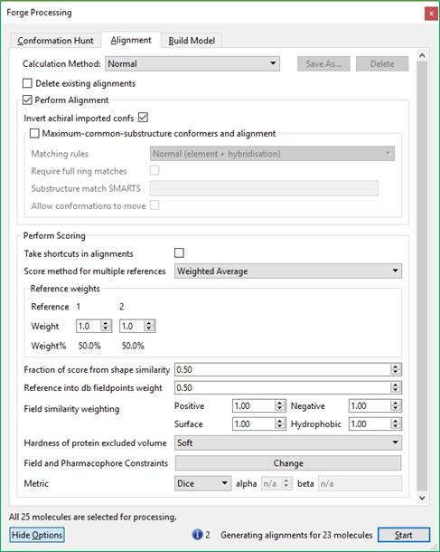
67 67 / 204

68 The 'Normal' alignment uses the standard Cresset alignment method, based on the field point overlay technique. Note that the Reference weights' section only appears if you have loaded more than one reference molecule into Forge, and is only enabled for the Weighted Average' method of scoring for multiple reference molecules. The available setti ngs are explained below. Note that holding the mouse above any value will show a pop-up that gives a quick summary of that option. Option Meaning Invert achiral imported conformations If this option is set, the alignment process is allowed to invert achiral molecules whose conformations have been imported. This option must be set is the imported conformations were exported from Forge, as Forge conformer populations filter out mirror-image conformations. Turn this off if you have loaded specific conformations and you do not wish Forge to be able to invert them to get a better score. Chiral molecules are never inverted. Take shortcuts in alignments If this option is set some shortcuts are taken in the pairwise alignment. In practical terms this means that the alignment step is faster but individual alignments will not be optimised and there is a small chance that a good alignment might be missed. Score method for multiple references This option only has an effect when there are two or more reference molecules. With multiple reference molecules, the alignments are scored against each of the references. These score are then combined in a way that is controlled by this option either the average of the scores is taken or simply the highest possible score can be taken forward. In essence, in Maximum' mode the alignment tries to match the single most similar reference molecule, ignoring the others, while in Average' mode the alignment tries to match all of the references simultaneously and averaging the obtained scores. Reference weights If you have multiple references and the score method is set to Weighted Average mode, then you can set the relative weight of each reference molecule here. Note that the weights are part of the project, and do not get saved with any custom calculation setti ngs. Fraction of score from shape similarity The standard scoring function in Forge uses 50% field similarity and 50% shape (volume) similarity to derive the overall similarity between any two conformations. This slider allows the user to change this function. On most 68 / 204

69 datasets the default score with 50% shape similarity gives good results. Field similarity weighting Set a weighting scheme for each field type. Hardness of protein excluded volume Choose to make the protein excluded volume Hard, Medium, Soft or View only. Choosing View only' causes the protein to be ignored during the alignment process. The other options give a small penalty for each atom of the ligand that overlaps with a protein atom. With Soft' each protein atom is treated as relatively squashy'. This option works well where you are prepared to accept results that may have some overlap but you want to remove gross clashes with the protein. Choosing Hard gives a much firmer protein and a sizable penalty for any atoms that clash with the protein. Use this option where you want to remove all results that impinge on the protein structure. Field and Pharmacophore constraints Pressing 'Change' opens the Constraints and Field Point Editor to set field and pharmacophore constraints, and define additional field points to be constrained. Metric The metric to use to score the alignments. The default similarity metric in the current and previous versions of Forge is Dice. Tanimoto is monotonic with Dice, so will not change the rank ordering of results, although the similarity values will change. Tversky lets you set up a more substructure-like or superstructure-like alignment. For a substructure-like alignment (i.e aligning molecules which are substructures of the query), use Tversky with alpha=0.05 and beta=0.95. For a superstructure-like alignment (i.e. aligning molecules which are larger than but include the query), use alpha=0.95 and beta=0.05. Substructure alignment 69 / 204

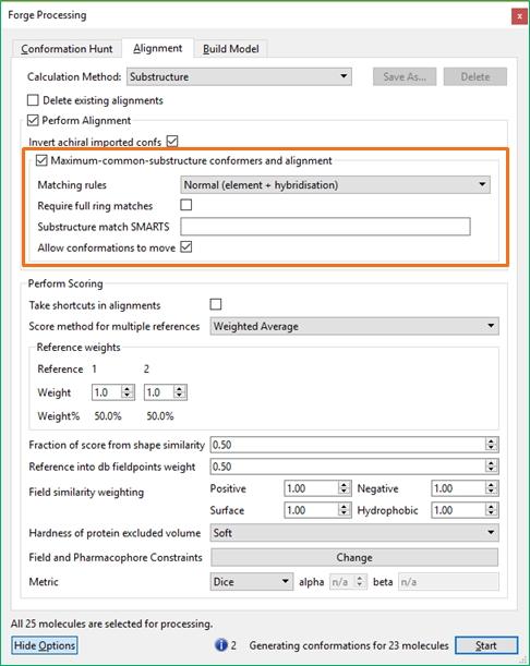
70 70 / 204

71 Choosing the Substructure' alignment setti ngs causes the Maximum common-substructure conformers and alignment' check box to be ticked, enabling the substructure options. Using a substructure based alignment causes a change to both the conformation hunt and alignment stages as part of the conformation hunting process is skipped. Instead of performing a standard conformation hunt and the aligning the conformers, selecting this option aligns all molecules to one of the references according to a Maximum Common Substructure (MCS). A restricted conformation hunt is then performed on the remaining atoms, and the resulting conformers are scored in this aligned orientation. The result is a largely substructure-based alignment of molecules, with the field score used to select orientations for any side chains. Option Meaning Matching rules Set how the MCS is calculated between each molecule and the reference. In 'Normal' mode, atoms match if the elements and the hybridization states are the same, but ring bonds cannot match chain bonds. In 'Permissive' mode, the method ignores element, but matches on atom hybridization. For example, cyclohexane would match morpholine, but not benzene. The 'Very Permissive' mode is like the 'Permissive' mode, but ring atoms can match non-ring atoms. For example, butane can match (part of) cyclohexane. Require full ring matches When in 'Normal' or 'Permissive' mode, disallows partial ring matches for the MCS and forces the MCS to match rings fully. Substructure match SMARTS Specify the substructure you wish to match by writing a SMARTS pattern. When the substructure alignment is performed, substructures matching this SMARTS pattern are strongly preferred. Allow conformations to move After the substructures have been fitted together and the pendant groups have been conformationally sampled, the conformations are permitted to move to give the best score possible, disrupting slightly the substructure alignment but improving the field similarity. Conformation hunt options 71 / 204

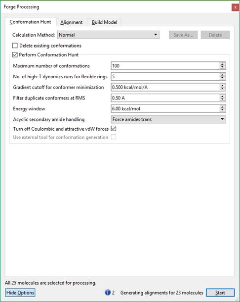
72 72 / 204

73 The available setti ngs are explained in the table below. Note that holding the mouse above any value will show a pop-up that gives a quick summary of that option. The option that has the largest effect is Maximum number of conformations'. More conformations almost always give rise to better alignments, but at the cost of calculation time. Between 50 and 200 conformations are recommended. Very large or very flexible molecule (more than 600 MW or 7 rotatable bonds) will probably require more than 200 conformations to fully explore their conformation space and hence the maximum number of conformations that can be requested is That being said, Forge is optimized for the alignment and conformation exploration of drug-like molecules and thus, is unlikely to give satisfactory results for extremely large and flexible molecules (>12 rotatable bonds) regardless of the number of conformations are requested. If conformations are imported, or molecules are imported in a pre-aligned relationship, the conformation hunt may be skipped. Note also that the Substructure' alignment method has a major impact on the conformation hunt for all molecules which contain a common substructure to the reference molecule. Option Meaning Maximum number of conformations The maximum number of conformations to generate for any molecule. Values of are recommended and a maximum of 1000 can be set. Number of high-t dynamics runs for flexible rings Most small rings are handled using a ring conformation library. Conformations for rings that are not found in the library are sampled using high-temperature (~600K) dynamics with energy initially distributed into torsional degrees of freedom. The number of dynamics runs (and hence the degree of ring conformation sampling) is set by this value. Values of 2-10 are recommended. Values above 5 make little difference to flexible rings of fewer than 8 atoms. Gradient cut-off for conformer minimization All conformers found are minimized using the XED force field. This option sets the gradient cut-off at which the minimization is terminated. Values that are too small lead to insufficient sampling of conformational space and long run times. Values that are too large can lead to unrealistic structures being generated. Values of 0.1 to 1.0 are recommended with values at the smaller end of the range being preferred if the Turn off Coulombic and attractive vdw forces' option is set. Filter duplicate conformers at RMS The similarity threshold below which two conformers are deemed identical. This effectively controls the coarseness of the sampling of conformational space. A low value leads to conformations that are only marginally different, while using a large value means that a conformation near the correct' one may not be 73 / 204

74 generated. Values of 0.5 to 1.0 are recommended: values at the higher end of the range are more appropriate for larger, more flexible molecules. Energy Window Conformations that have a minimized energy that is outside the energy window are discarded. The window is calculated from the lowest energy conformation that has been found. The ideal value for this option depends on the minimization gradient cut off and Turn off Coulombic Forces' options. The best results when the Turn off Coulombic Forces' option is checked are obtained by minimizing to a low gradient (0.1 or better) and applying a smaller energy window (3 kcal/mol) but this significantly increases the time for the calculation. Unchecking the Turn off Coulombic Forces' option requires a significantly larger energy window for large molecules (12kcal/ mol) as these can form very low energy collapsed and internally H-bonded structures. Acyclic secondary amide handling The default setti ng, Force amides trans', forces all acyclic secondary amides to the trans geometry. The Use input amide geometry' sets amides to be not rotatable, but does not coerce them to trans first. As a result, if the input molecule was drawn with a cis amide then only conformations with cis amides will be generated. The Allow amides to spin' sets amide bonds as rotatable so a mixture of cis and trans amides can be generated. Note that this option has no effect on ureas, urethanes, and thioamides as the N-C bonds in these are always treated as rotatable. Turn off Coulombic and attractive vdw forces If selected, long-distance electrostatics and attractive vdw forces are turned off. This generally results in better conformation populations, especially for larger, more flexible molecules. However, for molecules that contain internal hydrogen bonds which strongly constrain their conformations this option should not be used. Use external tool for conformation generation This option only appears if you have set up an external conformation generator in Forge Calculations preferences. Checking this box enables the use of an alternative binary for conformation hunting. The conformation population generated for each molecule can be further inspected and analyzed using the Conformation Explorer. 74 / 204

75 Build Model options The available setti ngs are explained in the following sections. Note that holding the mouse above any value will show a tooltip that gives a quick summary of that option. NB: The Training Set' role must contain molecules for the model building option to be available. There are three types of models that may be calculated from the Build Model panel, based on the type of QSAR desired: Field QSAR, Activity Atlas, and knn (k-nearest Neighbor). Each of these models has their own calculation parameters, described in the sections below. Field QSAR model options The preset calculation methods encompass three different Field QSAR model building experiments: Fast - calculates a model but omits the compute intensive randomization of activity data (y- 75 / 204

76 scrambles). Normal - creates a standard model where all molecules in the training set are weighted equally and validates this using a leave-one-out (LOO) measure of q2 and fifty Y-scrambles. Weighted - uses the reported similarity score of each molecule in the training set to the reference molecules to weight the contribution of the molecule to the model using a linear model. It uses LOO validation and fifty Y-scrambles. This method provides a way to automate model building by considering the similarity score as a measure of how much the alignment should be trusted. For a description of the underlying principles of Field QSAR models please see the Generating Field QSAR models and 3D-QSAR sections. Field QSAR Option Meaning Maximum number of components The maximum number of components to extract from the PLS regression. The default of 20 should rarely need to be changed. Sample point minimum distance This option controls the sphere exclusion algorithm used to reduce the initial number of field sample positions down to a smaller set. A value of 1Å means that sample points must be at least 1Å apart from each other. Reducing this value increases the number of sample points, which may improve the model at the expense of increasing the likelihood of over-fitti ng. Generate samples from references If this option is selected, the field points of the reference molecule(s) will be included in the set of field sample positions to consider. The default is to use only the field points of the Training Set molecules. Number of Y scrambles In each scramble the activity values are randomly assigned to molecules and the model building process is repeated. More scramble sets provide stronger confirmation of statistical significance, but take longer to calculate. Fields to use The default is to build a model from both electrostatic and volume fields, but if desired you can use just one of these. Weight molecules by similarity If turned on, the contribution of each molecule to the model is weighted according to its alignment similarity. Weight ramp type This controls how the weights are ramped between the minimum and maximum similarity values. For example, if the minimum is set to 0.4 and the maximum to 0.8, the weights are calculated as follows: Similarity Weight - Linear Weight - Quadratic > (0.752) (0.252) < Maximum similarity The similarity value above which a molecule gets a weight of 1.0 Minimum similarity The similarity value below which a molecule gets a weight of / 204

77 Cross-validation type During validation of the QSAR model the method used to test the robustness of the model can be Leave-one-out: the model is built again but a single molecule left out of the process, this is then repeated leaving out each training set molecule in turn. The predicted activity for each molecule is the value obtained when it was left out of the model building process. Leave-many-out: the model is built multiple times (specified by the Repeats' parameter) leaving out a proportion of the data (specified by the Training set to use as validation data' parameter). The predicted activity for each molecule is the average of the predicted activities obtained for each model for which the molecule was left out. Training set to use as validation data Percentage of the molecules to leave out in each repeat of the leave-manyout cross validation. Repeats The number of times the leave-many-out validation is run. Larger numbers give more reliable results. Activity Atlas model options 77 / 204

78 Activity Atlas models use a Bayesian analysis of active and inactive molecules to create probability based models of activity. The final models are highly visual, providing information about active molecules, critical regions of SAR and explored regions around your molecules. However Activity Atlas models are qualitative only - they do not make predictions for new molecules. The options associated with the Activity Atlas calculation are presented in the table below. For a description of the underlying principles of Activity Atlas models please see Generating Activity Atlas models. Note that Activity Atlas models are built from the Training Set molecules only and do not use Test Set molecules in any way. Activity Atlas Option Meaning Grid spacing The grid size to use for the analysis. A smaller grid gives finer details, but at the expense of longer calculation time. Automatically calculate disparity range When turned on, the disparity range is determined automatically from the Training Set. 78 / 204

79 When turned off, the user can enter a custom disparity range such that pairs with disparity below the minimum are excluded from the calculation, while pairs with disparity exceeding the maximum are treated as though they have the maximum disparity value. Automatically calculate the activity range When turned on, the activity range is determined automatically from the Training Set. When turned off, the user can enter a custom activity range such that each molecule has a calculated weight, based on its activity. Molecules with activities less than the minimum get a weight of 0 ( inactive'); molecules with activities greater than the maximum get a weight of 1 ( fully active'). Automatically calculate the similarity range When turned on, the similarity range is determined automatically from the Training Set. When turned off, the user can enter a custom similarity range such that molecules with alignment (similarity) scores below the minimum are discarded from the model build; those with similarity scores greater than the maximum are considered correctly aligned; those with alignment scores in between are subjected to linear scaling. Molecules required to fully explore a region The number of molecules whose fields must be seen in a 3D region of space before that region is considered fully explored. Fraction of similarity from shape The default is to use 50% shape / 50% fields. Only use one alignment per molecule If turned ON, if there is no preferred alignment set for that molecule, only the best scoring alignment will be used, otherwise, a preferred alignment will be used if available. If turned OFF, if an alignment is designed as preferred', only that alignment is used. Otherwise, all alignments will be used, with relative weights depending on the delta score to the top-scoring alignments. Optimize pairwise alignments If turned on, the relative orientation of each pair of conformers is optimized by means of a simplex optimizer which rigidly rotates and translates one conformer with respect to maximize the similarity score. If turned off, the similarity value is computed from fixed input orientations. Turning this option reduces alignment noise, at 79 / 204

80 the expense of computational cost/time. Force the use of distance-dependent dielectric By default, this option is turned on. Based on internal testing, Activity Atlas performs best when a distance-dependent dielectric is used. It is recommended that you leave this option checked. k-nearest Neighbor model options knn is a well-established QSAR approach for predicting the activity of new molecules by extrapolating the activity of a number of similar molecules. In Forge the knn algorithm can take use either 3D field similarity or a range of 2D similarity techniques to measure the distance between molecules. The options associated with the k-nearest Neighbor calculation are presented in the table below. In common with Field QSAR methods, the knn method creates a model based on the molecules in the Training Set and predicts the activity of 80 / 204

81 all other molecules in the project, reporting the statistics for those in the Test Set. For a description of the underlying principles of knn models please see Generating knn models. knn Option Meaning Maximum number of K neighbors Maximum number of neighbors to consider Similarity Type The options include Field (Cresset calculated) and a number of 2D Fingerprint metrics. Fraction of similarity from shape The default is to use 50% shape / 50% fields. Optimize pairwise alignments If turned on, the relative orientation of each pair of conformers is optimized by means of a simplex optimizer which rigidly rotates and translates one conformer with respect to maximize the similarity score. If turned off, the similarity value is computed from fixed input orientations. Turning this option reduces alignment noise, at the expense of computational cost/time. Weighting scheme The weighting method to use when averaging the activities of the closest neighbors. In 'Automatic' mode, all the weighting options are tried and the one that provides the best q2 value is chosen. Molecule Editor The Molecule Editor enables the drawing and editing of new and existing molecules and their alignments. It can be opened from the Edit menu, by double-clicking on a molecule in the Molecules table or Tiles view, or using the right-click menu on the Molecules table or 3D Window, and selecting one of the edit commands. The editor has two modes, Rotate Mode and Select Mode (see below) that change the function of the mouse. Conveniently the Ctrl' key can be used to temporarily switch between modes enabling easy access to both rotation and selection. The toolbars can be used to show reference and protein molecules (in the display style that is used for them in the main window) or to display information about the current molecule. The surface fields will automatically update as the conformation of the molecule is changed which can impact the responsiveness of the application. In this case lowering the surface quality in the preferences or turning off surfaces should restore the responsiveness of the application. 81 / 204

82 Molecule Editor quick help Pressing the Help button will show this help. The fastest way to draw a molecule is to quickly sketch the carbon skeleton, then hover the mouse over the heteroatoms and press the element symbol. Quick Help LMB = Left Mouse Button; RMB = Right Mouse button LMB-click an atom/bond to change its type LMB-drag an atom to create a new atom or bond LMB-drag a bond to rotate it (press Shift to change end) LMB-drag an atom with Shift held to rotate a selection RMB-drag an atom/bond to move it RMB-click for context menu Ctrl-Z undo Ctrl-Y redo Additional functionality Listed below is the easiest way to accomplish various actions in the editor. Note that many of these actions are also available in a context menu by right-clicking on an atom. 82 / 204

83 Action Key / Button Undo Press Ctrl-Z, or click the 'Undo' icon in the title bar. Redo Press Ctrl-Y, or click the 'Redo' icon in the title bar. Select atoms Ctrl-Click on the atoms, or hold Ctrl and draw a rubber band. Add an atom Click and drag on an existing atom to draw a new one. Change element Hover over an atom and press the key for the new element (e.g. 'F' for fluorine). Change element for multiple atoms Select one or more atoms, then click the element button. Change bond order Click on a bond to increment, or hover over a bond and type '1', '2' or '3'. Twist a bond Click and drag on a bond. By default the larger side will stay still and the smaller side will move: hold the Shift key to reverse this. Move an atom/bond Right-click and drag on the atom/bond. Move a set of atoms Select the atoms, then right-click and drag on one of them. Rotate/translate the whole molecule Hold down the Shift key, then drag the left mouse to rotate and the right mouse to translate. Add a phenyl Select the phenyl fragment. Click on an atom Change it to phenyl, if possible, or add a phenyl if not. Click on a bond Fuse phenyl to this bond, if possible. Drag on an atom Add a phenyl to that atom. Minimize part of a molecule Select the part you want to minimize, and press the 'Minimize' button. Invert a chiral centre Right click on the chiral atom, and choose 'Invert Chirality' (you might need to add hydrogens first). Change the charge of an atom Click the appropriate charge button ('+', '-' or '0') then click the atom. Editor right-click menu There is a right click menu in the editor that is identical in both rotate and select mode. The right click menu has two forms. The shorter form appears when you right click on a white space. 83 / 204

84 The longer form contains all the entries from the shorter form and appears when you right click on an atom in the editor. Entries are listed below with explanations where appropriate: Undo [action] Redo [action] Select All Invert Selection Swap the currently selected atoms with those that are unselected. Select Fragment The parent fragment of the highlighted atom will be selected. Useful for removing portions of a large molecule. Select Waters Only available if the molecule that is being edited includes water molecules (i.e. it is a protein). Copy Selection Copy the selected atom(s) to the clipboard. Cut Selection Remove the selected atom(s) and place a copy on the clipboard. Recenter View Places the molecule being edited at the center of the display rather than centering on the reference molecule. Center View on References/Selection Recenter the view on the specified reference molecule or selection as appropriate. Delete Deletes the selected atom(s) Set Element Change the selected element to the one chosen Charge Make Positive: make the selected atom positively charged (for example if it is a primary amine). A formal charge will be added to the atom and the protonation state altered appropriately. Make Neutral: remove all formal charges on the selected atom Make Negative: make the selected atom negatively charged (for example it is part of a carboxylic acid). Note that the editor will automatically change additional atoms that are part of a resonate structure (such as the other oxygen atom in an acid). Invert Chirality Appears only if the selected atom is chiral and invertible (e.g. is not at a ring bridgehead). 84 / 204

85 Save Image As Save an image of the current 3D window to a file. Rotate mode The Rotate Mode mode is primarily used to draw and edit molecules in the 3D window. Left-clicking on an empty window or on an atom will place the currently selected atom type or ring template in the window at that position. Left-clicking and dragging will draw a new bond to a new atom of the currently selected type. Clicking on an existing bond will increment the bond order of that bond while left clicking and dragging on a bond will cause the lightest end of the bond to rotate (use Shift as a modifier key to rotate the other end). Right-clicking on an atom or bond will bring up a context sensitive menu. Finally, right-clicking and dragging on an atom will move that atom and any attached hydrogens. Mouse button actions are summarized in the table below. Note that using the ring drawing tools and clicking on an atom or bond will sprout a ring at that position but that it is not always possible for the application to determine what you intended. In these cases, nothing will be drawn and you will have to draw the ring manually using the appropriate element tools. The editor has an extensive set of keyboard shortcuts that make drawing molecules more efficient. For example most elements can be placed by hovering the mouse over an atom and typing a letter (n for nitrogen, c for carbon etc). Equally bond orders can be set by hovering the mouse and typing a number (1, 2,or 3) and atoms can be removed by hovering and pressing the Delete' key. A full list of shortcuts is given in the Appendices. A list of actions and common key presses is given in the table below. Action Mouse (+Key) Rotate all objects Left-click on white space and drag Change element for one atom Left-click on the atom with correct element selected in drawing widget OR Hover over the atom, and press the appropriate letter ( c'=carbon, o'=oxygen, etc.) Grow a ring at this point Left-click on an atom with ring selected in drawing widget Sprout a new atom or ring using the currently selected element or ring Left-click on an atom and drag Increase bond order or grow current ring from this bond Left-click on a bond Move selected atom Right-click and drag on an atom Rotate lightest end of bond Left-click and drag on a bond Rotate heaviest end of bond Press Shift, left-click and drag a bond Rotate molecule relative to reference and/or protein Press Shift, left-click and drag on white space Translate molecule relative to reference or protein Press Shift, right-click and drag on white space 85 / 204

86 Translate a selection of a molecule Select the piece to be translated using Select mode', press Shift, right-click and drag on any atom in the selection Display right-click menu Right-click on a white space Display long right-click menu Right-click on an atom Z-clip the display Press Ctrl, right-click and drag up or down Select mode Choosing Select Mode, either using the radio button on the Select/Rotate widget or by pressing and holding the Ctrl key, changes the function of the left mouse click to enable selecting of atoms or portions of molecules (by drawing a lasso). Once atoms have been selected, the functions of both the Drawing Widget and the Actions Widget apply only to the selected atoms. In this way, it is possible to minimize just a portion of the molecule being edited. Molecular Editor widget and toolbars 86 / 204

87 The Drawing widget is used to select the current drawing tool (element, ring, etc.). Note that most of the elements and charge buttons have keyboard shortcuts so that hovering over an atom and typing o' on the keyboard will convert the atom under the cursor to an oxygen atom. Similarly, typing +' will add a formal charge to the atom and 0' will remove the formal charge. The Actions widget is used to: Control the correct addition of hydrogens (Add H button) Calculate the charge for the molecule using Cresset rules (Charge for ph7) Add fields to a specific conformation of the molecule (Add Fields) Minimize the energy of the molecule to the nearest local minima as a stand-alone molecule (Minimize). The minimize function is useful in setti ng up specific ring conformations (which can be held through the conformation hunt by setti ng dynamics to zero) and for cleaning up newly drawn structures to sensible bond lengths and angles. The Optimize Alignment button will align the current conformation of the molecule to the stored reference molecule using fields and the score for the alignment will appear in the Score information' section located below the bottom left-hand corner of the 3D window of the Molecule Editor. If you have a QSAR model pre-calculated then the score against this model will also be displayed. Pressing Save a Copy will save a copy of the molecule (in its current state) to the Forge project, without exiting the Molecule Editor so that you can continue with your editing. The Information widget provides an interface for naming new molecules and for recording any thoughts or deliberations in the editing or the design of new compounds. When the Molecule Editor is closed the Title text will be returned to the Title column in the main project while the Notes will be transferred to the Notes' column in the Molecules table or Tiles view. The Radial plot widget shows a radial plot (as currently set up in the main Forge project: see Radial Plot Properties for information about setti ng up a radial plot profile) for the molecule being edited, which will be updated on the fly as you make changes to your design. Please note that properties calculated using a REST interface or a column script will not be displayed in the radial plot within the Molecule Editor. 87 / 204

88 The toolbars in the Molecule Editor can be used to undo/redo actions, show reference and protein molecules (in the current display style in the main window), to display information about the current molecule, or to graphically display any models calculated. The field surfaces will automatically update as the conformation of the molecule is changed which can impact the responsiveness of the application. In this case lowering the surface quality in the preferences or turning off surfaces should restore the responsiveness of the application. 88 / 204

89 Saving your changes There are three buttons available to you when you have finished editing. The Align' button appears only if you are editing a database molecule and the current project has at least one reference molecule. Action Mouse (+Key) OK (no references) Save the edited molecule OK (with references) Save the edited molecule in the current alignment: do not generate conformations or re-align. Use this option if you are using the editor to tweak existing alignments. Align Save the edited molecule and bring up the Forge processing dialog for it. Use this option if you have changed the structure of the molecule and need to generate conformations and align it. Cancel Cancel out of the editor all of your changes are discarded. Activity & Model Manager The Activity & Model Manager is used to specify which data is used as activity information, the error on that activity and also to control the any (Q)SAR models built against the specified activities. It is accessible from the Project menu in the main application, the Processing Dialog in the main application, the right-click menu on the column headers of the Molecules table and from the Setti ngs 89 / 204

90 menu in Activity Miner. Note that the manager is not accessible while calculations are being performed. Key Concepts Forge has one special activity category: Primary'. This activity is used to calculate key physicochemical properties such as ligand efficiency for all the molecules in the table. The primary activity will default to the first one in the Activity and Model Manager window but any activity can be set as primary by clicking the appropriate radio button. The columns containing data related to the primary activity are colored pale blue (by default) unless the option 'Color Table by Radial Plot' is set in the Table preferences. Interacting with the Activity and Model Manager The functionality of the Activity Manager window is largely self-explanatory. Each activity is loaded from a column in the Molecules table. For each activity an average error can be specified that controls the treatment of activities within the Activity Miner module. The Units column controls the treatment of the activity value in the Molecules table. The values in the table will be converted to a log scale using this column as a guide. Categorical data requires conversion to a simple numerical scale. When this type of unit is selected, a conversion window pops up (below) that maps Categories to numbers. Alternatively, the Columns Script Editor can be used to create a new column with a conversion of categories into numbers. The description in the Scripts Editor window includes an example of how to accomplish this. 90 / 204

91 Column Script Editor The Column Script Editor is a simple, programmatic way of creating or modifying values in the Molecules table. It uses a JavaScript syntax operating on key properties of the molecules (like the atoms) and on the column data of the project. It is particularly useful for handling activity data. The Column Script Editor window is opened from the Project menu. It has two areas: the main editor window and an information/help sidebar. The sidebar contains details of all available columns and a selection of common example scripts. All text in the sidebar can be dragged and dropped into the main script editor window. Once scripts are complete they can be exported for use by colleagues. The preferences give access to default scripts that can be made available to all new projects. Example scripts are available from Cresset's website at 91 / 204

92 Interacting with Blaze Forge can connect to a local or remote Blaze virtual screening server such as the one available at This gives the possibility to run new and retrieve the results of existing Blaze searches. To use this functionality you must first specify, in the Forge Blaze preferences, the location of the Blaze server that you wish to use together with your username and password on that machine. You can test Blaze by applying for a username on the public demo server at the address above. Running a new Blaze search To run a Blaze search with a ligand or ligand protein pair first ensure the protein is loaded into the Protein' role then select the molecule to be used as a search query. To send the selected molecule to the Blaze server choose the Send to Blaze' option from either the Run menu or one of the right click menus. Note that choosing a reference molecule that has a field and/or a pharmacophore constraint present will cause Blaze to use this constraint in the search algorithm. If the connection to Blaze is successful then Blaze will display the Run Blaze Search' dialog. This gives access to the standard parameters that are used in a Blaze search including choice of collections to search and percentage of results to include in each refinement. See the Blaze manual for detailed information about each of the options. Retrieving results from a Blaze search Once a Blaze search is complete Forge can be used to connect to the server and retrieve the results. To connect to the server and view a list of searches use the Download Blaze Search Results' entry in the File menu. The Blaze Search Results' window will be displayed with a list of all searches that you 92 / 204

93 have permission to view. Check the Show only my searches' check box to view your searches: you can additionally filter them by project using the Only show searches in project' pull down menu. Clicking on a search Name causes the refinements for any search to be shown in the right panel. The right panel gives details on the type of refinement, the number of compounds in the refinement and the status of the search. Generally Cresset recommend retrieving only the results after a simplex refinement has been performed. Results can only be downloaded from refinements that are Complete'. At the bottom of the dialog box are options to control the number of top scoring results to be retrieved and an option to include any protein excluded volume that was used. All downloaded molecules will be added to the Prediction, Reference, and Protein roles as appropriate. Preferences Forge has a number of preferences that can be set from the Preferences panel, launched from Edit Preferences. These are described in detail in the following sections. 93 / 204

94 General Forge has a number of preferences that can be set from the Preferences panel, launched from Edit 94 / 204

95 Preferences. These are described in detail in the following sections. In the General preferences, you have the option to set auto-save conditions and choose whether you want to automatically receive the latest news from Cresset. Appearance The Appearance preferences change the look of Forge and the performance of the 3D display. Most 95 / 204

96 options are self-explanatory or explained using the tooltips. Appearance section 'Application font' sets the font type and size which is used in the Forge interface, e.g., menu text, text on panels and dialog boxes, etc. 3D display section '3D display font' sets the font type and size which are applied to the text that is presented in the 3D window. 'Display quality' sets the overall 3D display quality. 'Surface quality' sets the display quality for surfaces. Surface transparency' controls the degree to which you can see through any surface that is created. Values of 0.3 to 0.5 work well. Note that increased transparency causes an increased graphics workload and hence can slow the performance of the 3D window on some systems. 'Field of View' sets the angular extent of the observable scene in the 3D window. Copy picture resolution' controls the size of the 3D window that is copied to the clipboard. Larger values increase the resolution of the 3D picture on the clipboard giving larger print sizes for publications or posters. Visual scaling of fields' gives you the option to use the size of the point to determine either the radius or area of the point. In the field similarity calculation the field points are used as square root of the size and hence using Area' more closely represents the influence of the point. However, it is easier to see differences between molecules using the default Radius' option. Field color' controls the colors used to display all the field points and field surfaces (negative, positive, surfaces, hydrophobic). Pressing the 'Swap' button swaps the colors set only for the negative and positive field points and surfaces (i.e. starting from the defaults Cresset colors, as you press 'Swap', negative fields will become colored in red and positive fields will become colored in blue). Pressing 'Reset' resets all field colors to the default values. 'Steric coefficients color' sets the color for steric coefficients in Field QSAR models and for hydrophobics and shape surfaces in Activity Atlas activity cliff summary models. 'Electrostatic' and 'Steric variance color' set the color for displaying electrostatic and steric variance in Field QSAR models, respectively. 'Electrostatic' and 'Steric contributions color' set the color for displaying electrostatic and steric contributions in Field QSAR models, respectively. 'Conformation energy gradient' sets the gradient for coloring conformations according to their relative conformational energies in the Conformation Explorer. 'Conformation CSD Torsion Frequencies gradient' sets the the gradient for coloring rotatable bonds according to their calculated CSD torsion frequency in the Conformation Explorer. Max mols to display' controls the maximum number of molecules that will be displayed in the 3D window. The best number depends on the graphics hardware of your machine and should be considered alongside the Display quality' option. Users with fast graphics cards may set this to a large number (>200). By default, you will get a warning should you exceed the maximum number of molecules to display. 'Show max molecules warning': if you uncheck this option, the pop-up warning which appears when you exceed the maximum number of molecules to display will not be shown. Depth cue length' controls the how much fog is used in the 3D window. Larger values give more 96 / 204

97 depth in the view (less fog). Values around 15 work well in most cases. Protein active site size for new projects' sets the radius around the reference molecule that is used when choosing the Only Display Protein Active Site' option from the View menu or the ASite' button on the Protein Display toolbar. Please note that this preference does not apply to the current project but only to new projects. Use the active site radius spin box under the ASite' button on the Protein Display toolbar to change the active site radius for the current project. The Don't show model points smaller than' option controls the display of Field QSAR models in the 3D window. If a Forge Field QSAR model is loaded then this option will disable the display of points that are smaller than the value shown, simplifying the view. Stereo section The Stereo method' choices allow the Forge display to be operated in stereo. Some options may require specialized hardware. The Invert stereo' checkbox reverses the left and right channels. Radial Plot The Radial Plot preferences control the look of the radial plot in the current project. It also sets the default properties and the corresponding parameters that are used in new projects. Radial Plot section The Invert Radial Plot' check box cause the radial plot to operate in reverse of the standard with optimal properties being at the edge of the plot instead of the center. The Center Offset' value is used to move ideal values for a property to be plotted offset from the 97 / 204

98 center by the amount shown in this option. Larger values makes it clearer when non-ideal values are surrounded by ideal properties in the plot. Default Properties section This section provides a set of pre-configured properties which act as a template for new projects and when the property is added to a project. For each property a check box Include by default on new projects' controls whether the property is automatically loaded. Additional properties can be added to this set using box at the top of the Default Property list. The pull down menu allows you to select a property from those available in the Molecules table. If the desired property is not present in the current project, type the exact name of the property. Clicking Add Property' adds the property to the list; the remove button ( ) removes the property from the list. Each property has parameters to set the default function and ranges of values that should be used with the property. Additionally every property has a Weighting that is used in combining properties into a single score that will be presented with the radial plot. Please refer to Radial Plot and MultiParameter Optimization for more details. The remove button ( ) is greyed out for pre-configured properties: these can be removed from the Radial Plot of the current project from the Radial Plot Properties window and prevented from being used in future projects by removing the Include by default in new projects' check and hiding the column in the Molecules table by changing the default columns in the Table section of the Preferences. For each property the default display of the property is set up using the parameter boxes that are shown. Calculations 98 / 204

99 The Calculations preferences control how the application handles aspects of the core science. Conformations section Checking 'Delete unused conformations' will remove all conformations that are not used in the alignments. The removal happens as the last stage of the alignment process so clicking this option on a finished project has no effect. Removing unused conformations drastically reduces the memory usage of the application and is recommended for users operating the 32-bit version of Forge with more than 200 molecules or for projects with large numbers of conformations or when using the Very Accurate' calculation setti ngs. External Conformation Generator section Enables the use of an alternative binary for conformation hunting. Path to binary' specifies the binary that is to be used while the Command-line arguments' are passed as arguments to the binary. Field Points section 'Add Fields' controls the behavior of Forge when molecules are loaded from a file. The Automatically' option causes Forge to convert all molecules to 3D and to add field points to these whenever a molecule is loaded. This works well where smaller a number of molecules is being used. The Manually' option (default) prevents Forge from auto processing molecules after loading, keeping them in the 2D or 3D coordinates that were present in the input source. Fields can be added to all or specific selection of molecules using the entry in the Run menu or by pressing the Add fields' button. This option is best used when operating on large numbers of molecules (>500) that are going to be aligned or otherwise processed within Forge. Force field section 'Force field': Forge is released with the latest version of the XED molecular mechanics force field (XED Force Field 3). To aid compatibility with legacy projects and applications the application can be 99 / 204

100 set to use an earlier version of the force field (XED Force Field 2). The 'Field Calculations' option gives access to an alternative way of handling the dielectric that is used when calculating field patterns and field samples. Instead of a fixed dielectric (2), a dielectric that varies depending on the distance from the probe atom to the observed atom of the molecule is used. The effect is to decrease the effect that formally charged groups exert on a molecule making the charged localized. The effect of this option continues to be an area of active research by Cresset and hence should only be used with caution, unless otherwise specified (please refer to Activity Atlas model options in the Forge processing menu). Similarity Calculations section This preference sets the method that is used for calculating 2D similarities within Forge. Advanced section Checking the 'Show advanced field types' box enables the use of hydrophobic and surface field points in the calculation of FieldQSAR models. In most cases these provide little additional information over the simple volume indicator that is used in standard QSAR model but where you have activities that are very sensitive to the positions of specific methyls or other hydrophobic features then these field types can give superior models at the cost of some interpretability. Processing The Processing preferences will change depending on your Forge license. Using a standard license, this preferences window gives control over the number of local processes to use and the priority 100 / 204

101 with which these should run. With a remote processing license the calculation preferences extend to enable remote processing of the Forge calculations. See the section on Distributing Calculations to learn more about the remote processing capabilities in Forge. Local processing section Set the the number of local processes to use and the priority with which these should run. Extra processing section This section enables the use of a custom FieldEngine binary or more usually a script that can submit FieldEngine processes to a computing cluster. Cresset Engine Broker section Checking the 'Cresset Engine Broker' check box enables the use of Cresset's Engine Broker application that will manage remote calculation resources for Forge. Using the Engine Broker the power of a Linux cluster or cloud computing can be used to accelerate Forge calculations automatically. Remote processing section The location of any remote calculation engines that are available to execute the Forge calculations can be explicitly stated in this section. Table 101 / 204

102 The Table preferences are used to change options related to the Molecules table. Molecules Table section Gives access to the default columns that are displayed in the Molecules table for new projects. These include score columns and activity based columns that only appear once they have values or a primary activity is set in the Activity & Model Manager. Select the columns that should be used by default. The Automatically show and hide columns and radial plot properties..' checkbox causes Forge to automatically show or hide some column properties such as Activity (Primary) and radial plot properties based on project content. The Automatically align the 2D structure of molecules' check box causes Forge to perform a substructure match from each molecule to the references and use this to orientate the 2D layout of the molecules in table to match the reference. The template for the 2D layout functionality can be changed at any time by right clicking on a molecule and selecting Align 2D'. Un-checking the 'Auto-detect activity columns' box prevents activity columns from being automatically added to the Molecules table when molecules are loaded. Properties Radial Plot Coloring' sets the desired color gradient for the radial plots and properties in the Molecules table. Radial plots with overall score of 0 (unacceptable) are colored in red, those with an overall radial plot score of 0.5 (acceptable) are colored in yellow, and those with overall score of / 204

103 (perfect) are colored in green. The same color coding is used to color the property columns. Unacceptable/Acceptable/Perfect colors are set according to the radial plot preferences for that property. Every property that has a profile set in the radial plot preferences is colored in the Molecules table. You can change the default color coding by clicking on the Color' buttons. The Color table by Radial Plot' check box causes Forge to color the radial plot and the cells in the Molecules table by the fit to the radial plot properties. Tile View section Gives access to the default properties that are displayed in the Tiles view for new projects. Note that the Activity (Primary) and LE (Primary) columns only appear once a primary activity is set in the Activity & Model Manager. Select the columns that should be used by default. Default Script Columns section Sets Forge to run the defined script (for example, a new property calculator) for all for new projects. A single script can contain multiple calculations. Import or paste the desired script directly into the column script editor. Alignments section The Maximum alignments per molecule' spin box controls the number of alignments to be displayed in the Molecules table. In most cases, the default value of 10 gives a good balance between the validity of the results and the desire to find an alignment that is different from the top scoring result. Caution is advised when relying on low scoring alignments. Property REST Server section Sets up the URL of an external web services through a REST interface, enabling Forge to incorporate the data computed by such web services in the Molecules table. Please refer to REST interface to external web services for more details about this new functionality. If you need help getti ng your own web service to communicate with Forge, please contact Cresset support. Blaze Forge can be configured with the URL of a Blaze server (Cresset's virtual screening application). Doing so enables the Send to Blaze' and Download Blaze Search Results' options. These enable direct interaction with your local Blaze server or with one of Cresset's Blaze servers. For this option to work correctly you will need both the URL of the Blaze server and your Blaze username and password. From Blaze 10.2 onwards, a fully functional REST interface is used. If you do not know which version of Blaze you are using, please contact your Blaze administrator or contact Cresset support. 103 / 204

104 Activity Miner The Activity Miner preferences govern the setti ngs used when Activity Miner is deployed on a set of molecules. For more information about using Activity Miner for activity cliff analysis, click here. Field Similarity Matrix section 'Fraction of score from shape similarity' controls the field/shape proportion in the score similarity matrix, which is by default, 50/50. Checking the Optimize pairwise alignment' check box causes the alignment of each pair of conformers to be individually optimized from the starting position to maximize the similarity score, at the cost of a longer calculation time. If this box is not checked, the similarity score is computed from the input orientations. Top pairs section 'Minimum Entries to Display' controls the minimum number of pairs that are displayed in the top pairs table. Note that the actual number of pairs that is displayed is half the number of molecules or the value of this setti ng (whichever is larger), plus the number of favorites that have been selected. Activity View section 'Auto Scale entries' controls the number of neighbors that are displayed in the activity view circle when the Auto-scale' option is enabled. 'Maximum Entries' option controls the maximum number of pairs that can be displayed in the circle. 3D View section 'Focus color': this option controls the default color of the carbon atoms of the focus compound in the 3D window of Activity Miner. FieldTemplater 104 / 204

105 FieldTemplater preferences are used to control the display of scores for the templates in the results table of the module. Drag and drop to rearrange, hide or show columns. 105 / 204

106 Conformation Explorer The conformation explorer is a tool to inspect and analyze conformation populations. To open the Conformation Explorer for selected molecules with existing conformations in a Forge or FieldTemplater project, click on the 'Conf Ex' icon in the Analysis toolbar, or right-click on the selected molecules and choose 'Open Molecules in Conformation Explorer' (this functionality is also available from the Edit menu). Separate Conformation Explorer windows will open for each selected molecule with existing conformation populations. In the Conformation Explorer, conformations are listed in the Conformations table order of increasing energy from the lowest energy conformation, which is selected by default and shown in the 3D window as you open the Conformation Explorer (see below). By default, conformations are colored by energy, according to a color gradient which is defined in the Forge Appearance preferences (Edit Preferences Appearance). In the Conformations table, you can easily scroll through the list of conformations using the and keyboard keys, or selecting with the mouse the conformation you want to visualize in the 3D window. If you spot any unwanted conformation(s), they can be marked as deleted by selecting them in the Conformations table (Ctrl-click to select multiple conformations) and then pressing the 'Delete' button, or the 'Del' keyboard button. Alternatively, you can mark selected conformations for deletion from the Conformations table by clicking the Deleted check box, or by right-clicking on one of the unwanted conformations and choosing 'Delete Selected'. Conformations marked for deletion will be greyed out in the Conformations table, and you can choose to hide these completely from the Conformations table by setti ng an appropriate filter. If you change your mind about a deleted conformation, just press the 'Delete' button again and the conformation will be no longer marked for deletion. To permanently remove the conformations marked for deletion from the conformation ensemble for 106 / 204

107 that molecule, exit the Conformation Explorer clicking the 'Accept' button (warning: this operation cannot be undone). To exit the Conformation Explorer with no changes, either click the 'Cancel' button or simply close the Conformation Explorer window. Any conformation you particularly like can be promoted to the reference role in the Forge project by clicking on the 'To Ref' button, or right-clicking and choosing 'Promote to Reference'. You will be prompted to decide whether you want to clear or keep any existing alignments in the Forge project. Selected conformations can be exported to a SDF file by clicking the 'Export' button. By picking 3 or more atoms (Ctrl-click on the chosen atoms in the 3D window) and pressing the 'Superpose' button window., you can change the default criteria for superposition of conformations in the 3D Analyzing conformation populations Distances, angles and torsions can be measured for each conformation by picking the corresponding atoms and pressing the 'Monitor' button. A column will be created for that monitor in the Conformations table (see picture below), and the monitor will be shown in the 3D window for the displayed conformation(s). Monitor values can be filtered and plotted as a histogram by using the Filters and Histogram windows within the Conformation Explorer. Monitors can be removed from the Conformations table and the 3D window by right-clicking on the corresponding column header and choosing 'Remove Colum'. Pressing the 'Torsions' button will calculate torsion frequencies for all rotatable bonds in the molecule, according to the Torsion Library method (Schärfer 2013, Guba 2016). The Torsion Library contains hundreds of rules for small molecule conformations which have been derived from the 107 / 204

108 Cambridge Structural Database (CSD) and are curated by molecular design experts. The torsion rules are encoded as SMARTS patterns and categorize rotatable bonds via a traffic light coloring scheme in the original publication. CSD torsion frequencies are useful to highlights cases where the torsion angle in a calculated conformation is not one that is frequently observed in the CSD, and is accordingly a possible reason for concern. In the Conformation Explorer, CSD torsion frequencies for all the dihedrals corresponding to each rotatable bond are calculated and reported in the Conformations table, with the lowest torsion frequency values for each bond (which are a possible reason for concern) shown by default. A list of all the torsion frequency values calculated for that rotatable bond can be displayed by clicking on the small triangle near the conformation number (see below). Hovering with the mouse over a torsion frequency value will show the corresponding SMARTS pattern as a tooltip. As you calculate the torsion frequencies, the default colors for the conformations (by energy) will be updated to 'Color Bonds by CSD Torsion Frequencies'. Non-rotatable bonds will be displayed in grey; rotatable bonds will be colored and labeled according to the corresponding CSD torsion frequency values (see above), using a color gradient defined in the Appearance preferences. Style toolbar The buttons in the Conformation Explorer display toolbar largely reproduce the functionality of the main Forge Style toolbar. Functionality specific to the Conformation Explorer are smart coloring by conformation energy and by CSD torsion frequency, according to a color gradient defined in the Appearance preferences. Filters Filters can be applied to any column in the Conformations table of the Conformation Explorer. 108 / 204

109 For example, as shown in the picture above, you can decide to show in the Conformations table only the conformations which are not already marked for deletion, have an energy lower than 3, have a 'High' CSD torsion frequency for Torsion #2, and fit the specified ranges for the distance, angle and torsion monitors you defined. To add a new filter, choose the corresponding column from the 'Add filter' drop-down menu, or rightclick on the column header and choose 'Add Filter'. To remove a filter, press the the filter criteria. button near Histograms Any numerical columns created in the Conformation Explorer can be plotted as a histogram in the Histogram window. 109 / 204

110 The number of bars or bins' that should be used is a configuration option. Conformation(s) that are currently selected will be highlighted in the plot. Equally clicking on a bar will cause the corresponding conformations to be selected. Conformations which do not pass the user-defined filters will be greyed out in the plot. 110 / 204

111 Activity Miner Activity Miner is designed to enable rapid assessment of the structure-activity and -selectivity relationships around a set of molecules that have been loaded into the application. This will work best when the molecules are part of a congeneric series or share significant amounts of substructure. The selectivity options based on 3D similarity work best where the alignment is consistent between all the targets under study (such as different isoforms of the same protein). You can choose to send all the molecules that are currently loaded into the application or just a subset into Activity Miner. In the absence of activity data, the Activity Miner will present the similarity matrix of compounds. Activities can be specified from the input data using the Activity & Model Manager, accessible from the Setti ngs' in Activity Miner or the Project' menu in the main application. Additionally, for 3D similarity and activity cliff analysis to work correctly the molecules must be aligned before sending them through to Activity Miner. Introduction to Activity Miner Activity Miner uses the principles of activity cliffs' that have received much attention in the literature. Unlike traditional approaches, Activity Miner uses the 3D as well as the 2D similarity of molecules to find the regions of SAR that are important within a specific chemical series. Fundamental to Activity Miner is the concept of disparity'. The disparity between a pair of molecules is calculated as the difference in their activity divided by the distance between them. In Activity Miner the distance between a pair of molecules is found from their similarity where similarity is expressed in 3D or 2D. Disparity = DActivity/ (1-Similarity) High disparity values are obtained where the similarity is high and the difference in activity is large i.e. a small change in the molecule has made a big change in the activity. These high disparity pairs indicate important areas of the SAR landscape. Unlike traditional approaches, Activity Miner uses either the 3D or the 2D similarity of molecules to find the regions of SAR that are important within a specific chemical series. An example is shown below. 111 / 204

112 Molecule pairs that have a low disparity and high similarity define bioisosteres or flat regions in the SAR. These regions can be useful to modify the physicochemical or intellectual properties of our molecules without losing activity. Running Activity Miner To enter Activity Miner, press the Activity Miner button in the Analysis toolbar, or select the molecules that you wish to analyze and then choose Show in Activity Miner' from the right-click menu. Alternatively, choose the Run Activity Miner' / Run Activity Miner on Selected Molecules' option under the Run menu. Please note that unless you have activity data for all the molecules then Activity Miner will only work on the similarity of molecules, not the disparity. To convert the similarity values into disparity, select at least one activity from the Molecules table of Forge by rightclicking on the column header or using the Activity & Model Manager available from the setti ngs of Activity Miner or the Project menu of the main application. The Activity Miner interface Unlike the main Forge interface, Activity Miner focusses not on individual molecules but on pairs of molecules. The disparity and similarity information for each pair in the dataset are presented together with a 3D view of the pair under investigation. There are multiple views of the pairwise disparity data that are usually displayed in a tabbed' relationship next to the 3D window but any view can be moved to be shown alongside another. The views are: Disparity Matrix shows the full matrix of all pairs of compounds, color coded by the chosen activity and disparity or by similarity. This is a good way to get an overview of the data. Top Pairs lists the molecule pairs with the highest disparity for the chosen activity, allowing you to see the molecular changes with the largest influence on this activity. A separate Top Pairs window is created for each activity defined in the Activity & Model Manager. Cluster View displays the molecules using a dendrogram to represent the hierarchical clustering of 112 / 204

113 the molecules using the current similarity metric. If a single activity is selected then the titles of the molecules are colored according to the activity value. Activity View this provides a view of the SAR landscape around one molecule. The molecules that are most similar to the chosen molecule are shown together with their structural differences, their activity, their similarity and their disparity values. The Activity Miner window is shown below with the separate views. Each view is described in more detail in the following sections. Whichever view is used, selecting a pair of molecules causes them to be displayed in the 3D window: either side by side or top and bottom (governed by the Grid View' button and the aspect ratio of the 3D window). Throughout Activity Miner, the first molecule is considered as a focus', and the second molecule as a comparator'. Within Activity Miner any pair of molecules can be marked as a favorite'. This is completely separate to the molecule favorites in the main application window. Favorite pairs are designed to enable bookmarking of specific changes that are meaningful within the dataset under study. Any pair that has been marked as a favorite will appear in the Top Pairs tables. The data behind the each view can be exported in CSV format using the right-click menu. In addition, the right -click menu enables a picture of most views to be copied to the clipboard for use in other applications. Activity Miner toolbars and 3D Window 113 / 204

114 114 / 204

115 The Activity Miner toolbars controls which activities are to be studied, which similarity metric is used to calculate disparity, the color scheme that is used and the display of molecules in the 3D window. Settings The Setti ngs button enables control of the main setti ngs for Activity Miner. Activity Source The first control in Setti ngs' allows you to change which Activity column is used for the disparity calculations. This setti ng can be changed also using the 'Activity Control' buttons on the left side of the 'Activity and Similarity Selection' toolbar (see picture above). Similarity Calculation This control allows you to change which similarity metric is used for the disparity calculations. The options are Field similarity Molecules are compared using field and shape similarity in 3D; by default, this is 50% shape / 50% field similarity; ECFP4 Molecules are compared using 2D fingerprints (the ECFP4 circular fingerprint descriptor); ECFP6 Molecules are compared using 2D fingerprints (the ECFP6 circular fingerprint descriptor); FCFP4 Molecules are compared using 2D pharmacophore fingerprints (the FCFP4 circular fingerprint descriptor); FCFP6 Molecules are compared using 2D pharmacophore fingerprints (the FCFP6 circular fingerprint descriptor). This setti ng can be changed also using the 'Similarity' buttons on the right side of the 'Activity and Similarity Selection' toolbar (see picture above). 115 / 204

116 Activity Manager This menu entry gives access to the Activity & Model Manager. Molecule Name Source This entry controls the label that is used for molecules throughout Activity Miner. By default the molecule title is taken as the identifier for each molecule and is displayed in the Disparity Matrix as the column and row headers. However, any of the other columns in the main Forge Molecules table can be set as the name of the molecules in Activity Miner using this menu entry. Matrix Color The Matrix Color button enables control the color scheme used in different parts of the Activity Miner module. There are three separate color scales that can be altered. The Disparity Color Scheme' is used in to color the disparity value in the disparity matrix, top pairs table and activity view. A simple two color system is used with white representing disparity values close to zero. The Activity Color Scheme' is used to color the names of compounds in the Disparity Matrix and Cluster views when a single activity value is selected with the Activity Control buttons. A color gradient is applied between the selected colors using the shortest path across the color palette. The Similarity Color Scheme' is used when no activities are selected. It is applied to the Activity View and Similarity Matrix. Like the activity color scheme, similarity values are mapped to the shortest gradient between chosen colors. 3D controls Most of the controls of the 3D window are the same as for the main application, in particular, field surfaces can be displayed in two different ways. By default the surface generation is the same as the main window, that is the absolute values of the surface is displayed for each molecule. The Diff' button is used to switch to the alternative mode of surface display. In the field difference mode, the surfaces are displayed as relative values between the pair of molecules on display. For each molecule, the surface is displayed where the value of the field is greater than the corresponding value in the alternative molecule. 116 / 204

117 Thus in the picture, difluorobenzene (right) is more negative than benzene in the region around the edge of the fluorine atoms. Equally this region is more positive in benzene and hence is displayed with a positive surface. Correspondingly the hydrogens that are para to the fluorine atoms in difluorobenzene are more positive than those on benzene and hence are displayed with a positive surface. The benzene protons are still positive in character (i.e. they give rise to positive field points) but less positive than for difluorobenzene and hence do not show any surface. In contrast the ring current gives rise to a stronger negative region on the face of the aromatic for benzene and hence gives a strong negative field difference in the display. Disparity Matrix view The disparity information for all pairs of molecules in the dataset is displayed whenever an activity is selected in the 'Activity and Similarity Selection' toolbar. If no activity is chosen then the Disparity Matrix cannot be calculated and the Similarity Matrix is displayed. Each molecule is represented once in each row and once in each column. The order of the molecule in the table is set using the Order By' button in the top left corner. The default order is based on a clustering of the molecules so that similar molecules lie near each other. With a single activity selected, each cell displays the appropriate disparity value for a pair of molecules, and is color coded. By default green represents a pair where the comparator compound (column) was more active than the focus compound (row). Conversely, red indicates a pair where the focus was more active than the comparator. The stronger the color the larger the activity difference relative to the structural/field difference. When two activities are selected on the 'Activity and Similarity Selection' toolbar, each cell in the disparity matrix is split to display both disparities for the pair of molecules. Selecting further activities causes the cell to split further (below). Clicking on any cell displays both molecules in the 3D window with the row molecule as the focus' and the column molecule as the comparator'. Additionally, the top left corner of each cell displays the whether this pair has been marked as a favorite. Clicking on the star toggles the favorite status. Note that this is for the pair of molecules and hence is displayed twice in the matrix. The matrix can be navigated using the mouse, using the arrow keys, or by clicking and dragging a cell in the view. The view is scaled using the mouse wheel. Clicking on Order By' in the top left hand corner of the table brings up a menu to select the sort method for the molecules in the table. Once favorites have been selected, the favorite status can be 117 / 204

118 used as a sort method for the table with molecules with more favorite tags in their row sorting to the top of the list. Generally the highly colored cells in the matrix indicate regions of interesting SAR and are worth investigating first. The matrix can be filtered by similarity value using the similarity filer slider on the left hand side of the matrix or by entering a value for the filter in the spin box at the top of the slider. Sliding the bar upwards increases the similarity threshold (shown in the spin box) for the data from a pair of molecules to be shown. The disparity data from pairs of molecules that have a similarity below the value of the threshold is greyed out, enabling you to focus on just the most similar molecules in your dataset. The data behind the Disparity Matrix view can be exported in CSV format using the right-click menu. In addition, the right -click menu enables to show any molecule pair of particular interest in the main Forge project. This can be useful, for example, to see how a certain pair sits within a Field QSAR or Activity Atlas model. Top Pairs table Each activity that has been added to the project in the Activity and Model Manager has a Top Pairs table widget in Activity Miner. The table contains all molecule pairs that have a high disparity value for this activity plus any pairs of molecules that have been marked as favorites. By default, the table is sorted on disparity value. However, it can be re-sorted on any of the other columns that are presented, including on favorite status. The table shows the highest activity molecule of each pair in the first column together with its activity, and the lower activity molecule of the pair next to it. Other comparisons between the molecules are shown in the right hand columns such as the difference in activity or ligand efficiency. The columns that are displayed can be controlled by right-clicking on any column header and selecting Manage columns' from the displayed menu. This table is a quick way to find the most interesting SAR and can be exported to CSV (using the right-click mouse menu) for 118 / 204

119 study in other applications. The right-click menu also enables to show any molecule pair of particular interest in the main Forge project, and to remove one or both compounds in the pair from Activity Miner. Activity view This view is used to examine the SAR around a particular focus compound. It is equivalent to exploring a single row of the Disparity Matrix. The current focus compound is displayed in the center of a radial plot. Each of the closest neighbors to the focus compound is displayed around it (where closest is defined by the current similarity metric, which can be modified using the Setti ngs' toolbar button or using the buttons on the 'Activity and Similarity Selection' toolbar). The size of each segment represents the distance between the two molecules, so that highly similar molecules have only a very small segment. Each segment is then colored by the disparity between the pair for the chosen activity. If multiple activities have been selected then the segment is split vertically to display all the disparity values for the pair. Thus, short highly colored segments contain vital SAR information. Hovering the mouse over any structure or segment highlights the molecule name, activities, and the similarity and disparities of this molecule to the focus molecule. 119 / 204

120 Clicking on any molecule will choose it as the comparator molecule, and it will be shown in the 3D window along with the focus. Double-clicking will select that molecule to be the new focus. The entire dataset can thus be easily navigated: you can view the SAR around a compound, decide that one of the other compounds shown is worth investigating, and re-center the plot around that other compound for further analysis. The forward and back buttons allow you to go back to a previous view and then return to your current view easily. The control at the left of the Activity View window allows you to control how many molecules are shown around the focus. By default the closest 10 molecules are shown, but you can set a similarity threshold using the slider or spin box, in which case all molecules which are more similar to the focus than the threshold value will be shown. The data behind the Activity View can be exported in CSV format using the right-click menu, which also enables to show any molecule pair of particular interest in the main Forge project, to remove a comparator compound from Activity Miner, and to save an imagine of the current Activity View. Cluster view The currently selected similarity metric is used to cluster the molecules within Activity Miner and the results are displayed in this view using a dendrogram. If a single activity is selected then each line is color-coded by the activity of the molecule or the average activity of the cluster. Clicking on the name of any compound makes this the comparator molecule in the 3D view (displayed second), doubleclicking the name sets it as the focus compound (displayed first in the 3D window). Hovering the mouse over a name or a line shows either the structure of the molecule or summary of the cluster. Clicking on the padlock symbol locks the 2D structure of a particular molecule visible. 2D displays can be dragged around the window. The mouse wheel is used to zoom the view while the view is translated using a left mouse drag. Molecules that have different activities but belong to the same cluster indicate regions of strong SAR. Exploring the cluster view using activity similarities and differences within a cluster is a useful way to examine your SAR. 120 / 204

121 Right clicking on any line displays a context menu where the members of the cluster can be selected in Forge. This is useful for focusing onto a particular subset of the molecules. The cluster hierarchy can be exported in CSV format using the right-click menu, which also enables to show any molecule of particular interest in the main Forge project, to remove a compound from Activity Miner, and to save an imagine of the cluster hierarchy. By choosing Tag Molecules from the right-click menu, a 'Cluster N' tag will be added to the molecules in the main Forge project based in the specified similarity threshold (any existing 'Cluster N' tag will be overwritten). 121 / 204

122 Field QSAR models Forge can use the electrostatic and shape properties of aligned molecules to develop Quantitative Structure Activity Relationship (QSAR) models. Molecules in the Training Set role are used to derive a set of sampling points around the dataset that can be used to probe any molecule for the electrostatic potential or for the volume taken up by molecules. The sample values are combined using Partial Least Squares (PLS) to derive an equation that describes activity (see 3D-QSAR for more details). This Field QSAR model can help to explain SAR data and with the best models used to predict an activity value for newly designed molecules. However, as for any 3D-QSAR method, getti ng a good Field QSAR is challenging due to the requirements of getti ng good and consistent biological data and then generating the correct alignments for all compounds with the lowest degree of noise. We recommend visual inspection of alignments to ensure that there are no anomalies present and to enable Forge to use the best possible alignment in the model building. Where the calculated alignment is sub-optimal, manual intervention can be used to improve them. This can be careful manual alignment in the molecular editor or by marking an alternative alignment of the molecule as a Preferred', which causes the chosen alignment to be used in model building and scoring. Molecules that do not align well should be removed from the model by moving them to the Prediction Set (right click on the molecule, choose Role Prediction Set, or drag and drop the molecule in the Molecules table). Where a complete series or sub-series does not align well changing the reference molecule that is used can also work. Delete the alignments for the series that has not aligned well (tip: use the filters window to bring the molecules together), add to or change the reference molecule and re-calculate alignments just for those molecules. WARNING: if you wish to avoid biasing your QSAR experiment, you must not use the predicted activities from a previous Field QSAR run to decide which molecules require re-aligning. It is very tempting to run a QSAR, look at the plot of actual vs. predicted activities, re-align the worst-predicted compounds and try again. If you do this, then you can indeed get models with a nice high q2 value, but these models will have little or no predictive power. If an initial Field QSAR run produces a poor q2 and you think that the alignments might be the issue, then the safest course is to delete the model, then inspect the molecules, re-align all those that appear to be poorly aligned without regard to their activity or the performance of the previous model, then regenerate the QSAR model. Where Forge is unable to generate a predictive Field QSAR model there is still value in visually inspecting the high and low actives to look for differences in the field patterns. Often significant differences in the field patterns of these molecules are present even though a linear relationship between the field samples and activity could not be found. Field QSAR Workflow To build a Field QSAR model in Forge you will need multiple molecules (at least compounds) that align well with activity values that cover at least 3 orders of magnitude. A QSAR model is considerably easier to create and understand if it is derived from a single chemical series and activity values cover more than 4 orders of magnitude. The workflow used is outlined below. 122 / 204

123 Building a Field QSAR model To build a Field QSAR model, open the processing dialog by clicking on the Process' button ( ) on the main toolbar, then choose the desired Field QSAR model (either Fast, Normal or Weighted) from the Build Model drop down menu. Only the molecules in the Training Set will be used to build the model, but activity predictions will be made also for the molecules in the Test Set and for all the molecules in other roles. Please refer to the Field QSAR model options section for more details about how to fine-tune Field QSAR model building setti ngs. 123 / 204

124 Viewing Field QSAR model information Forge presents the information from a Field QSAR experiment in the QSAR Model window that only appears when a QSAR model is present or has been calculated. A drop-down menu at the top of the QSAR Model window allows to select the QSAR model of interest and to delete unused/ unsatisfactory models. The five tabs which display a Field QSAR experiment information are shown and summarized below. Activity The activity tab shows a graph of predicted versus observed activity for all database molecules using the selected model. The graph contains separate data series for the Training set, Test set, and Prediction set plus the Training set computed using the chosen cross-validation method. Buttons toggle the display of each of these data series. Points in the Activity tab can be selected by drawing a box around them with the left mouse. This causes the corresponding molecules in the Molecules table to also be selected and if the Selected' button ( ) is pressed then the selected alignments are also shown in the 3D window. Using the Activity tab is a good way to examine specific alignments or sets of alignments for molecules (e.g. all molecules within a specific activity range). Q2 The Q2 visualization tab shows graphs of model performance (q2 and r2) measurements against the number of components in the model together with the currently selected model. By default the application selects the model which corresponds to the first maximum in the q2 graph. To select a model with a different number of components, click on the desired location. RMSE 124 / 204

125 The RMSE tab shows how the Root Mean Square Error (RMSE) changes with the number of components used in the model. Two separate RMSE graphs are shown: RMSE' uses the model derived from the entire training set to calculate the error, RMSEpred' uses the cross-validated predicted values. Like the Q2 tab, the number of components in the current model can be changed by clicking with the left mouse. Log The Log tab contains the log of the selected model including the setti ngs that were used in model building. The text in the window can be selected and copied to the clipboard (right-click) for storing externally or adding to the project notes. The Model statistics' table in the Log tab contains the raw data that was used to construct the graphs in the Q2 and RMSE tabs together with the Kendall's tau coefficient for both the full set of predicted score and the cross-validated predicted scores (labeled Tau-pred). The Cross-validated activity predictions' table in the Log tab contains the cross-validated activity predictions for the training set compounds. 3D View The 3D View tab allows to visualize the Field QSAR model in 3D (see Displaying models and Displaying fit to models paragraphs in the next section). Using and Interpreting QSAR Models Once a model building calculation has completed, Forge will present detailed information on the performance of the model and the setti ngs that were used to create the model in a dedicated tab of the QSAR Model window - the Log' tab. This contains statistics for the performance of the model on the training set, the performance of the model when parts of the training set are removed (crossvalidation), and the performance of the model on the test set and lastly the performance of models that were built based on randomized data. Some of this information is presented graphically in other tabs to enable choosing of the best model to use predictively. The null model If Forge is unable to build a model that reliably correlates the sample values that were collected for the training set molecules with activity then it creates a null model. All molecules are assigned a predicted activity that is equal to the average activity of the training set and hence appear in a straight line in the Activity tab (below). 125 / 204

126 Choosing the model to use Once the PLS calculation has been completed, an important parameter that can be adjusted is the number of PLS components to use. As you add more components, the model will fit the training data better (the r2 will improve), but eventually you will start over-fitti ng (the q2 will get worse). Forge by default chooses the smallest number of components that is locally maximal in q2: i.e. the lowest number of components such that adding another one will decrease the q2. This may not be the best choice in all circumstances. In particular, if decreasing the number of components leads to only a very small drop in q2, then you should do so as it reduces the chances of over-fitti ng to the training data. Plots of the q2 and RMSE against the number of components are shown in the Q2 and RMSE tabs. You can change the number of components used by dragging the marker in these plots. Displaying models Once a Field QSAR model has been calculated, useful information can be gained from viewing it in 3D. To view the model coefficients, press Ctrl-1/Ctrl-2 or check the appropriate check box in the 3D View tab of the QSAR Model window (these commands are also accessible from the Model' button on the Selection toolbar and in the View View Model 3D Plots' menu). This will display a new set of field points in the 3D display, whose meaning is detailed in the table below. It is usually useful to display the model points along with the reference molecules, so that you can see where the points are in space. Field kind Name Meaning Field QSAR Model coefficients. Positive More positive/less negative electrostatic potential leads to higher activity Negative More negative/less positive electrostatic potential leads to higher activity Sterics+ More steric bulk leads to higher activity Sterics- More steric bulk leads to lower activity (excluded Press Ctrl-1 or Ctrl-2 to toggle on/off. 126 / 204

127 region) Field QSAR Model variance. Press Ctrl-Shift-1 or CtrlShift-2 to toggle, or press and hold v' while model coefficients are shown. Electrostatic variance Larger points mean more difference in the electrostatic potential in this position across the training set Steric variance Larger points mean more difference in the steric potential in this position across the training set These 'model coefficient' points show the region where the Field QSAR model thinks the local fields have a strong effect on activity. For example, a large point indicates that the model has found a strong correlation between having a more positive electrostatic field there and higher activity values. Note that 'more positive' can equally well be interpreted as 'less negative' it could mean that putti ng strong H-bond donors in that region improves activity, or could equally well mean that putti ng strong H-bond acceptors there worsens activity. You have to look at the molecules in the data set to tell. One thing to note is that the model can only pick up molecular features that change across the data set. If a particular H-bond donor is critical for activity, but it's on the common scaffold so that all molecules in the data set have it, then the model can't pick up that activity requirement and will probably not have any strong model points in that region. To find out when this might be the case, we provide the capability to view the field variance information. In this view, the field points are sized according to the variance in the training set at that position. Points with low variance mean that the fields in that region were much the same for all of the molecules, so the model has little or no information on the requirements for activity there. The truly important points are those with a high 127 / 204

128 coefficient and a high variance. In the picture below, you can see that the data set has lots of changes around the central phenyl, SO2 and amide, but that all of the molecules were the same around the left-hand phenyl ring. As a result, the model contains no information about what changes to that ring might be beneficial for activity. To assist in viewing the coefficients and the variance together, you can quickly toggle between them. Display the model coefficients, ensure that the mouse focus is in the 3D window, and press and hold v'. Displaying fit to model The other useful view of the model data is the 'fit to model' view. This view shows, for a molecule, how well it fits the model and where the predicted activity values arise. To view this, select a molecule, and press Ctrl-F or check the View Field Contributions to Predicted Activity' check box in the 3D View tab of the QSAR Model window (this command is also accessible from the Model' button on the Selection toolbar and in the View View Model 3D Plots menu). The field points for the selected molecule(s) will be replaced by the following: Field kind Name Meaning Field QSAR: Field contribution to predicted activity. Electrostatics+ The molecule's electrostatic field is increasing predicted activity here Electrostatics- The molecule's electrostatic field is decreasing predicted activity here Press Ctrl-F to toggle on/ off. 128 / 204

129 Sterics+ The molecule's steric potential is increasing predicted activity here (i.e. the steric bulk here is good) Sterics- The molecule's steric potential is decreasing predicted activity here (i.e. the steric bulk here is bad) These 'model coefficient' points show the region where the Field QSAR model thinks the local fields have a strong effect on activity. For example, a large point indicates that the model has found a strong correlation between having a more positive electrostatic field there and higher activity values. Note that 'more positive' can equally well be interpreted as 'less negative' it could mean that putti ng strong H-bond donors in that region improves activity, or could equally well mean that putti ng strong H-bond acceptors there worsens activity. You have to look at the molecules in the data set to tell. This view shows how well each particular molecule fits the model. For example, if the model thinks that strong positive fields in a region increase activity, but the molecule has strong negative fields, then a large point will be shown in that region. Toggling between this view and the model coefficients is useful: you can see what the model thinks the requirements for high activity are, where this molecule is meeting those requirements and 129 / 204

130 where it isn't. This provides valuable guidance on what you might want to change to increase the activity. Using Field QSAR models to predict activity In addition to scoring molecules using field and shape similarity to a reference ligand, Forge can score molecules against a Field QSAR model. The easiest way to score molecules against a pre-build model is to use the wizard, choosing 'Fit Molecules to an Activity Model'. If you choose to do this manually then you should load the Forge model file before loading any molecules, as they will not survive the model loading process. Processing molecules such that they give reliable scores against a Forge Field QSAR model should be achieved using the same setti ngs as were used in the creation of the model. This information should be supplied to you by the colleague who developed the original Forge model. Once molecules have been scored against a Forge model, they gain both a predicted activity value and details on how well they fit the model that has been used. The predicted activity values will be displayed in the column headed Pred'. This column should be displayed automatically but can be enabled at any time using the Show/Hide Columns' entry in the Project menu. You should pay close attention to the values in the 'Dist to Model' column. The values here depend on whether the molecule has any field points that are not near any field points in the training set. Values of 'Excellent' or 'OK' indicate that all or most of the features in the molecule were present in the training set, and hence that the predicted activity has some reliability. Values worse than this indicate that the molecule has field points in places that the model hasn't seen before, and in this case the predicted activities may be completely unreliable. For example, the molecule may extend in a new direction. The model doesn't know anything about the requirements for activity in that region, so may predict a high activity for the molecule. However, if the wall of the active site sits there causing a steric clash, the actual molecule may be completely inactive. Predicted activity and Distance to model values are reported also for the compounds in the training and test set originally used to develop the model. Distinct Predicted activity and Distance to model columns are created for each of the models developed within the same Forge project. Designing molecules to fit the Field QSAR model If you have a Field QSAR model active, then the predicted activity and distance to model values are displayed in the editor. You can use this to design molecules to fit the Field QSAR. As you edit a molecule, press the 'Minimize' and 'Optimize Alignment' buttons in the editor. The new predicted activity will be displayed. You can thus test out ideas for improving the fit of a compound to the model, and get interactive feedback on whether your ideas are working. 130 / 204

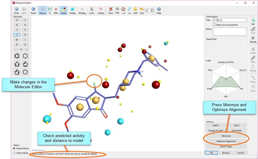
131 131 / 204

132 Activity Atlas models Activity Atlas is a probabilistic method of analyzing the Structure-Activity Relationships (SAR) of a set of aligned compounds as a function of their electrostatic and shape properties. The method uses a Bayesian approach to take a global view of the data in a qualitative manner. Results are displayed using Forge visualization capabilities to gain a better understanding of the electrostatics, hydrophobics and shape features which underlie the SAR of your set of compounds. The Activity Atlas method is designed to be used with data sets of reasonable size (at least 20 compounds) to get a qualitative understanding of the SAR, especially in cases when it is difficult to obtain a predictive Field QSAR model. As with 3D-QSAR, the use of a 3D similarity metric requires the generation of alignments for all compounds and is sensitive to misalignment and alignment noise. The same recommendations about visual inspection and unbiased manual refinement of alignments made for 3D-QSAR apply here (please refer to the Generating 3D-QSAR models section). Activity Atlas carries out three different analysis of the data with the objective of answering the following questions: What do active molecules have in common? Average of Actives What do the activity cliffs tell us about the SAR? Activity Cliff Summary Where have we been? For a new molecule, would making it increase our understanding? Regions explored analysis In calculating the above models, Activity Atlas follows a probabilistic approach which takes into account of the probability that a molecule is correctly aligned (rather than assuming that the top scoring alignment or the selected preferred alignment is the correct alignment), as shown in the picture below. The method starts with the creation of a 3D latti ce of grid points covering the entire volume of the aligned molecules in the data set. For each grid point, and for each active molecule in the data set, different sets of coefficients are then calculated for each Activity Atlas analysis (see Displaying Activity Atlas models for more details). To calculate the coefficients, a weight is associated to each molecule according to an activity range automatically calculated by Forge based on the distribution of activity values in the data set. If the molecule's activity is lower than the low activity threshold (e.g., activity is lower than 6), it is 132 / 204

133 considered inactive. If the molecule's activity is higher than the high activity threshold (e.g., activity is higher than 8), it is considered fully active. If the molecule's activity is between the low and high activity thresholds, then it is partially active and gets an activity weight between 0 and 1 by linear scaling (e.g., if the activity of the molecule is 7, it is given a weight of 0.5). A weight is also associated to each molecule according to a similarity score range automatically calculated by Forge based on the distribution of similarity values in the data set. If the molecule's highest-scoring alignment's similarity is lower than the low similarity threshold (e.g., similarity is lower than 0.6), the molecule's alignment is not trusted, given a molecule weight of 0, and not considered further in the analysis. If the similarity is higher than the high similarity threshold (e.g., similarity score is higher than 0.8), the molecule's alignment is fully trusted and given a molecule weight of 1. If the alignment score is in between, then linear scaling is applied. Note that molecules for which the top scoring alignment is below the low similarity score threshold are disregarded completely. In addition to the per-molecule weighting, Activity Atlas may also considers multiple alignments per molecule and weights them according to their similarity values. The top-scoring alignment gets an alignment weight of 1, and the other alignments get lower weights according to how much lower their score is than the top-scoring alignment. The alignment weights are then normalized so that their sum is 1. For example: The alignment scores for a specific molecule are 0.8, 0.6, 0.5, 0.45: in this case, only the 0.8 alignment will be used with an alignment weight of 1 - the other alignments have much lower scores so get weights of 0. The alignment scores are 0.8, 0.799, 0.798, 0.6: in this case, only the top three alignments will be used with a weight of 1/3 each. Whenever there is a preferred alignment set for a molecule, only that alignment will be used for that molecule and it will get an alignment weight of 1. After computing the molecule and alignment weights, the product of each is used to determine the contribution of each alignment to the final model. This default behavior can be changed to force Activity Atlas to use only one alignment per molecule. In this case only the best scoring alignment (or the preferred alignment if one is set), will be used for that molecule. This implies that you are confident that the best scoring alignment or the preferred alignment is indeed the correct alignment for that molecule. Activity Atlas Workflow To build an Activity Atlas model in Forge you will need multiple molecules (at least 20) that align well with activity values that cover at least 2 orders of magnitude. The workflow used is outlined below: 133 / 204

134 Building an Activity Atlas model To build an Activity Atlas model, open the processing dialog by clicking on the Process' button ( ) on the main toolbar, then choose Activity Atlas' from the Build Model drop down menu. Only the molecules in the Training Set will be used to build the model, but a novelty score will be calculated also for all the other molecules in the project. Please refer to Activity Atlas model options section for more details about how to fine-tune Activity Atlas model building setti ngs. 134 / 204

135 Viewing Activity Atlas model information Forge presents the information from an Activity Atlas experiment in the QSAR Model window that only appears when a QSAR model is present or has been calculated. A drop-down menu at the top of the QSAR Model window allows you to select the QSAR model of interest and to delete unused/ unsatisfactory models. The two tabs which display an Activity Atlas experiment information are shown and summarized below. Activity, Q2 and RMSE tabs Activity Atlas is a qualitative SAR method and accordingly does not have predicted activity, q2 and root mean square error (RMSE) values. Log The Log tab contains the log of the selected model including the setti ngs that were used in model building. The text in the window can be selected and copied to the clipboard (right-click) for storing externally or adding to the project notes. Please refer to the Processing dialog section for more details about how to fine-tune Activity Atlas model building setti ngs. 3D View The 3D View tab allows to visualize the Activity Atlas model (see Displaying Activity Atlas models). Displaying Activity Atlas models Useful qualitative information can be gained from viewing in 3D the results of the Average of Actives, Activity Cliff Summary and Regions Explored analysis, as detailed in the following sections. Average of Actives This model shows you what the average active molecule looks like, by making an analysis of what have in common the active molecules in the data set. To do this, a 3D latti ce of grid points is created, covering the entire volume of the aligned molecules 135 / 204

136 in the data set, and for each grid point, and each active molecule, a coefficient is calculated as follows: Where: Coeff is the coefficient for the grid point Field xyz is the field at this grid point for the active molecule Weight scales the contribution based on the probability that the alignment is correct and the degree of activity. The average of active coefficient for that grid position is then calculated by summing up the coefficients for the active molecules and subtracting the average coefficients for the inactive molecules. The calculation is repeated for all fields (electrostatic, hydrophobic, shape), to calculate the Average Electrostatics of Actives, Average Hydrophobics of Actives and Average Shape of Actives models. To view these models, press Ctrl-1/Ctrl-2/Ctrl-3 or check the appropriate check box in the 3D View tab of the QSAR Model window (these commands are also accessible from the Model' button on the Selection toolbar and in the View View Model 3D Plots menu). This will show a surface in the 3D display, whose meaning is detailed in the table below. It is usually useful to display the surface along with one or more of the most active compounds, so that you can see where the surfaces are in space. Field kind Name Meaning Average Electrostatics of Actives. Average Positive Field of Actives Active molecules in general have a positive field in this region Average Negative Field of Actives Active molecules in general have a negative field in this region Average Hydrophobics of Actives Active molecules in general make hydrophobic interactions in this region Average Shape of Actives Average shape of active molecules Press Ctrl-1 to toggle on/off. Average Hydrophobics of Actives. Press Ctrl-2 to toggle on/off. Average Shape of Actives. Press Ctrl-3 to toggle on/off. The Average Electrostatics of Actives show the regions where, according to the Activity Atlas model, the active molecules in general show either a positive or a negative field. As this field is associated with a high biological activity, new molecules that show either positive or negative fields in the same region (and have the correct shape and hydrophobic interactions) should also be active. The Average Hydrophobics of Actives show the regions where, according to the Activity Atlas model, the active molecules in general make hydrophobic interactions with the target of interest. The Average Shape of Actives shows the average shape of active molecules. 136 / 204

137 Activity Cliffs Summary This analysis is based on activity cliffs (please refer to the Activity Miner and Activity Cliffs sections for more details). To do this, a 3D latti ce of grid points is created, covering the entire volume of the aligned molecules in the data set, and for each grid point, and each pair of molecules, a coefficient is calculated as follows: CoeffAB is the coefficient for this grid point for the pair of molecules AB DisparityAB is the disparity value of the pair of molecules AB MinDisparity is a minimum threshold disparity DField xyz is the field difference at this point for the pair AB Weight is the product of the molecule and alignment weights The coefficients are then added up across all pairs, and the calculation is repeated for all fields (electrostatic, hydrophobic, shape), to calculate the Activity Cliff Summary of Electrostatics, Activity Cliff Summary of Hydrophobics and Activity Cliff Summary of Shape models. To view these models, press Ctrl-4/Ctrl-5/Ctrl-6 or check the appropriate check box in the 3D View tab of the QSAR Model dock (these commands are also accessible from the Model' button on the Selection toolbar and in the View View Model 3D Plots menu). This will show a surface in the 3D 137 / 204

138 display, whose meaning is detailed in the table below. It is usually useful to display the surface along with the aligned compounds, so that you can see where the surfaces are in space. Field kind Name Meaning Activity Cliff Summary of Electrostatics. Positive Electrostatics More positive/less negative electrostatic potential leads to higher activity Press Ctrl-4 to toggle on/off. Negative Electrostatics More negative/less positive electrostatic potential leads to higher activity Activity Cliff Summary of Hydrophobics. Favorable Hydrophobics An hydrophobic interaction in this region leads to higher activity Press Ctrl-5 to toggle on/off. Unfavorable Hydrophobics An hydrophobic interaction in this region leads to lower activity Activity Cliff Summary of Shape. Favorable Shape More steric bulk leads to higher activity Press Ctrl-6 to toggle on/off. Unfavorable Shape More steric bulk leads to lower activity (excluded region) The Activity Cliff Summary of Electrostatics shows the regions where, according to the Activity Atlas model, the comparison of all pair of compounds shows that a more positive field (in the red regions) and/or a more negative field (in the blue regions) increase activity. Note that 'more positive' can equally well be interpreted as 'less negative' it could mean that putti ng strong H-bond donors in that region improves activity, or could equally well mean that putti ng strong H-bond acceptors there worsens activity. You have to look at the molecules in the data set to tell. The Activity Cliff Summary of Hydrophobics shows regions where hydrophobic interaction are either beneficial (green regions) or detrimental (magenta regions) to biological activity. The Activity Cliff Summary of Shape shows regions where steric bulk is either good (green) or bad (magenta). 138 / 204

139 Regions Explored The third and final Activity Atlas model is similar to the Average of Actives analysis, but disregards biological activity completely. Its objective is to make an assessment of what regions of the aligned molecules have been fully explored. At this purpose, a weight is assigned to each field value calculated at each grid point of the 3D latti ce created over all aligned molecules. If the field value is smaller than 2.0, it is given a weight 0 (accordingly, this field value will be disregarded). If the field value is greater than 5.0, it is given a weight 1 (accordingly, the field here is at full strength). In the field value is between the 2.0 and 5.0, it is given a weight which is a linear interpolation between 0 and 1. If more than 10 molecules have a field of strength 5 in a certain grid point position, this position will be considered fully explored. For this reason, meaningless results will be obtained when analysing data sets of less than 10 molecules: all molecules in fact will be classified as fairly novel, as in this case no grid point position can be considered as fully explored. 139 / 204

140 To view the Regions Explored in Negative and Positive Electrostatics, Hydrophobics and Shape, press Ctrl-7/Ctrl-8/Ctrl-9/Ctrl-0 or check the appropriate check box in the 3D View tab of the QSAR Model dock (these commands are also accessible from the Model' button on the Selection toolbar and in the View View Model 3D Plots menu). This will show a surface in the 3D display, whose meaning is detailed in the table below. Field kind Name Meaning Regions Explored Regions Explored in Negative Electrostatics This region in space has been fully explored by negative electrostatics Regions Explored in Positive Electrostatics This region in space has been fully explored by positive electrostatics Regions Explored in Hydrophobics This region in space has been fully explored by hydrophobics Shape Explored Shape fully explored Press Ctrl-7/ Ctrl-8/Ctrl-9/ Ctrl-0 to toggle on/off. It is usually useful to display the model surface along with the aligned compounds, so that you can see where the surfaces are in space. 140 / 204

141 Using Activity Atlas models to calculate a novelty score The Region Explored analysis in Activity Atlas can be used to compute a novelty score for each compound in the data set, as well as for newly designed compounds. In order to do that, Activity Atlas carries out a Region Explored analysis on the training data, repeats the analysis with the training data augmented by the new molecule, and assesses how different are the two models. This means that if a molecule has fields only in places where more than ten molecules in the training set also have strong fields, it has a novelty score of 0, and is labelled as 'Low' in the 'Novelty' column of the Molecules table. Molecules labelled as 'Moderate' add new information to the data set. Molecules labelled as 'Very High' often indicate that the new molecule is overly different to the rest of the data set. Please note that poorly-aligned molecules are classified as 'Low' (as the molecule weight is 0, so it doesn't impact the 'Region Explored' grids) to get a high novelty score, the molecule must have features that haven't been tried before and we must be confident in its alignment. Hovering with the mouse over the Novelty label displays the numerical novelty score associated with that label. Designing molecules with check of novelty score If you have an active Activity Atlas model, then the novelty classification of the compound is 141 / 204

142 displayed in the editor. You can use this to check the novelty of newly designed compounds. As you edit a molecule, press the 'Minimize' and 'Optimize Alignment' buttons in the editor. The novelty classification will be displayed. You can thus test out ideas for novelty, and get interactive feedback on whether you are adding novel chemical information to your data set. 142 / 204

143 knn models As an alternative to Field QSAR, Forge can use the electrostatic and shape properties of aligned molecules to develop QSAR models using the k-nearest Neighbor (knn) method. The knn methodology is a well-known and robust distance learning approach where the activity for each new compound is predicted as follows: A. Calculate the distance (we use 1 - similarity) between the new compound and all the compounds in the training set; B. Select k compounds in the training set most similar to the new compound, according to the distances calculated in step 1; C. Predict the activity of the new compound as the weighted average activity of its k nearest neighbors in the training set. knn QSAR models are a useful alternative to traditional 2D- and 3D-QSAR methods whenever a linear relationship between the descriptors and activity cannot be found. They are particularly useful when developing models for multiple compound series. knn QSAR models can also be useful when working with biological data which are derived from different sources, or when the spread of biological activity is less than optimal (less than three orders of magnitude), such that the standard 3D-QSAR methods are not appropriate. The development of a predictive knn model requires the choice of the most appropriate distance (similarity) metric to use, the optimal number k of neighbors, and the optimal weighting method to use. knn QSAR models in Forge can be built using either 3D (field and shape) and 2D (Fingerprint) similarity. As for 3D-QSAR, the use of a 3D similarity metric requires the generation of correct alignments for all compounds with the lowest possible degree of noise (even though knn is in general less sensitive to alignment noise than PLS). The same recommendations about visual inspection and unbiased manual refinement of alignments made for Field QSAR apply here (please refer to Generating Field QSAR models). The optimal k value in Forge is selected by LOO (Leave-One-Out) cross-validation: each compound in the training set is removed in turn from the modelling and its activity is predicted as the average activity of its k nearest neighbors. These training set predicted activities are used to calculate a q2 value for the model. Different weighting schemes are also applied by Forge to the selected distance metric to assess the statistical performance of the method. The k value and weighting scheme which gives the highest q2 are selected as the optimal conditions for the knn model. Please contact Cresset support for a detailed discussion. knn Workflow The workflow used is outlined below. 143 / 204

144 Building a knn model To build a knn model, open the processing dialog by clicking on the Process' button ( ) on the main toolbar, then choose k-nearest Neighbor (knn)' from the Build Model drop down menu. Only the molecules in the Training Set will be used to build the model, but activity predictions will be made also for the molecules in the Test Set and for all the molecules in other roles. Please refer to the k-nearest Neighbor model options section for more details about how to fine- 144 / 204

145 tune knn model building setti ngs. Viewing knn model information Forge presents the information from a knn QSAR experiment in the QSAR Model window that only appears when a QSAR model is present or has been calculated. A drop-down menu at the top of the QSAR Model window allows to select the QSAR model of interest and to delete unused/ unsatisfactory models. The four tabs which display a knn experiment information are shown and summarized below. Activity The activity tab shows a graph of predicted versus observed activity for all database molecules using the selected model. The graph contain separate data series for the Training set, Test set, and Prediction set. Buttons toggle the display of each of these data series. Points in the Activity graph can be selected by drawing a box around them with the left mouse. This 145 / 204

146 causes the corresponding molecules in the Molecules table to also be selected and if the Selected' button ( ) is pressed then the selected alignments are also shown in the 3D window. Using the Activity graph is a good way to examine specific alignments or sets of alignments for molecules (e.g. all molecules within a specific activity range). Q2 The Q2 visualization tab shows a graph of model performance (q2) measurements against k, the number of nearest neighbors considered in the currently selected model. By default the application selects the model which corresponds to the first maximum in the q2 graph. To select a model with a different k, click on the desired location. RMSE The RMSE tab displays a graph which shows how the predicted (by LOO cross-validation) Root Mean Square Error (RMSEpred) changes with the number of neighbors used in the model. Like the Q2 tab, the number of neighbors in the current model can be changed by clicking with the left mouse. Log The Log tab contains the log of the selected model including the setti ngs that were used in model building. The text in the window can be selected and copied to the clipboard (right-click) for storing externally or adding to the project notes. The Model statistics' table in the Log tab contains the raw data that was used to construct the graphs in the Q2 and RMSE tabs together with the Kendall's tau coefficient for the cross-validated predicted activities (labeled Tau-pred) and information about the weighting scheme used. 3D View There is no 3D View associated with knn models. Understanding Forge knn models Once a model building calculation has completed, Forge will present detailed information on the performance of the model and the setti ngs that were used to create the model in a dedicated tab of the QSAR Model window - the Log' tab. This contains details about the weighting scheme applied to develop the model as well as statistics for the performance of the model on the training set (with predicted activities for the compounds in the training set calculated by LOO). Some of this information is presented graphically in other tabs to enable choosing of the best model to use predictively. The null model If Forge is unable to build a knn model that reliably predicts (by LOO cross-validation) the activities of the training set molecules then it creates a null model. Each molecule is assigned a predicted activity that is equal to the average activity of the training set with that molecule excluded. The predicted activities hence appear in a straight line in the Activity tab (right). Predicted activities for the test set are assigned as the average activity of the training set and also appear as a straight line. 146 / 204

147 Choosing the model to use Once the knn model has been built, an important parameter that can be adjusted is the number of nearest neighbors (k) to use. As you add more neighbors, the model will usually predict the training set activities better (the q2 will improve), but eventually the q2 will get worse. Forge by default chooses the smallest number of nearest neighbors that is locally maximal in q2: i.e. the lowest number of neighbors such that adding another one will decrease the q2. Plots of the q2 and RMSE against the number of nearest neighbors are shown in the Q2 and RMSE tabs. You can change the number of neighbors used by dragging the marker in these plots. Using knn models to predict activity The knn QSAR model can be used in Forge to predict the activity of new molecules. The easiest way to score molecules against a pre-built knn model is to use the wizard, choosing 'Fit Molecules to an Activity Model'. If you choose to do this manually then you should load the Forge model file before loading any molecules, as they will not survive the model loading process. If the knn QSAR model was built using 3D Field/Shape similarity, the processing of newly predicted compounds (in terms of conformation hunt and alignment) should be achieved using the same setti ngs as were used in the creation of the model. This information should be supplied to you by the colleague who developed the original Forge model. Once molecules have been scored against a knn Forge model, they gain both a predicted activity value and details on how well they lie within the model space. The predicted activity values will be displayed in the column headed Pred'. This column should be 147 / 204

148 displayed automatically but can be enabled at any time using the Show/Hide Columns' entry in the Project menu. You should pay close attention to the values in the 'Dist to Model' column. The values here depend on whether the new molecule has any close neighbors among the compounds in the training set. Values of 'Excellent', 'Good' or 'OK' indicate that the new molecule has some close neighbors in the training set, and hence that the predicted activity has some reliability. Values worse than this indicate that the molecule has no close neighbors in the training set, and in this case the predicted activities may be completely unreliable. The 'Error' columns provide an estimate of the spread of activities for the k nearest neighbors which were used to calculate the predicted activity. A value of '0' (zero) indicates that all the k nearest neighbors have the same activity, and accordingly the predicted activity value should be accurate. Large values indicate that the spread of activities for the k nearest neighbors was high, and in this case the activity predictions are likely to be less reliable. Predicted activity, Error and Distance to model values are reported also for the compounds in the training and test set originally used to develop the model. Distinct Predicted activity, Error and Distance to model columns are created for each of the models developed within the same Forge project. If you are editing compounds in the Molecule Editor and you have an active knn model, please note that predicted activity, distance to model and error values will not shown in the editor. Calculating the list of all nearest neighbors may take a long time for large data sets, and accordingly it would not be practical to run this calculation every time the molecule is minimized in the editor. If you want to calculate activity predictions for new designs using an active knn model, draw the new molecule in the Molecule Editor, then save it to the Molecules table. 148 / 204

149 FieldTemplater FieldTemplater is a tool for comparing molecules using their electrostatic and hydrophobic fields in order to find common patterns. Unlike the main Forge application, FieldTemplater requires no 3D information; rather it supplies the template or reference that is used in Forge to align a larger dataset. When applied to several structurally-distinct molecules with a common activity, FieldTemplater can determine the bioactive conformations and relative alignments of these molecules without requiring any protein information. Other pharmacophore generation packages simply attempt to generate a very crude idea of what the protein wants in terms of donor points, acceptor points and the like: FieldTemplater attempts to provide a full picture of how the active molecules bind, which features they use, what shape they are, and how different series can be compared. The hypothesis on which FieldTemplater relies is that two molecules which both bind to a common active site tend to make similar interactions with the protein and hence have highly similar field point patterns. FieldTemplater thus searches for common field patterns across the explored conformational space of a set of ligands, looking for commonality. A field pattern which can be generated by multiple independent structurally-distinct molecules is likely to be related to how those compounds bind to a common receptor. Field points are used in the early stages of molecular alignment to give an approximate measure of commonality, which is then optimized using the full field. A set of hypotheses is produced, each of which suggests a bioactive conformation for each of the supplied molecules and presents how those bioactive conformations relate to each other. Each such hypothesis is termed a template'. FieldTemplater takes as input two or more active molecules, either as single 2D or 3D structures or as pre-generated sets of conformations. It is capable of producing templates' containing up to ten molecules but is most conveniently operated on sets of three to five molecules. Testing against known ligand-protein crystal structures has shown that FieldTemplater can reproduce bound conformations for many ligands with high efficiency. The templating process is shown in outline below. The stages are discussed in a little more detail in How it works and the full algorithm is discussed in Generating templates. 149 / 204

150 How it works FieldTemplater works in several stages outlined in below. If the input molecules were loaded as single structures (2D or 3D), they are passed to the conformation hunter to generate a set of diverse conformations (typically ). If the input molecules were loaded as pre-calculated sets of conformations, then those conformations are used directly. The conformations are atom-typed and processed using into Cresset's XED force field and field points are added to each one. Next, each molecule is compared with every other molecule to create duos'. These duos are the primary building block in FieldTemplater. 150 / 204

151 The duos are created in a multi-stage process. In the first stage, the field points of every conformation of the first molecule are compared with those in each conformation of the second molecule. Matching sets of field points are then used to align the molecules and a single-point field similarity score is calculated. The similarity score uses the field-point-on-field scoring algorithm detailed in Fields and field overlays. The third stage is to optimize the best scoring alignments using a simplex minimizer with respect to both field similarity and volume of steric overlap. Each time a particular pairwise alignment is scored the scoring function that is used is governed by the ratio of field to shape based similarity and the pairwise constraints that are specified by the user. If only two molecules are being processed then processing stops at this stage and the best pairwise alignments are displayed. If more than two molecules are given to FieldTemplater, then a pairwise comparison is performed for each pair of molecules. For example, given 4 molecules A, B, C and D, FieldTemplater will create 6 duos: AB, AC, AD, BC, BD, CD. Once all the duos have been calculated then the next stage is entered 151 / 204

152 where duos are combined to give higher order multiple molecule overlays. This process begins by searching for connected sets of conformations in the duos, where each conformation in the set aligns to each other one with high similarity (below). In this process only one conformation is allowed from each molecule and the number of duos examined from each pair of molecules is governed by the number of pairs' configuration option. Note that when there are more than 3 molecules the software searches for links between all possible molecules (6 links for 4 molecules, 10 links for 5, etc.). As more molecules are used the probability of finding a fully-connected set decreases and hence there is a user-definable tolerance for the percentage of links that need to be present before the conformations are templated. Once FieldTemplater finds a suitable set of conformations, the final templating stage is started. First, all the conformations that make up the set are aligned in 3D and the relative orientations set to minimize the RMS angle and translation deviations between the pairwise orientations in the original duos and those in the template. If the angle and translation errors are sufficiently low, the template is optimized in field space to give a final overlay of the conformations. The final alignment is then scored using both field similarity and volume of overlap. This process is repeated for all conformation sets found to give a full list of templates for the input molecules. For a more detailed discussion of the algorithms used see Generating Templates. Choosing molecules to use in FieldTemplater The choice of molecules to use in FieldTemplater has a large effect on the final outcome and hence is critical to success. A number of factors need to be considered when choosing molecules. General FieldTemplater relies on the assumption that the molecules it is aligning all bind to the same target and use a similar set of interactions (i.e., they have the same binding mode). Therefore, you need to 152 / 204

153 choose molecules that are likely to fit this assumption. In particular, if there is evidence that two active molecules have very different binding modes or bind at allosteric sites, then you shouldn't include them in the same templating run. Additionally, there is an assumption that the molecules are of a similar size to each other and so 3 less potent molecules of a similar size may give better templates that three molecules of wildly different sizes. Flexibility The more flexible your molecules are, the greater the range of shapes they can adopt and the harder it will be to find the right' conformation. You are unlikely to find the bioactive conformation in the conformation search for molecules with more than 8 rotatable bonds and thus, FieldTemplater may not be able to find a reasonable solution. As a corollary to this, if your molecules contain flexible side chains that have little influence on activity (e.g., an n-butyl group) then either mutate them to a conformationally rigid structure such as cyclobutyl or truncate or remove them before submitti ng them to FieldTemplater. Note that any pre-existing knowledge can really help. If you know (or can guess) the conformation of part of your molecule, then carrying out a constrained conformation search using that knowledge can allow you to use significantly larger molecules. Activity The third criterion is activity. The more strongly the molecules bind to the active site, the more information they contain about the active site and therefore, the more likely you are to get meaningful answers. However, there is a trade-off against size: given a large and flexible 1nM molecule and a significantly smaller 10nM molecule the second is usually a better choice. If possible, prune off functional groups and side chains that provide only limited or no benefit to activity: this is especially true of functionality that is present largely for non-activity reasons (solubility, DMPK etc.). Given two molecules with roughly the same activity, choose the less polar one preferentially. Often the best molecules to choose are those with the greatest ligand efficiency that are of a similar size. Diversity The fourth criterion is diversity. FieldTemplater relies on the input molecules having different conformational spaces to eliminate conformational freedom and ultimately identify the bioactive conformations. If the input molecules have very similar conformational spaces then there will be multiple solutions with no way to decide between them. In particular, there is usually little benefit in having two molecules from the same series in the inputs, as any conformation that the first molecule can adopt can be matched by the second molecule. The second molecule thus adds no information regarding which conformations are more likely to be the bioactive one. Note that the diversity which FieldTemplater requires doesn't necessarily correlate with the medicinal chemistry concept of a series'. For example, changing the core of a molecule by atom substitution (going from an indole to a benzimidazole core) can sometimes be thought of as changing series, but if the two series have the same attachments in the same positions then as far as FieldTemplater is concerned there is little shape information to be gained by comparing them. Conversely, increasing or decreasing the chain length in the middle of a molecule (truncating a propyl linker to an ethyl linker, or a urea to an amide) is often thought of as working within a series', but including both variants in a FieldTemplater experiment can give valuable information. One common problem is when all of the active molecules that you have available have a common torsion (see below). If, when aligned, the molecules all have a rotatable bond aligned together, then the solution is under-defined with respect to rotations around that bond. In other words, whatever torsion angle the first molecule adopts around that common bond, the other molecules can all adopt the same torsion angle and align with it just as well. A warning sign that this may be an issue is getti ng larger numbers of templates than you might expect: it is often worth inspecting the templates closely to see if this is the issue. Peptides in particular suffer from this problem: if you are aligning sections of backbone then the backbone dihedrals are under-constrained and so no information about them can be gained from the templating process. 153 / 204

154 If this common torsion issue occurs, then you either have to keep in mind that the solutions are under-defined, or you need to find a molecule which does not share that common torsion and add it to the system. Chain-shortened or -lengthened variants are often useful for this. Number and size of molecules FieldTemplater works best with three to five molecules. There are too many chance alignments between two molecules and so you will tend to get lots of wrong' answers along with the right' answer. Beyond five molecules the calculations can get unacceptably slow and the chance that the software will actually find a template containing all of the molecules becomes low. You are limited to a maximum of 10 molecules in FieldTemplater. Molecules of a similar size give the best results. FieldTemplater assumes that all given molecules bind within the same site and that their bound conformations occupy roughly the same volume. If one molecule is significantly larger than the others, then no information can be gained about the regions of that molecule which do not overlap with the other molecules (the search for a template is under-determined). The conformational noise' in this case makes it difficult to find useful templates. Dealing with uncertain structures racemates, protomers and tautomers Where the exact nature of the binding structure is unknown, perhaps because it has only been prepared as a racemate or because it can exist in multiple tautomeric or protomeric structures, consider combining the different structures into a single entry using the Isomers' feature. In this scenario draw all the possible structures and save them to a single file. If you load these into Forge or create them with the Forge molecule editor then the molecules can be transferred to FieldTemplater as isomers by dragging onto an existing molecule in FieldTemplater. Alternatively load the molecules into FieldTemplater with the File menu Add molecules option and choose the multiple isomer' setti ng in the dialog box. Isomers are treated as separate entities for conformation sampling but will be combined into a single set of conformations for templating. FieldTemplater will automatically select the isomer that templates with the other molecules and display this solution. Note that each isomer gets its own set of conformations according to the limits set in the processing dialog so a molecule with 8 isomers and setti ng of max. 200 conformations for each isomer will result in an extremely long run time. Running FieldTemplater 154 / 204

155 FieldTemplater can be launched via the Forge wizard by pressing, or by selecting molecules within the Forge interface then opening the Run' menu and choosing Run FieldTemplater on Selected Molecules'. Similarly, selecting molecules in the Molecules table and accessing the right-click menu allows you to Run FieldTemplater on Selected Molecules', or to Copy Selected to FieldTemplater', which copies the selected molecules to an existing project in the FieldTemplater application, without setti ng up or running the calculation. Each FieldTemplater project is identified through a unique name that you provide. A Forge project can contain an unlimited number of FieldTemplater projects. The FieldTemplater interface Unlike Forge, FieldTemplater is designed to operate on molecules when no 3D information is available. All conformations of the molecules are aligned to each other and then the alignments searched for sets of consistent alignments that are combined into templates. The main interface displays the molecules that have been loaded together with alignment information and the resulting templates that have been found from these molecules. The remaining toolbars, widgets and windows are dedicated to investigating the results and then communicating these back to Forge. The main areas are described in detail below. 3D Window and FieldTemplater toolbars The display in the 3D window is controlled by all the features of FieldTemplater. Cresset believes 155 / 204

156 that visual inspection of the 3D alignments is the best way to understand the templates and to choose which one is most likely to be correct and/or useful. The main control for the 3D window is the same as in Forge and the same keyboard shortcuts are used. Molecules are displayed using the style that is selected in the Style toolbar and applied to the molecules selected in the Style chooser. Buttons in the Main toolbar are used to return templates to Forge, set pairwise atom constraints, to open the Conformation Explorer and to start the calculation using the processing dialog. The Grid toolbar controls how templates are shown in the 3D window. If the M' grid button is on, then the 3D window is divided into a grid and each molecule is displayed in a separate grid cell. If the T' grid button is on, then the 3D window is divided into a grid and each template is displayed in a separate grid cell. If both are on, then each conformer of each template is displayed in a separate grid cell. Molecule list The Molecules list is shown (by default) on the left hand side of the main interface. This list contains all the molecules that have been loaded into FieldTemplater. A molecule can be selected by clicking 156 / 204

157 on it (the selected molecule is highlighted with a blue border). Selecting a molecule in this manner changes the Style chooser to refer to that molecule. For example, to change the first molecule to ball-and-stick display, click on the molecule, then on the Display' icon on the Display toolbar, and choose Ball and Stick' from the list. Next to the 2D display of the molecule is a list of alignments that this molecule has, and a list of properties that were loaded from Forge. To remove molecules from the FieldTemplater module, simply highlight the molecule then select appropriate entry from the Edit Delete menu, or use the right-click pop-up menu. Removing a molecule from a FieldTemplater project removes all of its associated alignments and all of the templates that contain that molecule. To add molecules to the Molecules list, drag them from Forge and drop onto the FieldTemplater window or choose the appropriate menu entry from the right-click menu. Molecules are transferred together with their conformation populations. If you drop a molecule onto an existing molecule in the molecules list then a dialog box appears asking how the new molecule is to be handled (right). Choosing to add the new molecule as an 157 / 204

158 isomer causes FieldTemplater to populate the conformations of each isomer separately but then combine these in alignment calculations. Results window The results window lists all of the templates that have been found. The first few columns correspond to the molecules that were loaded in the order that they were added to the project and are color-coded for ease of identification. The molecule titles are used as headers: hover the mouse over each header to display the full text in a tool tip. The remaining columns show the scores for each template. By default, the Similarity', Field Similarity' and Shape Similarity' columns are shown. More scores are available by changing the FieldTemplater preferences in the main Forge application. Clicking on a score column header sorts the table by that header. Note that the templates are sorted first by number of molecules, then by which molecules are included, and only then by the selected score type. This is because the scores are not strictly comparable between templates containing different molecules. A template is selected by clicking on its row. This will display that template in the 3D window. Multiple templates can be selected by control-clicking or shift-clicking: all of the selected templates will be aligned to the first one selected and displayed either overlaid, or laid out in a grid, depending on whether the grid display' option is selected (see Grid Toolbar). Selected Log window This window displays all the calculation information for the selected item - molecule or template (or the first selected template where multiple are selected). The information is identical to that obtained through the View menu entry. 158 / 204

159 Most of the entries in the log file are self-explanatory but if something is not clear then please contact Cresset support for an explanation. Menus Most of the menu entries are self-explanatory, or duplicate the functions of the toolbar icons which have already been discussed. Selected entries are explained below. File menu Send selected templates to Forge This menu entry duplicates the function of the Send to' button on the Main toolbar. It is the primary method for transferring results back to Forge. After selecting this option, you will be prompted (below) for the molecule role that should be used for the incoming template in Forge. Add Molecule Opens a file browser window to enable the direct transfer of molecules into FieldTemplater. Export The export menu entry enables the export of either the templates that have been produced (as SDF, mol2 or xed files) or the export of data about the templates in comma-separatedvalue (csv) format for analysis in Excel/Spotfire/etc. Export Visible The Export Visible option causes FieldTemplater to write out only the molecules and conformations that are currently displayed in the 3D window. So to export just the conformation of the 1st molecule in the 1st template, highlight the first row in the table and click on the titles on the 2nd and subsequent columns until only the 1st molecule is shown. Now choose Export Visible'. Export Conformations The conformations for the selected molecules (or all molecules) can be exported in SDF, mol2 or xed format. Note that if the Export all conformations' option is selected, each molecule's conformations will be exported to a separate numbered file ( filename.1.sdf', 159 / 204

160 filename.2.sdf' and so on). Clone Project The current project is cloned to a new project. This option is useful whenever you have satisfactory results in FieldTemplater but wish to explore more options to see if they can be improved further or when you wish to explore the templating process with multiple approaches. All the current data in the project is cloned to a new project with a new name that you specify. Save and Close The FieldTemplater module window is closed but all data is retained and will be saved with the main Forge project. The window can be shown again using the Window FieldTemplater menu entry in Forge. Discard and Close The FieldTemplater results are discarded. Care should be taken as this cannot be undone without reverting to an earlier version of the project in Forge with the File menu Restore Previous Project. Edit menu Copy 3D This copies an image of the 3D display window to the clipboard. It can then be pasted into other applications (e.g., MS Word, MS PowerPoint etc.). Copy Conformers Copies the stored conformations for the selected molecule to the clipboard. This is useful for examining or changing the conformations that FieldTemplater should use. Paste molecule from clipboard Molecules can be pasted into FieldTemplater from several chemical drawing packages including ChemDraw and AccelrysDraw. If there are multiple molecules on the clipboard they will be pasted in separately. Paste Molecule as Isomers/Conformations from Clipboard These options are used to paste molecules in the described way. Delete Delete Conformations for Selected Input Molecules The conformations and all alignments for the selected molecule (blue box around 2D structure and listed in the display menu chooser) will be deleted allowing you to recalculate the conformations using alternative setti ngs. Delete Delete All Alignments All pairwise alignments will be deleted from the project, forcing them to be recalculated the next time processing is started. Conformations are retained. Delete Delete Selected templates The templates which are selected in the Results list will be permanently deleted from the project. Delete Delete All Templates All templates will be deleted from the project. 160 / 204

161 Delete Delete All Results All conformations, alignments, and templates will be deleted from the project, forcing a complete recalculation starting with conformation hunting next time processing is started. Note that conformations will be discarded even if they were originally read in from a file or from Forge rather than being calculated internally. Set Pairwise Constraints This entry opens the Pairwise Constraints Editor which allows the user to specify intermolecular constraints between pairs of atoms. Note that adding a pairwise constraint to a pair of molecules will cause any current alignments between those molecules to be deleted. View menu View log for selected molecule A new window is opened containing the log text for the currently-selected molecule. The log text details the conformation hunt process that was performed on that molecule. View log for selected template A new window is opened containing the log text for the currently-selected template. The log text details the alignment and templating processes that generated that template, including all processing options. Display menu Most of the entries in the Display menu duplicate the functionality of buttons on the Style toolbar. Help menu Show manual Shows this manual! The FieldTemplater processing dialog 161 / 204

162 When at least two molecules have been loaded into FieldTemplater and the Process' button ( ) is pressed (or Run Process is selected from the menus) the processing dialog will be displayed. The processing dialog gives a choice of pre-set parameters for how the Conformation Hunt, Alignment and Templating calculations are conducted. Quick (fast but some templates may be missed) Normal (recommended for normal use) Normal (large mols) (more conformations are generated: suitable for molecules with >6 rotatable bonds) Below the three pre-set parameter sets any previously saved setti ngs are presented followed by a [Custom]' setti ng. This corresponds to the last setti ngs that were used. Pressing Show Options' button or the Setti ngs icon near each calculation method opens the FieldTemplater advanced options panel. Pressing the Start' button starts the calculation. The current activity is shown, along with a list of the things to do and an estimated completion time. Note that the completion time is only a crude estimate, as the actual calculation time will depend on the number of conformations and alignments actually found for each molecule. Clicking More' shows the progress for individual tasks with one progress bar displayed for each FieldEngine that FieldTemplater is using. The parameter pre-sets should suffice for most normal uses, but the calculation parameters can be controlled in detail using the advanced options. 162 / 204

163 FieldTemplater advanced options When you click Show Options' in the FieldTemplater Processing dialog, you will see four tabs in an advanced setti ngs window. The contents of these are explained in the following sections. Custom setti ngs can be saved for future use by using the Save setti ngs' button. The new pre-set setti ngs will be added to the bottom of the main setti ngs chooser. For example, select the Quick' setti ngs then within the advanced options change the Number of Conformations' option to 250. Save the new parameter set as Quick250'. For future calculations that require this set of parameters, simply select the Quick250' option in the main chooser without the need to enter the Show Options' panel. Molecules The Molecules tab displays all the molecules that are currently loaded into FieldTemplater. Only the molecules which are checked in this section will be used in the calculation. This allows you to load in more molecules than are actually used in any one calculation (e.g., load in 10 molecules, form templates from two groups of 5). Note that the Save Setti ngs button does not save or restore the values on this tab as they would be meaningless when applied to another project containing different molecules. 163 / 204

164 Conformation hunt options The setti ngs in this tab are explained in the table below. Note that hovering the mouse above any value will show a tooltip giving a quick summary of that option. For a full understanding of the effects of these options please refer to the Generate Conformations section of the chapter 'The science in Forge: Generating templates'. The setti ng that has the largest effect is Maximum number of conformations'. More conformations mean an increased likelihood that the bioactive conformation will be well-approximated by at least one conformation in the set. However, using more conformations also means adding conformations that are not close to the bioactive conformation which act as noise' in the calculations. Additionally if there are too many conformations then the pairwise alignments will take a very long time to complete and it is likely that many more pairwise alignments will have to be used in the templating process. Between 50 and 200 conformations are recommended. For molecules whose conformation space is not sufficiently explored by 200 conformations it becomes difficult to obtain reliable results without adding additional information such as using pairwise constraints. 164 / 204

165 Option Meaning Maximum number of conformations The maximum number of conformations to generate for any molecule. Values of are recommended and a maximum of 1000 can be set. Number of high-t dynamics runs for flexible rings Most small rings are handled using a ring conformation library. Conformations for rings that are not found in the library are sampled using high-temperature (~600K) dynamics with energy initially distributed into torsional degrees of freedom. The number of dynamics runs (and hence the degree of ring conformation sampling) is set by this value. Values of 2-10 are recommended. Values above 5 make little difference to flexible rings of fewer than 8 atoms. Gradient cut-off for conformer minimization All conformers found are minimized using the XED force field. This option sets the gradient cut-off at which the minimization is terminated. Values that are too small lead to insufficient sampling of conformational space and long run times. Values that are too large can lead to unrealistic structures being generated. Values of 0.1 to 1.0 are recommended with values at the smaller end of the range being preferred if the Turn off Coulombic and attractive vdw forces' option is set. Filter duplicate conformers at RMS The similarity threshold below which two conformers are deemed identical. This effectively controls the coarseness of the sampling of conformational space. A low value leads to conformations that are only 165 / 204

166 marginally different, while using a large value means that a conformation near the correct' one may not be generated. Values of 0.5 to 1.0 are recommended: values at the higher end of the range are more appropriate for larger, more flexible molecules. Energy Window Conformations that have a minimized energy that is outside the energy window are discarded. The window is calculated from the lowest energy conformation that has been found. The ideal value for this option depends on the minimization gradient cut off and Turn off Coulombic Forces' options. The best results when the Turn off Coulombic Forces' option is checked are obtained by minimizing to a low gradient (0.1 or better) and applying a smaller energy window (3 kcal/mol) but this significantly increases the time for the calculation. Unchecking the Turn off Coulombic Forces' option requires a significantly larger energy window for large molecules (12kcal/mol) as these can form very low energy collapsed and internally H-bonded structures. Acyclic secondary amide handling The default setti ng, Force amides trans', forces all acyclic secondary amides to the trans geometry. The Use input amide geometry' sets amides to be not rotatable, but does not coerce them to trans first. As a result, if the input molecule was drawn with a cis amide then only conformations with cis amides will be generated. The Allow amides to spin' sets amide bonds as rotatable so a mixture of cis and trans amides can be generated. Note that this option has no effect on ureas, urethanes, and thioamides as the N-C bonds in these are always treated as rotatable. Turn off Coulombic and attractive vdw forces If selected, long-distance electrostatics and attractive vdw forces are turned off. This generally results in better conformation populations, especially for larger, more flexible molecules. However, for molecules that contain internal hydrogen bonds which strongly constrain their conformations this option should not be used. Use external tool for conformation generation This option only appears if you have set up an external conformation generator in Forge Calculations preferences. Checking this box enables the use of an alternative binary for conformation hunting. The conformation population generated for each molecule can be further inspected and analyzed using the Conformation Explorer. Alignment options The alignment options control how the pairwise alignments of molecules and conformations are performed. The options are described in detail in the table below. Note that hovering the mouse 166 / 204

167 over an option gives an explanation of that option as a tooltip. Option Meaning Fraction of score from shape similarity The user can control the ration of field similarity and shape similarity that is used in the pairwise alignments. Traditionally a value of 0.5 (corresponding to 50% field and 50% shape) has given excellent results. A value of zero would give alignments based solely on Fields, a value of 1.0 would give alignments based solely on shape similarity Invert achiral imported confs This option applies only to conformation populations that are imported from a file into FieldTemplater and are achiral molecules. Usually you will want this option on so that the conformation populations of achiral molecules are immediately expanded to include the conformational enantiomer of every entry. This is especially true when using conformation populations generated by Cresset as they usually have conformational enantiomers removed. However, in some circumstances, such as fitti ng together bioactive conformations, this option should be turned off. Take major shortcuts in pairwise alignments The pairwise alignments are normally generated by aligning the field points, and then performing a simplex optimization from these starting positions using the full field scoring function. If this option is selected, the simplex optimization is skipped and just the initial alignments are used. Significantly faster than all other 167 / 204

168 options but at the expense of accuracy and completeness. Take moderate shortcuts in pairwise alignments Use a looser convergence criterion in the simplex optimization of the pairwise alignments, and simplex fewer of them. Gives a significant speed boost, but at a small cost to quality. Add/remove intermolecular constraints Clicking the Edit constraints' button opens the Pairwise Constraints Editor window where intermolecular constraints can be added or removed. Adding constraints can significantly change the pairwise alignments and simplify the problem that FieldTemplater has to solve. Templating options The setti ngs in this tab are explained below. Note that hovering the mouse above any value will show a tool tip giving a quick summary of what the option does. For a full understanding of all these options please see The Science: Generating Templates. The main options that affect the results are the Maximum number of alignments per pair' and the Maximum score delta per pair'. Increasing the values of these options will give more templates (although possibly of lower reliability), decreasing them will give fewer or no templates. Option Meaning Minimum molecules per template The minimum number of molecules required to form a 168 / 204

169 template. With 5 molecules, set this to 5 to only find templates containing 5-molecules. Maximum molecules per template The maximum number of molecules in a template. With 5 molecules, set this to 4 to only find templates with 4 or fewer molecules present. To find all templates with 3 to 5 molecules present, set minimum molecules per template to 3 and maximum molecules per template to 5. Maximum number of comparisons per pair Up to 1000 alignments are generated between each pair of molecules, sorted by score. In general the best results are obtained if only the highest-scoring alignments are used in the templating process. This value controls the maximum number of alignments that will be used from any pair in forming a template. Values of are recommended. Higher values usually give more templates. Maximum score delta per pair As above, except rather than specifying the maximum number of alignments to use for each pair this option specifies the maximum difference in similarity score between the best-scoring alignment and any alignment to be used. For example, with the default value of 0.1, if the best-scoring alignment of molecules A and B has a score of 0.7, then no alignment of A and B with a score less than 0.6 will be used to generate the templates. Again, higher values give more templates. A range of 0.05 to 0.2 is recommended. Minimum link density in a template The minimum fraction of possible pairwise links that must be used in constructing this template. For example, in a 5 molecule template there are 10 pairs of molecules. A template constructed using 8 pairwise alignments (so that 2 pairs were missing') has a density of 0.8, so would not be allowed if this parameter was greater than 0.8. Lower values are recommended for larger sets of molecules (5 or more) where no templates are found. However, please note that templates with a low link density are less reliable. Filter duplicate templates at RMS If two templates containing the same conformers of the same molecules are found, then remove the lowerscoring one if they are closer than this limit. Skip simplex optimization of final templates Don't refine the final templates. Saves time, but the final template alignments and scores are less reliable. Take shortcuts in optimization of final templates Use a looser convergence criterion in the simplex optimizer for the final templates. The final template scores will have additional errors of ±0.01. Pairwise Constraints Editor 169 / 204

170 The Pairwise Constraints Editor can be opened using the Set pairwise constraints' option on the Edit menu; using the Edit constraints' button on the Alignment' tab of the advanced options in the FieldTemplater Processing dialog; or with the Constraints' button on the main toolbar. Setti ng a pairwise constraint using the Pairwise Constraint Editor window significantly affects how a particular pair of molecules align. Constraints are usually used to ensure that a particular pair of atoms are closely aligned in the final templates but can also be used to ensure specific atoms are held apart. Once opened, the Pairwise Constraints Editor window will show a single representation of each molecule that has been loaded into FieldTemplater (note that the conformation that is shown is not necessarily relevant to the final conformation population). The Pairwise Constraints Editor window is controlled using the mouse as described below. Action Effect Left-click and drag Rotate all molecules in their individual 3D boxes. Middle-click and drag or mouse wheel Scale all molecules (up or down) in their individual 3D boxes. Left-click and drag while holding the <Alt> key Left-click on an atom and drag to another atom on another molecule Add a constraint between the two specified atoms. Right-click on an atom with a Remove all constraints from this atom. 170 / 204

171 constraint To add a constraint between a specific pair of atoms, orientate the two molecules so that the required atoms are clearly visible then left-click and drag a constraint between the two atoms, releasing the left mouse button on the target atom. A dialog box will pop up requesting the minimum and maximum distance for the constraint. Note that there is no limit to the number of constraints that can be applied either globally or between specific pairs of molecules. However, a high number of constraints will severely restrict the number of the results that FieldTemplater is capable of returning. Troubleshooting FieldTemplater Long calculation times The clique-matching algorithm used across the set of pairwise alignments is generally very fast, but the problem of finding the best cliques is an 'NP-complete 'one and so in the worst case, the runtime is exponential in the number of molecules. In other words, most of the time it is quick, but in some cases it can take millions of years to complete. There is some checking code in FieldTemplater to detect likely pathological cases and warn on them, but it's not fool proof. In general, the very long run times come from having many alignments referring to the same conformers. This generally occurs when the molecules are fairly rigid and don't actually have that many conformers in the first place. A good solution in this case is to cancel the calculation, reduce the maximum number of pairwise alignments used (e.g., from 100 to 20) or the maximum alignment score delta (both on the Templating options tab in the FieldTemplater advanced options of the processing dialog) and try again. Generating more results In some cases the default experimental conditions produce few or no results. The most likely reason for this is that there was no set of pairwise alignments between all the pairs of molecules that you provided that generated a convincing multi-molecule alignment. To fix this: If you specified a high minimum number of molecules (in the Templating options), then reduce it. If you can't find any 5-molecule templates, then you might want to look at 4molecule or 3-molecule solutions. In the limit, allowing 2-molecule solutions guarantees answers: inspect these to see if there's an obvious reason why the molecules won't form a consensus model. Try increasing the maximum number of alignments used or the maximum alignment 171 / 204

172 score delta (both on the Templating options). If you are templating large numbers of molecules (more than 5), try decreasing the Minimum link density' in the Templating options. Lastly the conformations that you have may not be appropriate. Try clearing all results (under the Edit' menu), increasing the number of conformations or altering the conformation generation parameters, and starting again. If you still find no convincing templates, then it is possible that: your molecules aren't actually all active using the same binding mode; your molecules are too large and flexible for a realistic search of conformation space to occur (more then 7-8 rotatable bonds and your chances of success start decreasing rapidly); or, FieldTemplater just can't find the right answer In all of these cases, the best solution is to try again with some different input molecules, if possible. Generating fewer results A large number of results generally occur because the values you set for the maximum number of alignments used or the maximum alignment score delta (both on the Templating options) are too high; or, the molecules that you specified are insufficiently diverse. If every possible conformation of molecule A can be matched well by a conformation of molecule B (e.g., if they are close congeners) then having A and B in the data set together is pointless and just adds noise; or, you have a common torsion problem so that one or more torsions in the template models are under-constrained; or, one of the molecules has a flexible group that does not overlap with the other molecules: in this case the flexible group is under constrained and you get a family of related templates differing only in the conformation of this group. Choosing a result Unfortunately the top scoring template is not always right. However in most cases if the correct' answer is found it will be close in score to the top-scoring template. The template score is a measure of how similar the molecular fields and shapes of the molecules in the template are. In this respect, it is quite accurate: a template with a high score will have more similar molecular fields between the molecules in the template than a template with a low score. However, as the final template scores are calculated using a simplex optimizer which has a relatively coarse gradient tolerance (to speed up the refinement) the template scores should be treated as though they have errors of at least ±0.01. Additionally, the absolute value of the template scores isn't that informative in isolation. In general, larger more polar molecules tend to give lower scores: a template of 3 small greasy molecules may well give a score of 0.75, but three larger more polar molecules may well only produce templates with a score of 0.5. That doesn't necessarily mean that the former set of templates is more likely to be correct. Note that the template scores aren't strictly comparable between templates containing different molecules. As a result, the template score is only used to rank templates that contain the same molecules. For example, if you are templating four molecules A, B, C, and D, then all ABCD templates will be shown first, then all ABC templates, then all ABD templates, and so on. The ABC templates will be sorted by score, but will always appear in the table between the ABCD results and the ABD 172 / 204

173 results. Seeing double in the results If none of the molecules in the template is chiral, FieldTemplater cannot distinguish between any given answer and its mirror image. As a result, it usually finds both. The results table will be filled with pairs of results. To know which of these is correct information will be required from a chiral molecule either a chiral small molecule with activity, or the protein active site. 173 / 204

174 REST interface to external web services One of the most requested features by users is the ability to include corporate or externallycomputed data for any compound into the molecule table. For example, some users would like to apply their own pka calculation to any newly designed compound. Forge can connect to an external web service through a REST interface to import the external properties and data computed or retrieved by such web services as additional columns in the Molecules table. Once imported, the properties can be used in the Radial Plot, in the Tiles view, and for coloring molecules and table cells. The URL of the web service can be configured in the Property REST Server' section of Forge Table preferences (Edit Preferences Table). Both input and output to/from the web service are in JSON format, and input will be sent using a raw POST HTTP request with the molecule represented as a SMILES string. Input JSON generated by Forge has the following format: { "molecule": { "SMILES": "<a SMILES string>" } } Output JSON from the web service can have either of the following formats: { "molecule-data": { "Property1": "<value for Property1>" "Property2": "<value for Property2>" [ ] "PropertyN": "<value for PropertyN>" } } or { "Property1": "<value for Property1>" "Property2": "<value for Property2>" [ ] "PropertyN": "<value for PropertyN>" } Example External REST Data 174 / 204

175 An example CGI Python script is given below. This web service uses the RDKit to compute the Wildman-Crippen LogP value: #!/usr/bin/env python import sys import json from rdkit import Chem from rdkit.chem import Crippen jsonin = sys.stdin.read() dictin = json.loads(jsonin) smiles = dictin['molecule']['smiles'] mol = Chem.MolFromSmiles(smiles) dictout = {} dictout['crippenlogp'] = round(crippen.mollogp(mol), 3) jsonout = json.dumps(dictout) sys.stdout.write('content-type: text/html\n\n' + jsonout + '\n') Once the script is installed in a working Apache installation configured to use Python CGI scripts and the RDKit, enter the URL of the web service in the 'Property REST Server section' section of Forge Table preferences: Using this service all molecules loaded or created in Forge receive a "CrippenLogP" column populated with values from the webserver. If you need help getti ng your own web service to communicate with Forge, please contact Cresset support. 175 / 204

176 Distributing calculations Forge is a desktop application focused on the greatest accuracy as possible in a reasonable length of time. To keep run times to a minimum Forge is engineered to use up to 16 local CPUs to generate results in parallel. However, in many situations experiments take longer than is desirable, either because greater accuracy is required or because a large number of molecules need to be processed. Under these circumstances Forge can be configured to use extra processing resources to speed up the calculation. To do this Forge must be able to connect to the additional computers and these must be running a FieldEngine process that performs the calculation. There are different ways in which this can be done depending on the computing infrastructure that is available. All options use the Forge Processing preferences to specify how to interact with the remote resources. Script Control This method of communication with the remote calculation resources relies on a custom script that will start the FieldEngine on a remote computer and communicate the location of the resource back to the Forge application. The script is executed once for each Extra process' that is specified in the appropriate box in the Processing preferences. The nature of the script depends heavily on the computing infrastructure that is to be used and hence can be troublesome to get right. Cresset have experience of using this option in different organizations and hence are happy to provide free technical support with getti ng this option working. Contact Cresset support to discuss your situation and requirements. Using the Cresset Engine Broker Interface The Cresset Engine Broker is a command line utility than acts as an intermediary between the Forge application and the FieldEngine processes that perform the calculation. The broker application starts FieldEngines in a way that is specified by a script, for example submitti ng them to a Linux cluster queuing system such as GridEngine, PBS, SLURM or LSF. Once the engines are running, the broker sends the results computed by the remote FieldEngines back to the Forge application. The main advantage of the broker method for speeding up calculations is that the same resources can be used by many different users on many different platforms, enabling the submission of Forge GUI calculations running on Windows or Mac to a Linux cluster. Using the Cresset Engine Broker is straightforward. With an appropriate license a 'Remote processing' section is exposed in the Processing preferences, where the location of the Cresset Engine Broker can be specified. Alternatively, the environment variable CRESSET_BROKER can be used to specify the hostname or IP address and port that is to be used (syntax is CRESSET_BROKER=hostname:port). Using an explicit connection to remote FieldEngines This option uses FieldEngine processes that have been explicitly started on a specific machine and port. The relevant section in the Forge Processing preferences is then used to specify the location of the specific machine(s). To use this feature you must know which machine and port is hosting the FieldEngine process. Additionally, the FieldEngine must be able to pass data through any local firewalls. To specify the location of a remote FieldEngine, simply type into the 'Remote processing' section in the Processing preferences the name or IP address of the remote machine together with the port which should be used to contact it. For example, a FieldEngine could be started on machine Ganymede' running on port 4000 with the command: nohup FieldEngine p > fieldengine.out 2> fieldengine.log & 176 / 204

177 To connect to this FieldEngine from Forge enter the following in the remote processing box: Ganymede:4000 To facilitate adding large batches of FieldEngine locations the Add ranges' button gives access to the Set a range of hosts' utility that will accept wildcard expressions. Simply type your expression into the box and click the Add range' button. The expression takes ranges of numbers in square brackets, such that cressfarm[31-40]:[ ] would enumerate 40 FieldEngine addresses, 4 processes on each of 10 machines running on ports 4001 to The machines can be specified by hostname or IP address. Once you have enumerated the range of machines/ports that you wish to use, click OK' to add them to the global list. The list of machine names is expanded at the point that a calculation is started, and is not revisited during the calculation; therefore, adding machines to the list to while a calculation is running will have no effect. 177 / 204

178 The science The following sections provide additional details and background information about the science methods available in Forge. Fields and field overlays It is well known that molecules from different structural classes can act at the same biological site. It is also accepted that molecular recognition occurs via electronic and surface properties: electrostatic and van der Waals forces. It therefore follows that if two molecules with different structures interact with an enzyme or receptor at the same site in a similar manner, they will have similar surface and electrostatic properties in their bound conformations. When undertaking molecule design, it is therefore desirable to have a set of molecular descriptors that encode the aspects of a molecule which define its binding interactions. Such a set of descriptors would encode the surface, shape, electrostatic, and van der Waals properties of a molecule rather than its chemical connectivity. In other words, the descriptors would encode the molecular fields on and around the surface of the molecule, rather than a set of atoms and bonds. Field points A full surface description of a molecule over all of its accessible conformations is too complex to handle. The potential fields are continuous functions with complicated formulae. Approximations based on grids or surfaces produce too many data points for fast processing or are restricted in their accuracy by the grid resolution and lack of gauge invariance. Describing fields in terms of Gaussians is elegant and quicker than grids but works best when describing fields which can be approximated by overlapping spheres (such as molecular volumes) and is less appropriate for probe-interaction energy fields which cannot be well approximated in this way. 178 / 204

179 This problem has been solved by condensing the complex three-dimensional electrostatic/van der Waals fields down to their local extrema, or Field points'. These Field Points' distill the information contained in the full (complicated) molecular fields down to a small set of points in space around the molecule. This representation is much more amenable to rapid quantitative analysis. The figure below exemplifies how some common functional groups relate to their associated field points, although it is important to keep in mind that the generation of each field point takes into account effects from the whole molecule (see below). Large field points are generated by charged groups such as ammonium and carboxylate ions. The H-bond donor/receptor arrangements are represented by the amide linker and the mixed hydrophobic and electrostatic character of a phenyl group is reflected in a combination of in-plane positive field points, p-cloud points above and below the plane of the ring, and the hydrophobic point at its center. Two molecules with different structures but similar biological activities present similar potential fields to their common binding site. As a result, they are expected to have similar sets of field points. This means that field point patterns can be used to align molecules, to score active molecules and to search through databases of compounds looking for potential hits. As the pattern is not directly related to the 2D connectivity of the molecule, but rather to its 3D properties, fields can be used to compare molecules from completely different structural classes. Field point generation Cresset's fields' are scalar fields which are derived in general from calculating the interaction energy of a probe' molecule with the starter molecule. This has advantages over simply using the raw electrostatic Field values: the electrostatic field is only sampled at points which are accessible to another molecule, and the field values are interaction energy scores that can be related directly to the energetics of molecular interactions. The figure below introduces the methodology employed to create field points around a molecular conformer, showing the XED formalism necessary to create acceptable electrostatic fields, the 179 / 204

180 distilled electrostatic field points superimposed on the potential contours and the final field point pattern that is used as the basis of comparison with other molecules. The final pattern includes two extra field point types in addition to the positive and negative electrostatic points. These additions reflect the surface and hydrophobic character of the molecule. In order to ascertain the position of the field points for a conformer, 120 points are generated at regular intervals over a slightly diminished solvent accessible surface of each atom. A probe atom is placed at each point and its interaction energy with the molecule optimized with a simplex function. The probe is given the van der Waals parameters of oxygen and its charge is adjusted according to the potential to be used. The 120 points on each atom optimize down to a small set of common extrema: the Field points. Extrema with very small values of the interaction energy are insignificant and are filtered out. The first potential we use is a Morse description of the van der Waals interaction using a neutral probe: 180 / 204

181 where EvdW is the van der Waals energy of the neutral probe with the molecule containing n atoms; Kv is a constant; Epj and b pj are parameters from the XED force field; rpj is the distance between the atom and the probe; and r0pj is the sum of the vdw radii of the atom and the probe. The second and third potentials calculate the Coulombic interaction for a negative probe and a positive probe: where V c is the potential energy between the charged probe q p (±1.0e) and a molecule with n charges (XED charges) at distances rip from the probe in a dielectric medium of D=4. Note that the Coulombic potentials include the van der Waals potential. The fourth potential, shown in equation (iii), calculates an attractive energy with a neutral probe. This potential reflects the hydrophobicity of a fragment or group. It is zero weighted on electronegative atoms relative to carbon to reflect low hydrophobicity and is weighted to 0.5 on hydrogens to reduce their importance without eliminating their effect. where V h is the hydrophobic score of a neutral probe p with the molecule containing n atoms, Kh is a constant, and Epj is a force field constant based on atom type. The scaling factors Kv and Kh are set to 2.0 and 30.0 respectively. The two types of extremum derived from equation (ii) reflect centers of electrophilicity (displayed as red points') and electrophobicity (displayed as blue points'). Those calculated purely from equation (i) suggest where the stickiest' points occur on the molecular surface (displayed as yellow points'). The Field extrema from equations (i) and (ii) tend to occur on or near the molecular surface. In contrast, the so-called hydrophobic' extrema (displayed as orange points') from equation (iii) penetrate the molecular surface and give a general measure of structural bulk in non-electrostatic regions of the molecule. For example, an adamantyl group would have one hydrophobic' point at its center. A cyclohexyl would have a smaller one comparable with that for phenyl. However, only the phenyl group generates electrostatic points in addition to its hydrophobic' points in accordance with the general chemical intuition that benzene is hydrophobic and displays electrostatic properties whilst the saturated hydrocarbons have little or no electrical influence. Field point comparisons Having devised a way to define the essential properties of a molecule in terms of a tractable number of Field points (approximately equal to the number of heavy atoms), the aim of the project is to use these points to compare structurally diverse molecules that are known to behave in biologically, and 181 / 204

182 possibly chemically, similar ways. This implies that structural features are no longer of consequence in the comparison stage, that structure is merely the underlying generator of a molecular field' and that only the molecular fields' are important in molecular recognition. In encoding the complicated molecular fields down to a small number of field points a large amount of information has been lost. Each field point encodes the position of an extremum in the corresponding potential energy field; however in reducing the field to a point, information on the extent and shape of the local field has been lost. As a result, comparing molecules using just the field point information is only of limited use. The field similarity metric that is used, therefore, incorporates information on the actual fields of the two molecules, not just the positions and sizes of the field points. The field points on each molecule are used as sampling points into the actual field potentials of the other molecule: where the sum is over all field points fp A of molecule A, and FB(x) is the value of B's field at position x. This score is asymmetric, so we repeat for the field points of B sampling into the actual field of A and average the two to give a symmetric score EAB. The score can then be normalized to give a Dice field similarity metric: Maximizing this metric between two conformations gives both the best conformational overlay (in terms of field similarity) and a single conformational field similarity' value for the two conformations. Because the energies are analytically recalculated, the entire true' field is used in the calculation and the potential well widths are implicitly included. However, only a few field values need to be calculated in any given orientation so that the technique is fast enough to be applied to large structures and many conformations in reasonable computing time. The fields of each molecule are sampled at only a few places, but the use of the field extrema of the other molecule as the sampling points ensures that the Fields are sampled at biologically-relevant points. It is also worth noting that this calculation is gauge-invariant, which avoids many of the issues involved in grid-based similarity metrics. The field point overlay technique As mentioned previously, given two rigid conformations A and B, maximizing the field similarity SAB over all possible relative orientations provides a field-based best alignment' of A and B and concomitant field similarity value. The problem is to determine this best orientation. The surface of SAB with respect to translation and rotation of B is generally quite complex, with numerous local maxima, so this is a global optimization problem. Given an appropriate starting alignment of A and B, a simplex optimizer can be used to maximize SAB so that the problem then becomes one of finding suitable starting alignments such that the global maximum (and high-scoring local maxima) can be located with a high degree of confidence. In order to prepare reasonable starting orientations for a simplex optimization of each field point pattern, we use a variant on a colored clique matching algorithm. The field patterns are seen as graphs with nodes colored by field type and edges labeled with the distances between pairs of field points. A search is performed for colored cliques across the two graphs, with each clique being 182 / 204

183 scored by the number and size of the field points matched, reduced by a penalty for having mismatched distances in the edges. The search tree is pruned by discarding cliques whose distance mismatches are too large. The best-scoring collection of cliques found (generally cliques) is used to generate a set of initial maps of the field points of A and B: the molecules are aligned according to least-squares fitti ng of the mapped field points and then submitted to the simplex optimizer. In testing this procedure against a Monte Carlo method which simply started the simplex at several thousand random orientations, this clique-matching technique found the best alignment in almost all cases and was significantly faster. Notes on fields and molecular mechanics The definition of electrostatic potential over the molecular surface depends on the atomic charge distribution within the molecule. Adequately accurate spatial charge distributions can only be derived from quantum mechanics (QM) and will change with molecular conformation and environment. However, it is unreasonable at this time to expect QM to be fast enough to cope with even the accessible conformations of most natural hormones and therapeutics. The problem of speed can be overcome using molecular mechanics (MM), but the most commonly used charge model places single point partial charges at atom centers (atom-centered charges or ACCs) and has proved to be too approximate to define surface electronic properties to a useful degree of accuracy. For example, the molecular electrostatic potential above the carbonyl group of acetone shows no sign of splitti ng to show two lone pairs when derived from atom-centered charges (see figure below). However, molecular electrostatic potentials can be determined reliably using molecular mechanics with a more sophisticated charge model. The extended Electron Distribution (XED) force field (Vinter 1994) redefines the charge on electronegative and p atoms (atoms having p-orbital valence involvement) in a molecule away from the conventional ACC monopole towards multipole electron distribution around the atom more in keeping with quantum orbital descriptors. Over the past ten years, the XED force field has been refined to include intramolecular interactions for carbon, oxygen, nitrogen, sulfur, phosphorus and the halogens and has been validated against some of the commonly used MM force fields (Vinter 1996). 3D-QSAR 183 / 204

184 Establishing a 3D-QSAR requires the use of a machine learning algorithm to find a relationship between a vector of numbers representing each molecule (the descriptors) and the biological activity of the molecules. Forge uses descriptors based on electrostatic molecular fields and steric properties to characterize each molecule and build a Field QSAR model. Like most 3D-QSAR methods, to generate these descriptors Forge requires the creation of an alignment rule for each molecule: a way to generate both a 3D conformation and an orientation relative to the other molecules. This ensures that the generated descriptors for each molecule are in the same frame of reference. The Conformation Hunt and Alignment processes in Forge provide the functionality to achieve this. Having created an aligned set of molecules, we can now generate the descriptors. Descriptor generation Many 3D-QSAR methods calculate descriptors by calculating molecular properties at the intersection points of a 3D latti ce or grid, which covers the entire volume of the aligned molecules. This is necessary because these methods have no way of knowing which region of space around the molecules is likely to be relevant to molecular recognition. Cresset's field point description of molecules, on the other hand, provides exactly this information. Our approach is summarized in the figure below. Rather than use a grid, we can use a set of probes located at the field point positions of the aligned molecules to calculate descriptors (a). For an electrostatic description of the molecules, we use the union of the positions of the positive and negative field points of each molecule (b). However, the alignment procedure is designed to overlay similar field points so just using the union of the field points generally results in a large number of field points very close to each other. These will encode similar information, so we can reduce the redundancy by clustering the field points and only retaining one field point per cluster. In particular, Forge uses a sphere-exclusion algorithm (Hudson, 1996). Starting with the field point with greatest magnitude in size, we remove all field points within a fixed distance (1 Å) of that point. Then we repeat the procedure using the next largest field point which has yet to be discarded until there are no more field points left. This results in a reduced set of field points which covers the same space as the original set. Lastly all the remaining field points are resized so that they have the same magnitude to avoid prejudging which locations are most important, see (c) in the figure below. The electrostatic field points describe the electrostatic field and are used to construct the locations for the electrostatic descriptors. For each molecule in the dataset, the electrostatic field is measured at each location (e 1, e 2, e 3 etc.) to create the descriptor vector e. To describe steric effects, there is a choice of possible representations: the scaffold field points or surface field points. The usual Lennard-Jones or Morse potential description of steric interactions gives potentials which are sharply repulsive inside the van der Waals envelope of the molecule, and effectively zero at most other distances. There is ample evidence that in 3D-QSAR, such potentials provide little (if any) more information than a measure of whether a probe is inside or outside the van der Waals volume (Kroemer 1995; Sulea 1997; Mittal 2008). As a result, rather than use the XED force field's steric potential, we use a simple binary indicator variable: if a probe position is inside the van der Waals radius of a heavy atom in a molecule, the descriptor is set to a value of 0. Everywhere else, it gets a value of -1. To create a series of probes that samples the van der Waals envelope of the aligned molecules, we use a similar strategy of applying a sphere-exclusion algorithm. But rather than use field points, this time we use the heavy atoms of the molecules themselves (d). 184 / 204

185 The result of the descriptor generation is that we can now form a matrix, X, where each molecule is represented by a row vector of numbers, the electrostatic and the volume descriptors: Activity Electrostatic descriptors Volume descriptors Molecule 1 y1 e 11 e 12 e 13 e 14 v11 v12 v13 v14 Molecule 2 y2 e 21 e 22 e 23 e 24 v21 v22 v23 v24 Molecule 3 y3 e 31 e 32 e 33 e 34 v31 v32 v33 v34 y X Taken as a whole, we can see that the X matrix has the structure of two sub-matrices, one made up electrostatic descriptors, one of the volume descriptors. We refer to these sub-matrices as blocks'. Scaling Having used the probe locations to sample the electrostatic and steric potential of each molecule at a consistent set of locations, we're almost ready to apply the PLS algorithm. However, if one block of descriptors has a larger variance than the other, then the regression will tend to favor those descriptors over the others, even if others might have a stronger correlation to the biological activity. 185 / 204

186 To remedy this, we rescale the descriptors before running the PLS routine. The scaling is carried out so that the total standard deviation of each block of descriptors is the same. This is easily done by calculating the standard deviation of each block (just treating the block of numbers as one long vector) and then dividing each descriptor in the block by that standard deviation. At the same time, we subtract the mean of each column from every descriptor in that column. This centering is necessary to stop the block standard deviations changing when the SIMPLS algorithm is run. The new descriptors are given by: Where is the scaled descriptor j for molecule i, is the unscaled descriptor, is the average of all the descriptors in column j and is the standard deviation of the block associated with descriptor j (i.e., if descriptor j is an electrostatic descriptor, it's the standard deviation of the electrostatic block). Regression The regression method used in Forge Field QSAR is Partial Least Squares (Wold 2001). Specifically, we use the SIMPLS algorithm (dejong 1993). Unlike Ordinary Least Squares, this has the advantage of allowing the use of as many descriptors as we please. Further, our descriptors can be correlated with each other (quite a likely scenario when sampling potentials in space around a set of molecules), whereas in OLS, technically the descriptors should all be orthogonal to each other. PLS is a latent variable technique: it extracts a series of latent variables, which are linear combinations of the original descriptors. The latent variables are orthogonal to each other, and are used in OLS to produce an equation which predicts the activity as a linear combination of the latent variables. Because the latent variables are themselves linear combinations of the original descriptors, the resulting regression is also a linear relationship between the descriptors and the activity, which we can use to provide a visual interpretation of the model (see below). The latent variables themselves are selected to maximize the covariance between the descriptors and the biological activity. However, there is an extra parameter to work with in PLS compared to OLS: the number of latent variables to extract. The number to extract is determined by cross-validation. In cross-validation, the molecules are repeatedly split into two groups. A model is built with one group and used to predict the activities of the molecules in the other group. The quality of the model is then evaluated by how accurate the predictions are. By carrying out cross-validation for the models produced by progressively extracting more latent variables, we choose the number of latent variables which provides the best cross-validation performance. We then build a final model with that number of latent variables, but using all the molecules. However, to avoid over fitti ng (building a model which produces very accurate results with the data we used to build it with, but which does not generalize to new molecules well), we generally prefer to use, not the best model out of all the possible latent variables that could be extracted, but a local optimum. That is, we start by extracting one latent variable, then two, then three and so on. If at any point the cross-validation performance gets worse on extracting an extra variable, we stop and use the previous model. The cross-validated performance could start to improve again and get even better again as we extract more latent variables, but we don't consider those more complex models, preferring the parsimony of a model with fewer latent variables. The default variation for cross-validation we use in Forge is leave one out cross-validation (LOO CV). 186 / 204

187 This default can be changed to Leave-many-out by clicking on the Show Options' button in the Forge Processing menu, then selecting the Build Model' tab. In LOO CV, the group of molecules we use to build a model consists of all the molecules except one. This one molecule we leave out is the solitary member of the group we use to evaluate the predictions of the model. We then repeat the process, leaving out another molecule. Once we've done this for all molecules, we have a prediction for every molecule. We then evaluate the LOO CV using the cross-validated coefficient of determination, which is usually called q 2 in QSAR studies: PRESS is defined as: is the real-life, measured biological activity of molecule i, and is the predicted value from the cross-validation procedure, when molecule i was left out of the training set. Thus, PRESS is a measure of how well our model predicts the activities. TSS is defined as: is the average value of the activities. You can think of the TSS as being roughly the result you would get if we didn't build a regression model at all, and just guessed what the activity of the left-out molecule would be by taking the average of the activities of the molecules in the model-building group. So the q 2 is a measure of how much better our model is than a null model, where we always predict the average of the activities we do know. A q 2 of 1 means that our model predicts perfectly with no errors, while a q 2 of 0 means we do no better than guessing. The q 2 can be lower than zero, which means our model is even worse than guessing! That's obviously not ideal, but too high a q 2 can be a warning sign that you're seeing over fitti ng. At the very least, most biological data contains some measurement error, so you should never get a q 2 of 1. Fortunately, Forge takes a disciplined approach to descriptor generation and model creation, so over fitti ng is avoided by design. The final model can be evaluated using a similar equation to the q 2, but this value is normally known as the r2, or coefficient of determination: The RSS, Residual Sum of Squares, is defined analogously to the PRESS, except that for the RSS is the result of building the model using all N of the molecules and then predicting the activity with that model. The difference is that this model has already seen' this molecule during the model-building. Like the q 2, an r2 of 1 means a perfect fit, and a value of zero is no better than guessing, but the r2 can never be negative. There are two things to note about the r2. First, it always increases when you add a latent variable, even if that latent variable is purely random, so the value of the r2 shouldn't be used to on its own to evaluate the predictive quality of a model (that's what the q 2 is for). Finally, we also report the RMS error of the prediction: 187 / 204

188 This is obviously related to the q 2, but is in the same units as the biological activity used in the regression, e.g. log molar concentration units for equilibrium dissociation constants and IC50 values. Compared to using the q 2, the RMS error gives a sense of how accurate the model is (e.g. if the RMS is 1.0, that means the accuracy of the predictions will be around ±1 log unit). Finally, in the log file, we also provide Kendall's τ (tau). This is a measure of how well the model provides a rank ordering of the molecules. In general, a model which predicts activities well will also lead to a good rank ordering, but you might be surprised how often this isn't the case (McLellan 2011), particularly if the model's predictivity is more modest than might be hoped for. If you've created two models and the other statistics can't help you decide which one to go with, looking at the τ might help, especially if you plan to use your model for virtual screening. The ultimate arbiter of the quality of the model is obviously how well it actually performs on molecules not involved in the model building in any way. Use the Test Set role for molecules you want to test the model on, but don't want involved in model building. Obviously, the more molecules you set aside for testing, the less there are for building the model in the first place. If you feel this is going to be an issue, this might be a good sign that you don't really have enough data for an independent test set. Cross-validation is the best compromise in this case (Hawkins 2003; Hawkins 2004). If you really want to use a test set, make sure it's large enough (Faber 1999). We recommend 20 molecules in the external test set as a bare minimum, but it might do more good to just add them to the training set. Scramble sets For even more confidence that the Field QSAR model Forge creates is not over fit, you can also carry out scramble sets (Klopman 1985). This will be done automatically for you for with most Build Model setti ngs, but you can always change this by clicking on the Show Options' button in the Forge Processing menu, then selecting the Build Model' tab. A scramble set takes the vector of biological activities and shuffles it randomly. Thus, each activity is now associated with a random molecule's descriptors. Given that we believe there is a relationship between the descriptors we generated and the molecule's activity, we would hope that we would be unable to find a good model to relate our descriptors to the scrambled activities. This means we should end up with a very unpredictive model, usually showing negative q 2 values. Of course, we might find a correlation between the scrambled activities and the descriptors through dumb luck every so often, so it's a good idea to repeat the process multiple times. By default, Forge will carry out 50 scramble sets, and report the best q 2 values it found for each scramble in the log file for the project. You can use these results to generate a rough p-value for the statistical model where the p-value is: p =1 - (# of times a scramble set model had a better q 2 than the real model / # of scramble sets) In our experience, we rarely see a q 2 value from the scramble set reach a positive value, let alone ever exceed the q 2 from the real model, meaning that Forge tends to produce models with a p-value < 0.05, i.e., statistically significant at the usual (albeit admittedly arbitrary) level of significance used in physical science. Note, however, that statistical significance is not the same as practical significance. The only way to evaluate practical significance is to use your model to predict the activities of molecules you've not used to build the model with. But without statistical significance, you can't even do that. Viewing coefficients If the statistical measures described above give confidence that the model we've created is valid, 188 / 204

189 then we can interpret the results. As an equation predicting the activity of a specific molecule, the model looks like this: is the activity of molecule i, electrostatic probe 1, is the electrostatic potential evaluated for molecule i at is the regression coefficient that applies to electrostatic probe 1, and so on. Similarly, is the volume indicator evaluated at the first heavy atom probe and well, we're sure you get the general idea. c is a constant that you get out of the PLS routine, just like in any linear regression technique. If you want to get technical, it's related to the average of the descriptor values, but for interpretation purposes, we can just ignore it. The β values are the numbers that came out of the model. They will weigh the electrostatic and steric measurement for a molecule so that when we add up those weighted combinations, we get the predicted activity for that molecule. We can therefore associate with each probe position the value of the model β value for that location. By displaying this in 3D, you can see which of the probes were actually important to the model. That's the general idea. Actually, we don't display just the raw β values. Look at that equation again. What's really important is the product of β with the potential measured there. If the potentials for all the molecules tend to be small in that region, then actually that value of β isn't as important as the raw value suggests. And also bear in mind that a regression method can only detect which coefficients are important if there's a difference in the potential across the dataset. Bearing this in mind, the real importance of a probe position is given by is the standard deviation of the descriptors evaluated by probe j (it's the same procedure whether we're considering steric or electrostatic probes). When you view the Electrostatic or Steric Coefficients in the Model view of Forge, the size of the points is given by the above. Viewing variance When viewing the coefficients, what if you don't see anything at a particular point? You might be tempted to conclude that this means that there's nothing important going on in that region, and that's true, but there are two reasons why that might be true: one is that there really is nothing going on there: your dataset contains a good spread of different chemical functionalities there, but they didn't have any correlation with activity. But it could be for another reason. Maybe all your molecules look the same there. After all, it's very common to elaborate a common scaffold in a QSAR dataset. If that's the case, the fact that you're not seeing anything doesn't mean that there's no value to making a chemical modification in that part of your scaffold. It just means you haven't looked there yet. To help you detect the difference between the two cases, we provide the means to view the Electrostatic and Steric Variance. This is simply a measure of the spread of the value of the descriptors calculated at each probe position. The actual variance tends to be heavily dominated by a few points, so we actually size the displayed points by the square root of the variance (i.e., the standard deviation σj). 189 / 204

190 Activity Cliffs Activity cliffs are an interesting and useful way of navigating through the SAR of a series of molecules. Using 3D similarity metric in combination with traditional 2D approaches provides for an excellent coverage of most types of activity cliffs. Understanding the causes of the cliffs using field differences provides a unique insight into the expectations of the protein of interest and informs new molecule design. The concepts of activity landscapes and activity cliffs have been increasingly used in drug discovery to classify the distribution of biological activities in compound space. Many modeling techniques implicitly assume the similarity hypothesis: for a given similarity metric similar compounds will have similar biological activities, and hence small changes to a molecule should only give small changes in activity. Most of the time this is true, but the cases where the similarity hypothesis breaks down are often the most useful to gain a full understanding of the interactions of a ligand with a target protein. Analysis of the activity landscape is facilitated by examining its slope, i.e., the change in biological activity relative to the amount of structural change. The ratio of these two factors was widely used within Merck in the late 1990s and was termed the disparity index, but re-emerged later in the literature as the Structure-Activity Landscape Index (SALI). The concept has since been extended in various directions, exploring different descriptors and metrics for similarity, substructure matching and matched molecular pair analysis, together with various visual methods to display the activity landscape. A recent review by Cruz-Monteagudo (2014) examines the current state of activity cliff analysis and its use in drug discovery. The most significant variable in analysis of the activity landscape is deciding on its functional form, i.e., what similarity metric is to be employed. It is known that different molecular similarity metrics can have very different neighborhood properties, meaning that a pair of compounds forming a significant activity cliff according to one metric may have no significance according to another. The vast majority of work on activity cliff analysis has utilized 2D metrics such as fingerprints. 2D metrics have significant advantages: they are well-defined, are generally simple and very fast to calculate, and are invariant of 3D shape and conformation. However, ligand binding is an inherently 3D process, so comparison of ligands in 3D should be able to provide information that is not available in 2D. One problem is that 3D similarity is in general not defined on molecules, but on conformations if a metric is not sensitive to molecular conformation it is not a 3D metric, by definition. For a given pair of molecules, each of which may possess hundreds of energetically-accessible conformations, the concept of 3D similarity becomes highly context-dependent. In the context of analyzing an activity landscape, however, there is a solution to this quandary. We are not trying to calculate the similarity of two molecules in a contextual void. Rather, we are interested in their 3D similarity with respect to a biological activity. If we can therefore determine (experimentally or computationally) the bioactive conformation for each molecule, then the 3D similarity metric computed just on those conformations suffices. 3D activity cliffs, as implemented in Forge, are determined in the absence of large amounts of experimental structural information by utilizing ligand-based alignment techniques. One or more reference molecules are used to provide a conformational context to the data set, and a 3D similarity metric can be applied to the aligned molecules. The use of 3D similarity not only provides a different set of activity cliffs to 2D analysis, but also facilitates the investigation of the causes of any large activity gradients identified in the absence of protein structural information. Alignment 190 / 204

191 As with 3D-QSAR, the use of a 3D similarity metric requires the generation of alignments for all compounds and is sensitive to misalignment and alignment noise. We recommend visual inspection of alignments to ensure that there are no anomalies present and to enable Forge to use the best possible alignment in the model building. Where the calculated alignment is sub-optimal, manual intervention can be used to improve them. This can be careful manual alignment in the Molecular Editor or by marking an alternative alignment of the molecule as Preferred' which causes the chosen alignment to be used in model building and scoring. Molecules that do not align well should be removed from the model. Where a complete series or sub-series does not align well changing the reference molecule that is used can also work. Delete the alignments for the series that has not aligned well (tip: use the filters window to bring the molecules together), add to or change the reference molecule and re-calculate alignments just for those molecules. Similarity and Disparity Matrix calculation Once all molecules in each data set are aligned, a similarity matrix can be computed by taking the aligned conformers in their putative bioactive conformation and computing the combined field and shape similarity score between each pair. In Forge, this can be accomplished either keeping the aligned coordinates fixed, or optimizing the relative orientation of each pair of conformers by means of a simplex optimizer which rigidly rotates and translates one conformer with respect to maximize the similarity score. Only small movements are allowed during this simplex optimization: on average, molecules move less than 1 Å. This allows the conformers in each pair to relax towards each other slightly, reducing the alignment noise in the data set at the cost of a longer calculation time. Forge then calculates the disparity matrix from the similarity matrix according to the formula: where Dij is the disparity value, A i is the activity of molecule i (on a log scale), Sij is the similarity value between molecules i and j, and the minimum function is to prevent discontinuities and extreme values at very high similarity. Activity data usually has some errors associated with it, and it is important to account for this. Two very similar molecules might get a high disparity value from a statistically insignificant activity difference. To avoid this, we specify a minimum activity difference to be treated as meaningful (generally 0.5 log units), and set smaller differences to zero. Visualisation of activity cliff molecules using field differences A great advantage of 3D activity cliffs is that they are determined from a 3D alignment of two molecules. The fact that an activity cliff exists can thus be augmented by an examination of the differences between the molecules, potentially exploring the reasons for the sudden activity change and increasing understanding of the SAR. As the molecules in this study are aligned using electrostatic fields and shape, it is instructive to consider the differences between a pair of molecules in terms of shape and electrostatics. While shape is relatively easy to visualize, the change in electrostatics between molecules is more complex. The molecular interaction potentials (MIPs) of the two molecules can be plotted at different contour levels, but for molecules that are highly similar it can be difficult to focus in on the few differences in two complex MIPs. The obvious solution is to contour the difference between the 191 / 204

192 potentials, but a naive implementation of this leads to plots that are hard to interpret. Additionally the simple difference map is symmetric, leading to duplication of visual information when the two molecules are displayed side by side. We circumvent these issues by mostly assigning MIP differences to one molecule only. The algorithm is as follows, for molecules A and B possessing MIPs μa and μb: 1. Define 2. Set to zero in regions inside the vdw envelope of either A or B (more specifically, if the vdw contribution to the MIP is positive and larger than the absolute value of the electrostatic contribution) 3. Define 4. Define We then plot contours of and on A and B respectively. This has the effect that if and are both positive, then the contours are only plotted on the one that is more positive, and conversely if both are negative. If they differ in sign, then the relevant contour appears on both. This results in much more intuitive potential difference maps: the contours show which molecule is more positive/ negative, not which is less. Generating templates If two diverse structures are known to act at the same protein active site in roughly the same manner, then they will be making the same set of interactions with the protein. The field point patterns of the two molecules in their bound conformations (which encode the possible interactions they can make with another molecule) are thus expected to be similar. In general, random conformers of these two structures would be expected to be less similar. This idea leads to a possible way to derive the active conformers of two or more ligands without any knowledge of the target site. It is assumed that multiple structurally and/or conformationally diverse ligands are known and that there is a reasonable expectation that they all act at the same active site using roughly the same set of interactions. Comparing all possible conformations of each molecule with each other molecule may reveal common field patterns shared by two or more molecules. Each such common field pattern (termed a template') represents a hypothesis both on what the bound conformers of the active molecules are and also on how those bound conformers relate to one another in the active site. Note that this procedure requires no a priori knowledge of the protein. For a variety of reasons (mostly related to computational complexity) it is not feasible to hunt directly for common field patterns directly over three or more molecules. Instead, molecules are compared in pairs to find duos': pairs of conformers with a high field similarity (see the section on Fields and Field Overlays). 192 / 204

193 The initial process finding duos Usually, more than one duo is found and sometimes many, especially if the available conformation spaces of the two molecules are not that different. Experience suggests that if a duo can be found that resembles the experimental pose, it will be found in the first duos with the highest similarity score. Duos usually produce multiple answers The noise level can be reduced by cross-comparing with a third (fourth, fifth, etc.) molecule. Two molecules often have many conformer pairs with high field similarity by chance. However, the chance that that a common field pattern is also generated by a third unrelated molecule is small. The FieldTemplater process involves performing this cross-comparison over all of the generated duos to remove chance alignments. The result is a small set of templates which represent real correlations across a set of molecules and minimizes the chance alignments. The process has a high probability of generating the correct' alignment and hence of finding which are the bound conformations just from the ligand data. Trios fewer chance correlations The templating process can be summarized as follows: Generate conformations for the set of molecules to template. Note that a good set of conformations is important! 193 / 204

194 Generate a list of duos with high similarity for each pair of molecules in the input set. Perform a clique search across the set of duos: a clique is a set of conformations, one from each molecule, where a duo was found between each pair of conformations. Generate a consensus alignment of the molecules based on the pairwise alignments. Score the consensus alignment based on both field similarity and % volume overlap. Write the highest-scoring templates. Detail on each of these steps is presented in the following sections. Generate conformations FieldTemplater can either generate conformations using Cresset's XedeX algorithm or can load in conformation sets generated by external software. The quality of the conformations is crucial: if the bound conformation (or something similar) is not in the set of conformations presented to FieldTemplater then the correct answer cannot be obtained. Conversely, if too many conformations are presented to FieldTemplater then the chance that it can find the correct conformations among all of the choices decreases. In general, FieldTemplater should be presented with 200 conformations or fewer per molecule, and preferably 100 or fewer. Molecules whose conformations cannot be adequately sampled with this number of conformations (generally those with 8 rotatable bonds or more) are unlikely to give good answers in the templating process. Reducing the conformational space of molecules is generally helpful. If there is a choice of molecules to supply to FieldTemplater, then less flexible molecules are obviously preferred. Also, if any of the molecules contain flexible side chains (e.g., n-propyl groups) whose conformation is (a) unlikely to be constrained by overlay with the other actives or (b) is known not to be critical for activity then either deleting such a side chain or constraining it during the conformation search will allow the final conformation set to sample the portion of conformation space which holds the most information. A set of 50 quite diverse conformations holds much more information than 100 conformations which comprise 3 main shapes with 30 variations of each from a flexible n-hexyl group. It is recommended that FieldTemplater's built-in XedeX conformation hunting algorithm be used. It is expressly designed to give a diverse sampling of conformation space rather than an exhaustive search. In tests on the data set of Boström (2001), XedeX found conformations close to the bound conformation for all molecules in the data set with <8 rotatable bonds, while keeping only a maximum of 100 conformations per molecule. A more recent study confirmed that XedeX performs excellently on most molecules with less than 8 rotatable bonds. Generate a list of duos Given a set of conformations, FieldTemplater atom types each using the XED molecular mechanics force field and calculates molecular fields and field points for each one. Each pair of molecules is then analyzed: all conformers of the first molecule of the pair are compared with all conformers of the second using Cresset's field similarity algorithm (see the chapter on Fields and Field Overlays). The best 1000 alignments (duos) are stored. By default only the best-scoring 100 duos are used for each pair of molecules, but this can be altered in the advanced setti ngs of the process dialog. 194 / 204

195 Clique search Next a clique search is performed across the set of molecules. Each conformer can be seen as a node in a graph, with edges given by the duos calculated earlier. A clique on this graph can be defined as a set of conformers, at most one from each molecule, with an edge (duo) existing between each pair of conformers in the clique. For example in the graphic below a pairwise field overlay of A with B reveals that the best overlay (by our similarity score) is conformer 1 of A with conformer 3 of B. The next best score is for conformer 2 of A with conformer 4 of B and so on. A clique A1-B3-C4 can be found in this set, as a duo link exists between each pair of these conformations. For 3 molecules, 3 links are required to form a full clique. For 4 molecules, 6 links are required. In general, N(N-1)/2 pairwise links are needed to make up a full clique from N ligands. In practice, for larger values of N full cliques are rarely found, so FieldTemplater includes a concept of link density'. The link density is the fraction of possible links which must be present before a set of conformations can be considered to form a valid clique. For example, with the default link density of 0.8, the clique shown (right) would be considered valid even if the A2-C4 link was missing as it would still have 5 out of the 6 possible links present (i.e. 83%). Consensus alignment Once a clique or valid partial clique has been found, the duos in that clique are used to determine a consensus relative alignment of the conformations in that clique (a template). 195 / 204

196 Given a clique over n molecules, for each molecule i in the clique there is a 3 x 3 matrix Ai that gives its alignment with respect to an arbitrary set of reference axes, and the pairwise alignment of molecules i and j is given by Cij = AiAj', where the prime denotes matrix transposition. For each i,j pair there is an optimal alignment' matrix Yij which is known from the duo alignment (this is the optimal field alignment for this pair of conformations). Note that the rotation and translation elements of the optimal field alignment are decoupled: only the rotational part is considered here. An iterative procedure is performed to find the optimal Ai. Start with all Ai = I and then loop over i, replacing the current Ai by RAi, where R is the 3 x 3 rotation matrix (orthonormal, with determinant 1) that minimizes (i) where (ii) (iii) At each step, R can be found relatively quickly from a Jacobi-like sequence of single-plane rotations. This approach makes it easy to ensure that the determinant is positive. Once the optimal Ai have been found, it can be determined how well the final solution satisfies the initial constraints Yij. The error matrix' for each pair i,j is (iv) which is a rotation matrix showing how far one of the molecules in the pair has been rotated from the optimal alignment. The error matrix can be converted to an error angle: (v) An overall rotation angle RMS error for the template can then be calculated: (vi) A similar procedure is then performed for the translational part of the optimal pairwise alignments. An optimal translation vector Tij between the center-of-mass of each pair of molecules i,j is available from the pairwise alignments. Let pi be the position of the center of mass of molecule i. Initialize all pi to <0,0,0> then iteratively replace each pi: (vii) until the shift in the pi is less than some delta. This provides a consensus arrangement of the centers of mass of the molecules. Again, an RMS error value can be calculated for the template from the error for each pair: (viii) The RMS angle and translational errors θerr and derr are compared with threshold values to determine whether or not to keep the template. In practice the translational errors are usually small, so the filtering is done purely on the angle errors. 196 / 204

197 Optimize and score the template Once a valid template has been found and has passed the RMS angle filter, the template is then optimized. Starting with the consensus alignments calculated in the previous step, a score is calculated for the template. The score function over a template of n molecules is (ix) where Sij is the similarity between molecules i and j in the current orientation (see the Fields and Field Overlays section). The similarity score used is the weighted arithmetic mean of the field similarity score and the volume (shape) similarity score calculated using the method of Grant et al. (1995): (x) where α is a scale factor, typically 0.5. A simplex is applied to optimize Sf by rotating and translating molecules 2 n until a gradient convergence criterion is met. 197 / 204

198 Appendices Change log and know bugs The Forge Release Notes contain a full version history and the latest known bugs and are available from the Help menu of Forge and through a web browser at Forge.RN.pdf Molecules table columns The Molecules table contains columns added by Forge and columns created from data present in any SDF files that have been read in. The visibility of all columns can be controlled using Project menu Show/Hide Columns. The Forge specific columns are explained in more detail in the table below. Column Heading Explanation Num The number assigned to this molecule when the table was populated. This should correspond to the order in the which the molecules were read. The column header is not usually shown to prevent confusion with the Role names. Fav Whether this molecule has been marked as a favorite (true/false). Structure The structure of this molecule. Title The title of the molecule. Can be changed using the right click menu. Radial Plot A numerical and pictorial representation of how multiple numerical properties fit an overall profile defined in the Radial Plot Properties dock window. Activity The Activity of the molecule. This is controlled using the Project menu Manage Activity & Model Data or is autodetected on reading the molecule. The column always represents the activity on a log scale. LE The ligand efficiency of the molecule. Defined as the Activity/(number of heavy atoms). LLE Lipophilic ligand efficiency defined as the Activity SlogP. Sim The final score for this molecule. The score comes from combining the Field Score and the Shape Score in the ratio specified in the alignment options of the processing dialog (default is 50% of each score). Confs The number of conformations that were created or read 198 / 204

199 for the current molecule. Alns The number of alignments that were generated for this molecule. Pred Predicted activity for the molecule using the current QSAR model (hidden in absence of a model). Dist to model Estimate of the reliability of the prediction, based on the proportion of the molecule's field points which are inside the model space (Field QSAR models) or how close are nearest neighbors to the compound for which the prediction is made (knn). Error Estimate of the error on the predicted activity (knn). Novelty The novelty/information content of the molecule according to the Activity Atlas model. MW The Molecular Weight of this molecule. #Atoms The total number of heavy (i.e. non-hydrogen) atoms in this molecule. 2D Sim The 2D similarity of the molecule to the reference molecules using the metric defined specified in the Calculations preferences. SlogP Wildman-Crippen calculated logp. This value is derived by applying the rules of Wildman and Crippen (1999) and represents a good estimate of the actual logp of the molecule. TPSA Topological Polar Surface Area as described in Ertl et al. (2000). The TPSA value is postulated to correlate with drug transport properties. Flexibility A measure of flexibility that counts fully rotatable and partially rotatable bonds separately. Rof5 The number of Rule of Five' violations (Lipinski 1997) present in this molecule. Note that this is defined as: more than 5 H-bond donors (expressed as the sum of OHS and NHs) MW > 5 Slog P > 5 more than 10 H-bond acceptors (expressed as the sum of Ns and Os). Filename The name of the file that the molecule was read from. Tags User defined labels for molecules. Notes Molecule specific notes field created in the results table or in the molecule editor. Conf# The number of the conformation that was used in this alignment. The number is color coded so conformations 199 / 204

200 with energies within 3kcal/mol of the lowest found are colored green, those within 3 and 4.5 kcal/mol of the lowest colored orange and the remainder colored red. #RB Number of rotatable bonds in the molecule. Score types available in FieldTemplater The score types available for display in FieldTemplater's results list are shown below. You can select which score types are displayed from the FieldTemplater preferences. Score name Meaning Similarity (Sim) The total template similarity score (average of field and volume similarity). Field Similarity (FSim) The total template similarity as measured using Cresset's field similarity metric. Shape Similarity (SSim) The total template volume (shape) similarity Raw Field Score (Fscore) The raw field alignment score for the template. Penalized Field Score (Fscore+P) The field alignment score penalized for constraint and excluded volume violations Raw Shape Score (SScore) The raw average volume overlap between all pairs of molecules in the template, in Å 3 Penalized Shape Score (SScore+P) The volume overlap penalized for constraint and excluded volume violations Atom Distance Constraint Penalty (Atom Dist Pen) The total score penalty for constraint violations in the pairwise alignments Template Pairwise RMS Similarity (Templt RMSSim) The average of the pairwise similarity values for the molecule pairs that were included in the template Template RMS Angle Deviation (Templt RMSAng) The RMS average of the angle that each molecule pair has to be rotated from the initial pairwise alignment to the final template Template RMS Distance Deviation (Templt RMSDist) The RMS average distance that each molecule pair has to be translated from the initial pairwise alignment to the final template Template Density (Templt Dens) The fraction of possible pairwise links that were used in constructing this template. For example, in a 5molecule template there are 10 pairs of molecules. A template constructed using 8 pairwise alignments (so that 2 pairs were missing') has a density of 0.8. File conversion and XED atom types 200 / 204

201 Forge works internally using the XED force field (Vinter 1994), and molecular potentials based on this force field. Molecules supplied to Forge in mol2 or SDF format must thus be atom typed and charged according to the XED force field before processing can proceed. The conversion and typing process should normally be straightforward. The exception is formal charges: the mol2 file format does not store formal charge information so it has to be guessed from atom types and H connectivity. It is possible that these guesses may sometimes be incorrect. It is recommended that the molecules be inspected to ensure that the conversion went smoothly if formal charges are present on the input molecule (especially in complicated' cases such as guanidines and tetrazoles). If a problem arises then using the SDF file format can often resolve the difficulties. If it doesn't then you may want to talk to Cresset support. The XED atom types are given in the table below for reference. nat type Atom type Geometry Valence Allocation Notes 6 1 C sp3 Tetrahedral 4 >C< 6 2 C sp2 Trigonal 3 >C= Non-aromatic 6 3 Car Trigonal 3 >C= Aromatic 6 4 C sp Linear 2 C- Triple 7 5 N + sp3 Tetrahedral 4 >N< cation 7 6 N sp3 Tetrahedral 3 >N- neutral used for -SO2N- 7 7 =N= Linear 2 -C=N=N & N=N=N charge when C is Car 7 8 N sp2 Digonal 2 =N- also for -N=N=N 7 9 N trig Trigonal planar 3 -N< amide, peptide, nitro 8 10 Osp3 Digonal 2 >O ether, ester 8 11 O sp2 Trigonal 1 =O carbonyl, not for O on S or P S sp3 Tetrahedral 2-6 -S- -S-S- -SO -SO S sp2 Trigonal 1 =S thione only 5 14 P Tetrahedral 2-6 All P not fully parameterized 1 15 H Single F Single CL Single BR Single I Single 1 xx 20 Element Octahedral Dummy Single 1 all 4N+2 rings are aromatic unless they have exocyclic C=O groups Isolated ions no force field params 201 / 204

202 8 22 O (NO2,N ào) O specially for NO2 use Ntrig for NO N sp Triple 1 N -C=N=N & -N=N=N 8 24 O (PO &SO) Double 1-2 For S=O and P=O, and also S-O- special for P & S 7 25 N + sp2 Trigonal 3 Cationic guanidinium, pyridinium 8 26 O- sp3 Single 1 Anionic Carboxylate xx 27 Metal Tetrahedral 0 Isolated ions xx 28 Metal Square planar 0 Isolated ions ve Field field blue bonded to nearest atom not used in force field ve Field field red bonded to nearest atom not used in force field Surface Field field yellow bonded to nearest atom not used in force field Scaffold Field field orange bonded to nearest atom not used in force field 1 30 H protonic Single attached to O or N not used in force field pz (p points) xed py (90o to p) xed px1 xed px2 from bond xed px3 to bond xed 1 36 Proton Si Tetrahedral 7 38 N sp2-39 Spare obsolete GBSA not used in force field 2-6 general limited parameters Trigonal 2 Anion sulphonamido B Trigonal 3 Neutral boronic/boracic acid B- Tetrahedral 4 Anion borates 202 / 204

203 B(OH)4(nat= atomic number. type = XED atom type) Note that formally charged groups are treated as being fully delocalized in the XED force field, so carboxylates are C(type 2, C sp2) with two O (type 26, O- sp3) attached, and guanidinium is C (type 2, C sp2) with three N (type 25, N + sp2) attached. References Boström, J. Reproducing the conformations of protein-bound ligands: a critical evaluation of several popular conformational searching tools', J Comput.-Aided Mol. Des., (12), Cheeseright, T.; Mackey, M.; Rose, S.; Vinter, J. G. Molecular Field Extrema as Descriptors of Biological Activity: Definition and Validation', J. Chem. Inf. Model., 2006, 46, dejong, S. SIMPLS: An alternative approach to partial least squares regression', Chemom. Intell. Lab. Syst. 1993, 18, Ertl, P.; Rohde, B.; Selzer, P. Fast Calculation of Molecular Polar Surface Area as a Sum of Fragment-Based Contributions and Its Application to the Prediction of Drug Transport Properties', J. Med. Chem. 2000, 43, Faber, N. M. Estimating the uncertainty in estimates of root mean square error of prediction: application to determining the size of an adequate test set in multivariate calibration' Chemom. Intell. Lab. Syst. 1999, 49, Grant, J. A.; Pickup, B. T. A Gaussian Description of Molecular Shape', J. Phys. Chem. 1995, 99, Guba, W., Meyder, A., Rarey, M., and Hert, J. Torsion Library Reloaded: A New Version of Expert-Derived SMARTS Rules for Assessing Conformations of Small Molecules'. J. Chem. Inf. Model, 2016, 56, (1), 1-5. Hawkins, D. M.; Basak, S. C.; Mills, D. Assessing model fit by cross-validation' J. Chem. Inf. Comput. Sci. 2003, 43, Hawkins, D. M. The problem of overfitti ng', J. Chem. Inf. Comput. Sci. 2004, 44, Hudson, B. D.; Hyde, R. M.; Rahr, E.; Wood, J.; Osman, J. Parameter Based Methods for Compound Selection from Chemical Databases', Quant. Struct.-Act. Relat. 1996, 15, Klopman, G.; Kalos, A. N. Causality in structure activity studies', J. Comp. Chem. 1985, 6, Kroemer, R. T.; Hecht, P. Replacement of steric 6-12 potential-derived interaction energies by atom-based indicator variables in CoMFA leads to models of higher consistency', J. Comput.-Aided Mol. Des. 1995, 9, Lipinski C.A.; Lombard F.; Dominy S.W.; Feeney P.J. Experimental and computational approaches to estimate solubility and permeability in drug discovery', Adv. Drug Deliv. Rev. 1997, 23, (doi: /s x(00) ). McLellan, M. R.; Ryan, M. D.; Breneman, C. M. Rank order entropy: why one metric is not enough.' J. Chem. Inf. Model. 2011, 51, / 204