ERTH 465 Fall Lab 5. Absolute Geostrophic Vorticity. 200 points.

Transcription

1 Name Date ERTH 465 Fall 2015 Lab 5 Absolute Geostrophic Vorticity 200 points. 1. All labs are to be kept in a three hole binder. Turn in the binder when you have finished the Lab. 2. Show all work in mathematical problems. No credit given if only answer is provided.

2 A. Introduction i. The Nature of the Problem You have had enough exposure to the theories of surface pressure development to realize that one of the keys to diagnosing the location and intensity of developing surface weather systems is a fairly detailed knowledge of the divergence patterns in tropospheric air columns. You have learned that divergence can be computed; but that in both rectangular and natural coordinates, divergence is the sum of two relative large terms that have opposite signs. In fact, the actual divergence is usually one order of magnitude smaller than either of the two terms. Any small error in wind observations can result in a completely fictitious or non-real divergence value. Relative vertical vorticity is ζ = v x u y (1) where u and v are the horizontal wind components. If one had, say, a map of 300 mb winds, such winds can be broken down into their components and the gradients in equation (1) calculated to obtain the relative vorticity of the real wind in a manner analagous to that you used in the previous lab for calculating horizontal divergence. This method, however, is prone to large errors in the estimates of relative vorticity because the gradients of the horizontal wind components are one or two orders of magnitude larger than the relative vorticity itself. Thus, the result is very sensitive both to the measurement accuracy of the winds and the estimates of u and v used. ii. A Way Around the Problem You will learn, if you have not noticed already, that operational meteorologists often use the 500 mb vorticity and height field to infer the location of vertical motion centers in the mid troposphere and areas of divergence/convergence in the upper troposphere. Most forecasters do not even know why such vorticity patterns in the middle troposphere (where divergence is nearly zero) can yield useful information about divergence patterns aloft. In fact, at first glance or hearing, it makes no sense why this would be so. 2

3 In ERTH 260/261 (Metr 201/301), you learned that, above about the 700 mb level, trough and ridge patterns are nearly "vertically stacked" so that the geometry of the 300 mb pattern is nearly identical with the geometry of, say, the 500 mb pattern. In Metr 430, you have learned why. Most of the temperature advection in the troposphere takes place beneath 850 mb. Above the 850 mb level, ridges and troughs tend to be warm and cold core, respectively, (that is, you will learn that they are equivalent barotropic) and vertical stacking or pressure systems is characteristic from 700 mb to the Tropopause. Because of this, the curvature of the height contours and the location of the strongest flow is roughly the same for every constant pressure surface map from around 700 mb to the tropopause. Since relative vorticity is due both to curvature effects and shear, the locations of vorticity maxima and minima are roughly identical for every chart from the 700 mb chart on up. Thus, the positions of vorticity centers and advection patterns at, say, 300 mb (where divergence/convergence can be anticipated to be very strong) can be inferred from their positions on, say, the 500 mb chart. That, of course, begs for an explanation of why and how vorticity patterns can yield information about divergence and convergence areas and vertical motion. That s something we ll be discussing in class. But, returning to equation (1), you ll note that the terms to the right of the equals sign are merely spatial derivatives of wind components. You already found out in the previous lab that these kinds of derivatives can easily (but tediously) estimated by finite difference techniques. Now we will take this a step forward. If we apply equation (1) at the Level of Non-divergence, roughly the 500 mb level, then we know that the wind components themselves must be nearly geostrophic, and here are the two components.. u g = g f v g = g f z x z y (2) The relative and absolute vorticity of the geostrophic wind can be obtained directly from the height field without the analyst going through the intermediate step of 3

4 specifying the gradients of the wind components. (You will derive the appropriate equation below). Since the level at which the real wind is most nearly geostrophic (non-divergent) is the 500 mb level, the absolute geostrophic vorticity field is an accurate representation of the real vorticity field at that level. Thus, the vorticity patterns at 300 mb (or, at any level, for that matter) can be qualitatively diagnosed by the patterns of geostrophic vorticity patterns at the level of nondivergence (which, we assume, is near the 500 mb level). In this exercise, you will learn how closely the actual 500 mb vorticity on a real 500 mb chart corresponds to the values you will get assuming that the wind is geostrophic at that level. Also, you will derive the finite difference version of the relative geostrophic vorticity and use this form of the expression as the basis of a short computer program to run on a personal computer. 4

5 Exercise 1: Substitute the geostrophic wind equations (in x,y,p) coordinates, as given in equation (2) above, into equation (1) and expand. Assume that the Coriolis parameter is constant. (30 points) Simplify using h 2 = 2 x y 2 ζ = v x u y u g = g f v g = g f z x z y ζ g = g z x f x z y y (1) (2a) (2b) (3) ζ g = g f 2 z (4) where (2) is the horizontal Laplacian and provides a quantitative estimate of the shape of the field in question (in this case, the heights). The Laplacian of the height field is an estimate of the variation of the slope of the height field along the horizontal coordinate axes. 5

6 Note the finite difference grid below. The crosses below indicate grid points at which heights are recorded. The grid points are labeled (unconventionally) 0,1,2,3,4,A,B,C and D and are all located at distance of "s" and 2s = d, the grid distance from points 1, 2, 3, and 4 from the central grid point 0. 1 s A 4 D 0 B 2 C 3 The derivative " z $ # y % can be evaluated at point A by the finite difference expression (Z1 - Z0)/d and at point C " z $ # y % can be approximated by the expression (Z0 - Z3)/d. " " z $ $ & # y% The derivative & y ' can be obtained by subtracting the height gradient # % at C from that at A (both obtained above) and dividing by the distance between A and C, which is d. The result is the finite difference approximation for the term furthest to the right of the equals sign in the equation you developed in Question 1 above. 6

7 Exercise 2. Perform the same derivation for the first term to the right of the equals sign in the equation you developed in Question 1 above. Algebraically add the results in this section to obtain the full finite difference equivalent for the equation you developed in Question 1 above. (30 points) g f 2 z = g f $ & % ( ) z 1 + z 2 + z 3 + z 4 4z 0 d 2 ' ) ( The finite difference equation you developed above states that the relative vorticity is directly proportional to the shape of the height field as estimated for the variation in slope of the height surface along the two coordinate axes. g f 2 z = g f $ & % ( ) z 1 + z 2 + z 3 + z 4 4z 0 d 2 ' ) (4) ( where d is the grid distance (the distance between the origin and the adjacent grid points. You are nearly ready to compute absolute geostrophic vorticity from the map of 500 mb data attached. However, to compute absolute vorticity one needs to know the value of the Coriolis parameter at the same range of latitudes as given above. The equation for absolute geostrophic vorticity is as follows η g = ζ g + f η g = g f 2 z + f η g = g #( z 1 + z 2 + z 3 + z 4 4z 0 )& f % (+ f $ d 2 ' (5) 7

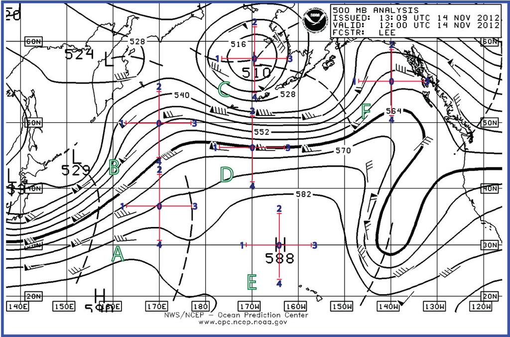
8 The equation that you developed states that the 500 mb relative geostrophic vorticity (hereafter called relative vorticity, remembering that the geostrophic vorticity is the real vorticity only at the level where the wind is actually geostrophic, nominally, at the 500 mb level) can be obtained if the analyst can obtain 500 mb heights at each of the five grid points. That s all you need to know about height/pressure gradients...just a map of heights. You will have to calculate f, the Coriolis parameter, which we already have learned is f = 2Ωsinφ (5) to obtain the quotient g/f. You can construct a spreadsheet to do this or you can use: To convert to absolute geostrophic vorticity (hereafter referred to as absolute vorticity) all you then have to do is to add the value of the Coriolis parameter to the result. Numerical schemes can do this directly from the upper air data gridded on the basis of information from the radiosonde sites. The 500 mb heights are interpolated to the grid points using various objective schemes. The analyst can perform an analogous procedure if he or she is presented with a map of 500 mb heights in the field. A careful contouring of the data can lead to adequate estimates for the 500 mb heights at the grid points. The contours are meticulously constructed making sure they are oriented correctly with respect to the wind field (wind flow parallel to the contours and contour spacing inversely proportional to the wind strength). Map Exercise 1. (60 points) For the 500 mb chart given, calculate the absolute geostrophic vorticity at the locations at the center of each of the six finite difference crosses plotted. Each cross has dimensions of d=5 deg latitude. Recall that each deg of latitude as length of 111 km. Work in teams, as discussed in class. First, compute the relative geostrophic vorticity at each central grid point. To do this you will need to determine the heights at each of the locations on the finite difference cross. You will have to compute the quantity in brackets in equation (3) above and then multiply by g/f. 8

9 Second, to convert relative vorticity to absolute vorticity you must add the value of f at that latitude Remember to keep your units consistent. Record right on the 500 mb chart under the center point of the grid. Map Exercise 2. (40 points) Once the values are obtained, compare your values to those you can infer from the attached 500 mb/absolute Vorticity analysis from the GFS. Remember, the GFS is calculating real absolute vorticity, not the absolute geostrophic vorticity. But it will be interesting for you to see how your results compare. Also, you ll learn something about typical relative and absolute vorticity values. The values I obtained were close but not exactly the same as the values evident on the GFS absolute vorticity chart for the day and time in question. I attribute the errors to two things (a) I may have used incorrect estimates of the heights in evaluating the Laplacian; (b) even if my height values are correct, the absolute vorticity of the geostrophic wind may not be the same as the absolute vorticity of the 500 mb height pattern (even though the two should be close); and, (c) it was difficult to interpolate the GFS absolute vorticity values in areas without color fill, so my estimates could be off. 9

10 Synthesis Question 1: Examination of Your Pattern (20 points) Mathematicians tell us that the Laplacian operation returns the inverse relative values of the field it operates on. For example, the Laplacian acting on a grid point at which the temperature is a maximum will return a negative number (a minimum). How is that illustrated by what you found in Map Exercise 1. The Laplacian of a local maximum field of values will return a minimum and vice versa. Thus, the Laplacian of the height field centered in a cyclone will return a relative vorticity maximum, and the Laplacian of the height field centered in an anticyclone will return a relative vorticity minimum. In the case of my values shown above, the largest value of positive relative vorticity was at location C, at which location a closed low in the height field was found. I also calculated a large negative relative vorticity at location E, at which location a closed anticyclone was found in the height field. Synthesis Question 2: Natural Coordinate Definition of Relative Vorticity (20 points) Explain why absolute vorticity contours seem to cut across height contours for sinusoidal patterns (say, at 500 mb) but seem to be parallel to contours for closed systems. Curvature vorticity for a given wind shear will be exactly the same for a concentric pattern of closed isobars, whether anticyclonic or cyclonic. Assuming that the height gradient is exactly the same, then relative vorticity contours will be parallel to the height contours, with the highest value at the innermost contour, in which the radius of curvature is very small. Even for patterns that span many degrees of latitude, the Coriolis parameter does not vary much. Hence, the pattern described here is even evident in the field of absolute vorticity contours. 10

11

12 12