ERTH 465 Fall Lab 8 Key. Absolute Geostrophic Vorticity. 200 points. 1. Answer questions with complete sentences on separate sheets.

Transcription

1 Name Date ERTH 465 Fall 2017 Lab 8 Key Absolute Geostrophic Vorticity 200 points. 1. Answer questions with complete sentences on separate sheets. 2. Show all work in mathematical problems. No credit given if only answer is provided.

2 A. Introduction Kinematically, relative vertical vorticity is z = v x - u y (1) where u and v are the horizontal wind components. In examining equation (1), you ll note that the terms to the right of the equals sign are merely spatial derivatives of wind components. You already found out in our previous work and discussions in this class that these kinds of derivatives can easily (but tediously) estimated by finite difference techniques If we apply equation (1) at the Level of Non-divergence, roughly the 500 mb level, then we know that the wind components themselves must be nearly geostrophic, and here are the two components. u g = g f z y v g = g f z x (2) By substitution of Equations (2) into (1), the relative and absolute vorticity of the geostrophic wind can be obtained directly from the height field without the analyst going through the intermediate step of specifying the gradients of the wind components. (You will derive the appropriate equation below). Since the level at which the real wind is most nearly geostrophic (nondivergent) is around the 500 mb level, the absolute geostrophic vorticity field is an accurate representation of the real vorticity field at that level. Thus, the vorticity patterns at 300 mb (or, at any level, for that matter) can be qualitatively diagnosed by the patterns of geostrophic vorticity patterns at the level of nondivergence (which, we assume, is near the 500 mb level). 2

3 In this lab you will learn how closely the actual 500 mb vorticity on a real 500 mb chart corresponds to the values you will get assuming that the wind is geostrophic at that level. You ll also be using the notational convention of collapsing and simplifying the second derivatives with respect to distance into the Laplacian. 3

4 B. Exercises Exercise 1: Substitute the geostrophic wind equations (in x,y,p) coordinates, as given in equation (2) above into equation (1) and expand. Assume that the Coriolis parameter is constant. (30 points) Simplify using Ñ h 2 = 2 x y 2 (3) z = v x - u y u g = - g z f y v g = g z f x z g = - g f æ æ z ö ç ç è x ø çç x ç è - (1) (2a) (2b) æ z ö ö ç è y ø (3) y ø z g = - g f Ñ2 z (4) where (2) is the horizontal Laplacian and provides a quantitative estimate of the shape of the field in question (in this case, the heights). The Laplacian of the height field is an estimate of the variation of the slope of the height field along the horizontal coordinate axes. 4

5 Note the finite difference grid below. The crosses below indicate grid points at which heights are recorded. The grid points are labeled (unconventionally) 0,1,2,3,4,A,B,C and D and are all located at distance of "s" and 2s = d, the grid distance from points 1, 2, 3, and 4 from the central grid point 0. The derivative expression (Z1 - Z0)/d can be evaluated at point A by the finite difference and at point C can be approximated by the expression (Z0 - Z3)/d. The derivative æ z ö è y ø æ z ö è y ø æ æ z ö ç è y ø ç y è ö ø can be obtained by subtracting the height gradient at C from that at A (both obtained above) and dividing by the distance between A and C, which is d. The result is the finite difference approximation for the term furthest to the right of the equals sign in the equation you developed in Question 1 above. Exercise 2. 5

6 Perform the same derivation for the first term to the right of the equals sign in the equation you developed in Question 1 above. Algebraically add the results in this section to obtain the full finite difference equivalent for the equation you developed in Question 1 above. (30 points) g f 2 z = g f [ (z 1+z 2 +z 3 +z 4 +z 0 ) ] d 2 The finite difference equation you developed above states that the relative vorticity is directly proportional to the shape of the height field as estimated for the variation in slope of the height surface along the two coordinate axes. g f 2 z = g f [ (z 1+z 2 +z 3 +z 4 +z 0 ) ] (4) d 2 where d is the grid distance (the distance between the origin and the adjacent numbered grid points. You are nearly ready to compute absolute geostrophic vorticity from the map of 500 mb data attached. However, to compute absolute vorticity one needs to know the value of the Coriolis parameter at the same range of latitudes as given above. The equation that you developed states that the 500 mb relative geostrophic vorticity (hereafter called relative vorticity, remembering that the geostrophic vorticity is the real vorticity only at the level where the wind is actually geostrophic, nominally, at the 500 mb level) can be obtained if the analyst can obtain 500 mb heights at each of the five grid points The equation for absolute geostrophic vorticity is as follows, with the substitutions from equation (4) made sequentially: η g = ζ g + f η g = g f 2 z + f (5) 6

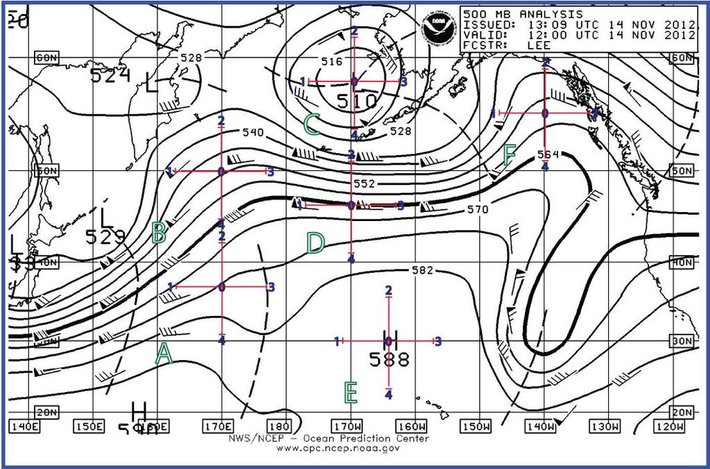
7 η g = g f [ (z 1+z 2 +z 3 +z 4 +z 0 ) ] + f d 2 That s all you need to know about height/pressure gradients...just a map of heights. You will have to calculate f, the Coriolis parameter, which we already have learned is f = 2Ωsinφ (6) to obtain the quotient g/f, since g is constant. You can construct a spreadsheet to compute the value of f at the gridpoints or you can use: To convert to absolute geostrophic vorticity (hereafter referred to as absolute vorticity) all you then have to do is to add the value of the Coriolis parameter to the result. Numerical schemes can do this directly from the upper air data gridded on the basis of information from the radiosonde sites. The 500 mb heights are interpolated to the grid points using various objective schemes. The analyst can perform an analogous procedure if he or she is presented with a map of 500 mb heights in the field. A careful contouring of the data can lead to adequate estimates for the 500 mb heights at the grid points. The contours are meticulously constructed making sure they are oriented correctly with respect to the wind field (wind flow parallel to the contours and contour spacing inversely proportional to the wind strength). Map Exercise 1. (60 points) For the 500 mb chart given, calculate the absolute geostrophic vorticity at the locations at the center of each of the six finite difference crosses plotted. Each cross has dimensions of d=5 deg latitude. Recall that each deg of latitude as length of 111 km. 7

8 Work in teams, as discussed in class. First, compute the relative geostrophic vorticity at each central grid point. To do this you will need to determine the heights at each of the locations on the finite difference cross. You will have to compute the quantity in brackets in equation (3) above and then multiply by g/f. Second, to convert relative vorticity to absolute vorticity you must add the value of f at that latitude Remember to keep your units consistent. Record right on the 500 mb chart under the center point of the grid. Map Exercise 2. (40 points) Once the values are obtained, compare your values to those you can infer from the attached 500 mb/absolute Vorticity analysis from the GFS. Remember, the GFS is calculating real absolute vorticity, not the absolute geostrophic vorticity. But it will be interesting for you to see how your 8

9 results compare. Also, you ll learn something about typical relative and absolute vorticity values. The values I obtained were close but not exactly the same as the values evident on the GFS absolute vorticity chart for the day and time in question. I attribute the errors to two things (a) I may have used incorrect estimates of the heights in evaluating the Laplacian; (b) even if my height values are correct, the absolute vorticity of the geostrophic wind may not be the same as the absolute vorticity of the 500 mb height pattern (even though the two should be close); and, (c) it was difficult to interpolate the GFS absolute vorticity values in areas without color fill, so my estimates could be off. Synthesis Question 1: Examination of Your Pattern (20 points) Mathematicians tell us that the Laplacian operation returns the inverse relative values of the field it operates on. For example, the Laplacian acting on a grid point at which the temperature is a maximum will return a negative number (a minimum). How is that illustrated by what you found in Map Exercise 1. The Laplacian of a local maximum field of values will return a minimum and vice versa. Thus, the Laplacian of the height field centered in a cyclone will return a relative vorticity maximum, and the Laplacian of the height field centered in an anticyclone will return a relative vorticity minimum. In the case of my values shown above, the largest value of positive relative vorticity was at location C, at which location a closed low in the height field was found. I also calculated a large negative relative vorticity at 9

10 location E, at which location a closed anticyclone was found in the height field. Synthesis Question 2: Natural Coordinate Definition of Relative Vorticity (20 points) Explain why absolute vorticity contours seem to cut across height contours for sinusoidal patterns (say, at 500 mb) but seem to be parallel to contours for closed systems. Curvature vorticity for a given wind shear will be exactly the same for a concentric pattern of closed isobars, whether anticyclonic or cyclonic. Assuming that the height gradient is exactly the same, then relative vorticity contours will be parallel to the height contours, with the highest value at the innermost contour, in which the radius of curvature is very small. Even for patterns that span many degrees of latitude, the Coriolis parameter does not vary much. Hence, the pattern described here is even evident in the field of absolute vorticity contours. 10

11

12

13 13