An Introduction to Linear Programming

Size: px

Start display at page:

Download "An Introduction to Linear Programming"

Lee Shaw
5 years ago
Views:

1 An Introduction to Linear Programming Linear Programming Problem Problem Formulation A Maximization Problem Graphical Solution Procedure Extreme Points and the Optimal Solution Computer Solutions A Minimization Problem Special Cases Linear Programming Applications Linear Programming (LP) Problem The maximization or minimization of some quantity is the objective in all linear programming problems. All LP problems have constraints that limit the degree to which the objective can be pursued. A feasible solution satisfies all the problem's constraints. An optimal solution is a feasible solution that results in the largest possible objective function value when maximizing (or smallest when minimizing). A graphical solution method can be used to solve a linear program with two variables. 1

2 Linear Programming (LP) Problem If both the objective function and the constraints are linear, the problem is referred to as a linear programming problem. Linear functions are functions in which each variable appears in a separate term raised to the first power and is multiplied by a constant (which could be 0). Linear constraints are linear functions that are restricted to be "less than or equal to", "equal to", or "greater than or equal to" a constant. Problem Formulation Problem formulation or modeling is the process of translating a verbal statement of a problem into a mathematical statement. 2

3 Guidelines for Model Formulation Understand the problem thoroughly. Describe the objective. Describe each constraint. Define the decision variables. Write the objective in terms of the decision variables. Write the constraints in terms of the decision variables. Example 1: A Maximization Problem LP Formulation Max 5x 1 + 7x 2 s.t. x 1 < 6 2x 1 + 3x 2 <19 x 1 + x 2 < 8 x 1, x 2 >0 3

4 Example 1: Graphical Solution Constraint #1 Graphed x x 1 < (6, 0) x 1 Example 1: Graphical Solution Constraint #2 Graphed x (0, 6 1/3) x 1 + 3x 2 < (9 1/2, 0) x 1 4

5 Example 1: Graphical Solution Constraint #3 Graphed x 2 (0, 8) x 1 + x 2 < (8, 0) x 1 Example 1: Graphical Solution Combined-Constraint Graph x 2 8 x 1 + x 2 <8 7 6 x 1 < x 1 + 3x 2 < x 1 5

6 Example 1: Graphical Solution Feasible Solution Region x Feasible Region x 1 Example 1: Graphical Solution Objective Function Line x (0, 5) Objective Function 5x 1 + 7x 2 = (7, 0) x 1 6

7 Optimal Solution Example 1: Graphical Solution x Objective Function 5x 1 + 7x 2 = 46 Optimal Solution (x 1 = 5, x 2 = 3) x 1 Summary of the Graphical Solution Procedure for Maximization Problems Prepare a graph of the feasible solutions for each of the constraints. Determine the feasible region that satisfies all the constraints simultaneously.. Draw an objective function line. Move parallel objective function lines toward larger objective function values without entirely leaving the feasible region. Any feasible solution on the objective function line with the largest value is an optimal solution. 7

8 Slack and Surplus Variables A linear program in which all the variables are nonnegative and all the constraints are equalities is said to be in standard form. Standard form is attained by adding slack variables to "less than or equal to" constraints, and by subtracting surplus variables from "greater than or equal to" constraints. Slack and surplus variables represent the difference between the left and right sides of the constraints. Slack and surplus variables have objective function coefficients equal to 0. Standard Form Example 1 Max 5x 1 + 7x 2 + 0s 1 + 0s 2 + 0s 3 s.t. x 1 + s 1 = 6 2x 1 + 3x 2 + s 2 = 19 x 1 + x 2 + s 3 = 8 x 1, x 2, s 1, s 2, s 3 >0 8

9 Extreme Points and the Optimal Solution The corners or vertices of the feasible region are referred to as the extreme points. An optimal solution to an LP problem can be found at an extreme point of the feasible region. When looking for the optimal solution, you do not have to evaluate all feasible solution points. You have to consider only the extreme points of the feasible region. Example 1: Graphical Solution The Five Extreme Points x Feasible 3 Region x 1 9

10 Computer Solutions Computer programs designed to solve LP problems are now widely available. Most large LP problems can be solved with just a few minutes of computer time. Small LP problems usually require only a few seconds. Linear programming solvers are now part of many spreadsheet packages, such as Microsoft Excel. Interpretation of Computer Output In this chapter we will discuss the following output: objective function value values of the decision variables reduced costs slack/surplus In Chapter 3 we will discuss how an optimal solution is affected by a change in: a coefficient of the objective function the right-hand side value of a constraint 10

11 Example 1: Spreadsheet Solution Partial Spreadsheet Showing Problem Data Example 1: Spreadsheet Solution Partial Spreadsheet Showing Solution 11

12 Example 1: Spreadsheet Solution Interpretation of Computer Output We see from the previous slide that: Objective Function Value = 46 Decision Variable #1 (x 1 ) = 5 Decision Variable #2 (x 2 ) = 3 Slack in Constraint #1 = 1 (= 6-5) Slack in Constraint #2 = 0 (= 19-19) Slack in Constraint #3 = 0 (= 8-8) Reduced Cost The reduced cost for a decision variable whose value is 0 in the optimal solution is the amount the variable's objective function coefficient would have to improve (increase for maximization problems, decrease for minimization problems) before this variable could assume a positive value. The reduced cost for a decision variable with a positive value is 0. 12

13 Reduced Costs Example 1: Spreadsheet Solution Example 2: A Minimization Problem LP Formulation Min 5x 1 + 2x 2 s.t. 2x 1 + 5x 2 >10 4x 1 - x 2 >12 x 1 + x 2 > 4 x 1, x 2 >0 13

14 Example 2: Graphical Solution Graph the Constraints Constraint 1: When x 1 = 0, then x 2 = 2; when x 2 = 0, then x 1 = 5. Connect (5,0) and (0,2). The ">" side is above this line. Constraint 2: When x 2 = 0, then x 1 = 3. But setting x 1 to 0 will yield x 2 = -12, which is not on the graph. Thus, to get a second point on this line, set x 1 to any number larger than 3 and solve for x 2 : when x 1 = 5, then x 2 = 8. Connect (3,0) and (5,8). The ">" side is to the right. Constraint 3: When x 1 = 0, then x 2 = 4; when x 2 = 0, then x 1 = 4. Connect (4,0) and (0,4). The ">" side is above this line. Example 2: Graphical Solution Constraints Graphed x Feasible Region 4x 1 - x 2 >12 x 1 + x 2 >4 2x 1 + 5x 2 > x 1 14

15 Example 2: Graphical Solution Graph the Objective Function Set the objective function equal to an arbitrary constant (say 20) and graph it. For 5x 1 + 2x 2 = 20, when x 1 = 0, then x 2 = 10; when x 2 = 0, then x 1 = 4. Connect (4,0) and (0,10). Move the Objective Function Line Toward Optimality Move it in the direction which lowers its value (down), since we are minimizing, until it touches the last point of the feasible region, determined by the last two constraints. Example 2: Graphical Solution Objective Function Graphed x 2 Min z = 5x 1 + 2x 2 x x 1 - x 2 >12 x 1 + x 2 >4 2x 1 + 5x 2 > x 1 15

16 Example 2: Graphical Solution Solve for the Extreme Point at the Intersection of the Two Binding Constraints 4x 1 - x 2 = 12 x 1 + x 2 = 4 Adding these two equations gives: 5x 1 = 16 or x 1 = 16/5. Substituting this into x 1 + x 2 = 4 gives: x 2 = 4/5 Example 2: Graphical Solution Solve for the Optimal Value of the Objective Function Solve for z = 5x 1 + 2x 2 = 5(16/5) + 2(4/5) = 88/5. Thus the optimal solution is x 1 = 16/5; x 2 = 4/5; z = 88/5 16

Example 2: Graphical Solution Optimal Solution x 2 Min z = 5x 1 + 2x 2 x 2 5 4 3 2 1 4x 1 - x 2 >12 x 1 + x 2 >4 2x 1 + 5x 2

17 Example 2: Graphical Solution Optimal Solution x 2 Min z = 5x 1 + 2x 2 x x 1 - x 2 >12 x 1 + x 2 >4 2x 1 + 5x 2 >10 Optimal: x 1 = 16/5 x 2 = 4/ x 1 Example 2: Spreadsheet Solution Partial Spreadsheet Showing Problem Data 17

18 Example 2: Spreadsheet Solution Partial Spreadsheet Showing Formulas Example 2: Spreadsheet Solution Partial Spreadsheet Showing Solution 18

19 Feasible Region The feasible region for a two-variable linear programming problem can be nonexistent, a single point, a line, a polygon, or an unbounded area. Any linear program falls in one of three categories: is infeasible has a unique optimal solution or alternate optimal solutions has an objective function that can be increased without bound A feasible region may be unbounded and yet there may be optimal solutions. This is common in minimization problems and is possible in maximization problems. Special Cases Alternative Optimal Solutions In the graphical method, if the objective function line is parallel to a boundary constraint in the direction of optimization, there are alternate optimal solutions, with all points on this line segment being optimal. Infeasibility A linear program which is overconstrained so that no point satisfies all the constraints is said to be infeasible. Unboundedness (See example on upcoming slide.) 19

20 Example: Infeasible Problem Solve graphically for the optimal solution: Max 2x 1 + 6x 2 s.t. 4x 1 + 3x 2 <12 2x 1 + x 2 > 8 x 1, x 2 >0 Example: Infeasible Problem There are no points that satisfy both constraints, hence this problem has no feasible region, and no optimal solution. x 2 8 2x 1 + x 2 >8 4 4x 1 + 3x 2 < x 1 20

21 Example: Unbounded Problem Solve graphically for the optimal solution: Max 3x 1 + 4x 2 s.t. x 1 + x 2 >5 3x 1 + x 2 >8 x 1, x 2 >0 Example: Unbounded Problem The feasible region is unbounded and the objective function line can be moved parallel to itself without bound so that z can be increased infinitely. x 2 3x 1 + x 2 > Max 3x 1 + 4x 2 x 1 + x 2 > x 1 21

22 Linear Programming Applications Blending Problem Portfolio Planning Problem Product Mix Problem Transportation Problem Data Envelopment Analysis Blending Problem Frederick's Feed Company receives four raw grains from which it blends its dry pet food. The pet food advertises that each 8-ounce can meets the minimum daily requirements for vitamin C, protein and iron. The cost of each raw grain as well as the vitamin C, protein, and iron units per pound of each grain are summarized on the next slide. Frederick's is interested in producing the 8-ounce mixture at minimum cost while meeting the minimum daily requirements of 6 units of vitamin C, 5 units of protein, and 5 units of iron. 22

23 Blending Problem Vitamin C Protein Iron Grain Units/lb Units/lb Units/lb Cost/lb Blending Problem Define the decision variables x j = the pounds of grain j (j = 1,2,3,4) used in the 8-ounce mixture Define the objective function Minimize the total cost for an 8-ounce mixture: MIN.75x x x x 4 23

24 Blending Problem Define the constraints Total weight of the mix is 8-ounces (.5 pounds): (1) x 1 + x 2 + x 3 + x 4 =.5 Total amount of Vitamin C in the mix is at least 6 units: (2) 9x x 2 + 8x x 4 > 6 Total amount of protein in the mix is at least 5 units: (3) 12x x x 3 + 8x 4 > 5 Total amount of iron in the mix is at least 5 units: (4) 14x x 3 + 7x 4 > 5 Nonnegativity of variables: x j > 0 for all j Blending Problem The Management Scientist Output OBJECTIVE FUNCTION VALUE = VARIABLE VALUE REDUCED COSTS X X X X Thus, the optimal blend is about.10 lb. of grain 1,.21 lb. of grain 2,.09 lb. of grain 3, and.10 lb. of grain 4. The mixture costs Frederick s 40.6 cents. 24

25 Portfolio Planning Problem Winslow Savings has $20 million available for investment. It wishes to invest over the next four months in such a way that it will maximize the total interest earned over the four month period as well as have at least $10 million available at the start of the fifth month for a high rise building venture in which it will be participating. Portfolio Planning Problem For the time being, Winslow wishes to invest only in 2-month government bonds (earning 2% over the 2- month period) and 3-month construction loans (earning 6% over the 3-month period). Each of these is available each month for investment. Funds not invested in these two investments are liquid and earn 3/4 of 1% per month when invested locally. 25

26 Portfolio Planning Problem Formulate a linear program that will help Winslow Savings determine how to invest over the next four months if at no time does it wish to have more than $8 million in either government bonds or construction loans. Portfolio Planning Problem Define the decision variables g j c j = amount of new investment in government bonds in month j = amount of new investment in construction loans in month j l j = amount invested locally in month j, where j = 1,2,3,4 26

27 Portfolio Planning Problem Define the objective function Maximize total interest earned over the 4-month period. MAX (interest rate on investment)(amount invested) MAX.02g g g g c c c c l l l l 4 Define the constraints Portfolio Planning Problem Month 1's total investment limited to $20 million: (1) g 1 + c 1 + l 1 = 20,000,000 Month 2's total investment limited to principle and interest invested locally in Month 1: (2) g 2 + c 2 + l 2 = l 1 or g 2 + c l 1 + l 2 = 0 27

28 Portfolio Planning Problem Define the constraints (continued) Month 3's total investment amount limited to principle and interest invested in government bonds in Month 1 and locally invested in Month 2: (3) g 3 + c 3 + l 3 = 1.02g l 2 or g 1 + g 3 + c l 2 + l 3 = 0 Portfolio Planning Problem Define the constraints (continued) Month 4's total investment limited to principle and interest invested in construction loans in Month 1, goverment bonds in Month 2, and locally invested in Month 3: (4) g 4 + c 4 + l 4 = 1.06c g l 3 or g 2 + g c 1 + c l 3 + l 4 = 0 $10 million must be available at start of Month 5: (5) 1.06c g l 4 > 10,000,000 28

29 Portfolio Planning Problem Define the constraints (continued) No more than $8 million in government bonds at any time: (6) g 1 < 8,000,000 (7) g 1 + g 2 < 8,000,000 (8) g 2 + g 3 < 8,000,000 (9) g 3 + g 4 < 8,000,000 Portfolio Planning Problem Define the constraints (continued) No more than $8 million in construction loans at any time: (10) c 1 < 8,000,000 (11) c 1 + c 2 < 8,000,000 (12) c 1 + c 2 + c 3 < 8,000,000 (13) c 2 + c 3 + c 4 < 8,000,000 Nonnegativity: g j, c j, l j > 0 for j = 1,2,3,4 29

30 Problem: Floataway Tours Floataway Tours has $420,000 that may be used to purchase new rental boats for hire during the summer. The boats can be purchased from two different manufacturers. Floataway Tours would like to purchase at least 50 boats and would like to purchase the same number from Sleekboat as from Racer to maintain goodwill. At the same time, Floataway Tours wishes to have a total seating capacity of at least 200. Pertinent data concerning the boats are summarized on the next slide. Formulate this problem as a linear program. Problem: Floataway Tours Data Maximum Expected Boat Builder Cost Seating Daily Profit Speedhawk Sleekboat $ $ 70 Silverbird Sleekboat $ $ 80 Catman Racer $ $ 50 Classy Racer $ $110 30

31 Problem: Floataway Tours Define the decision variables x 1 = number of Speedhawks ordered x 2 = number of Silverbirds ordered x 3 = number of Catmans ordered x 4 = number of Classys ordered Define the objective function Maximize total expected daily profit: Max: (Expected daily profit per unit) x (Number of units) Max: 70x x x x 4 Problem: Floataway Tours Define the constraints (1) Spend no more than $420,000: 6000x x x x 4 < 420,000 (2) Purchase at least 50 boats: x 1 + x 2 + x 3 + x 4 >50 (3) Number of boats from Sleekboat equals number of boats from Racer: x 1 + x 2 = x 3 + x 4 or x 1 + x 2 - x 3 - x 4 = 0 31

32 Problem: Floataway Tours Define the constraints (continued) (4) Capacity at least 200: 3x 1 + 5x 2 + 2x 3 + 6x 4 > 200 Nonnegativity of variables: x j > 0, for j = 1,2,3,4 Complete Formulation Problem: Floataway Tours Max 70x x x x 4 s.t. 6000x x x x 4 < 420,000 x 1 + x 2 + x 3 + x 4 >50 x 1 + x 2 - x 3 - x 4 = 0 3x 1 + 5x 2 + 2x 3 + 6x 4 > 200 x 1, x 2, x 3, x 4 >0 32

33 Problem: Floataway Tours Partial Spreadsheet Showing Problem Data Problem: Floataway Tours Partial Spreadsheet Showing Solution 33

34 Problem: Floataway Tours The Management Science Output OBJECTIVE FUNCTION VALUE = Variable Value Reduced Cost x x x x Constraint Slack/Surplus Dual Price Problem: Floataway Tours Solution Summary Purchase 28 Speedhawks from Sleekboat. Purchase 28 Classy s from Racer. Total expected daily profit is $5, The minimum number of boats was exceeded by 6 (surplus for constraint #2). The minimum seating capacity was exceeded by 52 (surplus for constraint #4). 34

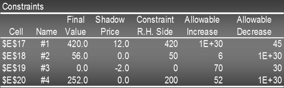
35 Sensitivity Report Problem: Floataway Tours Sensitivity Report Problem: Floataway Tours 35

36 Problem: U.S. Navy The Navy has 9,000 pounds of material in Albany, Georgia which it wishes to ship to three installations: San Diego, Norfolk, and Pensacola. They require 4,000, 2,500, and 2,500 pounds, respectively. Government regulations require equal distribution of shipping among the three carriers. The shipping costs per pound for truck, railroad, and airplane transit are shown on the next slide. Formulate and solve a linear program to determine the shipping arrangements (mode, destination, and quantity) that will minimize the total shipping cost. Problem: U.S. Navy Data Mode Destination San Diego Norfolk Pensacola Truck $12 $ 6 $ 5 Railroad Airplane

37 Problem: U.S. Navy Define the Decision Variables We want to determine the pounds of material, x ij, to be shipped by mode i to destination j. The following table summarizes the decision variables: San Diego Norfolk Pensacola Truck x 11 x 12 x 13 Railroad x 21 x 22 x 23 Airplane x 31 x 32 x 33 Problem: U.S. Navy Define the Objective Function Minimize the total shipping cost. Min: (shipping cost per pound for each mode per destination pairing) x (number of pounds shipped by mode per destination pairing). Min: 12x x x x x x x x x 33 37

38 Problem: U.S. Navy Define the Constraints Equal use of transportation modes: (1) x 11 + x 12 + x 13 = 3000 (2) x 21 + x 22 + x 23 = 3000 (3) x 31 + x 32 + x 33 = 3000 Destination material requirements: (4) x 11 + x 21 + x 31 = 4000 (5) x 12 + x 22 + x 32 = 2500 (6) x 13 + x 23 + x 33 = 2500 Nonnegativity of variables: x ij > 0, i = 1,2,3 and j = 1,2,3 Problem: U.S. Navy Partial Spreadsheet Showing Problem Data 38

Problem: U.S. Navy Partial Spreadsheet Showing Solution Problem: U.S. Navy The Management Scientist Output OBJECTIVE FUNCTION VALUE = 142000.

39 Problem: U.S. Navy Partial Spreadsheet Showing Solution Problem: U.S. Navy The Management Scientist Output OBJECTIVE FUNCTION VALUE = Variable Value Reduced Cost x x x x x x x x x

40 Problem: U.S. Navy Solution Summary San Diego will receive 1000 lbs. by truck and 3000 lbs. by airplane. Norfolk will receive 2000 lbs. by truck and 500 lbs. by railroad. Pensacola will receive 2500 lbs. by railroad. The total shipping cost will be $142,000. Data Envelopment Analysis Data envelopment analysis (DEA) is an LP application used to determine the relative operating efficiency of units with the same goals and objectives. DEA creates a fictitious composite unit made up of an optimal weighted average (W 1, W 2, ) of existing units. An individual unit, k, can be compared by determining E, the fraction of unit k s input resources required by the optimal composite unit. If E < 1, unit k is less efficient than the composite unit and be deemed relatively inefficient. If E = 1, there is no evidence that unit k is inefficient, but one cannot conclude that k is absolutely efficient. 40

41 The DEA Model MIN E s.t. Data Envelopment Analysis Weighted outputs > Unit k s output (for each measured output) Weighted inputs < E [Unit k s input] (for each measured input) Sum of weights = 1 E, weights > 0 DEA Example: Roosevelt High The Langley County School District is trying to determine the relative efficiency of its three high schools. In particular, it wants to evaluate Roosevelt High School. The district is evaluating performances on SAT scores, the number of seniors finishing high school, and the number of students who enter college as a function of the number of teachers teaching senior classes, the prorated budget for senior instruction, and the number of students in the senior class. 41

42 DEA Example: Roosevelt High Input Roosevelt Lincoln Washington Senior Faculty Budget ($100,000's) Senior Enrollments DEA Example: Roosevelt High Output Roosevelt Lincoln Washington Average SAT Score High School Graduates College Admissions

43 Decision Variables DEA Example: Roosevelt High E = Fraction of Roosevelt's input resources required by the composite high school w 1 = Weight applied to Roosevelt's input/output resources by the composite high school w 2 = Weight applied to Lincoln s input/output resources by the composite high school w 3 = Weight applied to Washington's input/output resources by the composite high school Objective Function DEA Example: Roosevelt High Minimize the fraction of Roosevelt High School's input resources required by the composite high school: MIN E 43

44 Constraints DEA Example: Roosevelt High Sum of the Weights is 1: (1) w 1 + w 2 + w 3 = 1 Output Constraints: Since w 1 = 1 is possible, each output of the composite school must be at least as great as that of Roosevelt: (2) 800w w w 3 > 800 (SAT Scores) (3) 450w w w 3 > 450 (Graduates) (4) 140w w w 3 > 140 (College Admissions) Constraints DEA Example: Roosevelt High Input Constraints: The input resources available to the composite school is a fractional multiple, E, of the resources available to Roosevelt. Since the composite high school cannot use more input than that available to it, the input constraints are: (5) 37w w w 3 < 37E (Faculty) (6) 6.4w w w 3 < 6.4E (Budget) (7) 850w w w 3 < 850E (Seniors) Nonnegativity of variables: E, w 1, w 2, w 3 >0 44

45 DEA Example: Roosevelt High Management Scientist Output OBJECTIVE FUNCTION VALUE = VARIABLE VALUE REDUCED COSTS E W W W DEA Example: Roosevelt High Management Scientist Output CONSTRAINT SLACK/SURPLUS DUAL PRICES

46 DEA Example: Roosevelt High Conclusion The output shows that the composite school is made up of equal weights of Lincoln and Washington. Roosevelt is 76.5% efficient compared to this composite school when measured by college admissions (because of the 0 slack on this constraint (#4)). It is less than 76.5% efficient when using measures of SAT scores and high school graduates (there is positive slack in constraints 2 and 3.) 46

Graphical and Computer Methods

Chapter 7 Linear Programming Models: Graphical and Computer Methods Quantitative Analysis for Management, Tenth Edition, by Render, Stair, and Hanna 2008 Prentice-Hall, Inc. Introduction Many management