Operations depend on pixel s Coordinates. Context free. Independent of pixel values. I(x,y) I (x,y )

Transcription

1

2 Geometric Transformation Operations depend on piel s Coordinates. Contet free. Independent of piel values. f f (, ) = ' (, ) = ' I(, ) = I' ( f (, ), f ( ) ), (,) (, ) I(,) I (, )

3 Eample: Translation = = f f (, ) = + 3 (, ) = ( + 3, ) I(, ) I ' = (,) (, ) I(,) I (, )

4 Forward Mapping Forward mapping: f f (, ) = (, ) = Source Target Forward Mapping Problems with forward mapping due to sampling: Holes (some target piels are not populated) Overlaps (some target piels assigned few colors)

5 Forward Mapping = f =, 2 ( ) Source = f =, Target ( ) = =2 = =2 =3 =4 = f =,. 7 ( ) Source? = f =, Target ( ) = =2 = =2

6 Inverse Mapping Inverse mapping: f f (, ) = (, ) = Source Target Inverse Mapping Each target piel assigned a single color. Color Interpolation is reuired.

7 Eample: Scaling along X Forward mapping: Source (,) = 2 ; = Target (,) Inverse mapping: = / 2 ; = Source Target

8 Interpolation What happens when a mapping function calculates a fractional piel location? Interpolation: generates a new piel b analzing the surrounding piels.

9 Interpolation Good interpolation techniues attempt to find an optimal balance between three undesirable artifacts: aliasing, blurring, and edge halos. 4 scaling aliasing blurring halos 9

10 Nearest Neighbor Interpolation The assign value is taken from the piel closest to the generated location: I Advantage: Fast Disadvantage: (, ) = I round f (, ) Jagged results Aliasing near edges ( { } {, round f (, ) })

11 Original Image Nearest N. Interpolation

12 Original Image Nearest N. Interpolation

13 Bilinear Interpolation The assign value is a weighted sum of the four nearest piels. Each weight is proportional to the distance from each eisting piel.

14 Linear Interpolation v e v w v w e e w w = v v e v v w w Isolating v in the above euation: v ( α) w = αv e + v where α = e w w

15 Bilinear Interpolation NW V N NE SW S SE S N V = SE + SW = NE + NW = N + S ( ) ( ) ( )

16 Bilinear Interpolation NW V N NE SW S SE The bilinear interpolation is the best fit low-degree polnomial of the form: v(, ) The piel s boundaries are C continuous (continuous values across boundaries). = i, j= a ij i j

17 Bilinear eample 5 z=5 z=7 v 5 z=2 z=

18 Nearest N. Interpolation Bilinear Interpolation

19 Nearest N. Interpolation Bilinear Interpolation

20 Bicubic Interpolation The assign value is a weighted sum of the 44 nearest piels: v(, ) = 3 i, j= a ij i j

21 How can we find the right coefficients? Denote the piel values V p {p,=..3} The unknown coefficients are a ij {i,j=..3} v p 3 = i, j= a ij i j for p, = {.. 3},, [ 2, ] We have a linear sstem of 6 euations with 6 coefficients. s The piel s boundaries are C continuous (continuous derivatives across boundaries). t 2

22 N.N Bilinear Bicubic

23 N.N

24 Bilinear

25 Bicubic

26 Appling the Transformation T = % 22 transformation matri [r,c] = size(img) % create arra of destination, coordinates [X,Y]=meshgrid(:c,:r); % calculate source coordinates sourcecoor = inv(t) * [X(:) Y(:) ] ; % calculate nearest neighbor interpolation Xs = round(sourcecoor(,:)); Ys = round(sourcecoor(2,:)); ind=find(xs< Xs>r); %out of range piels Xs(ind)=; Ys(ind)=; ind=find(ys< Ys>c); %out of range piels Xs(ind)=; Ys(ind)=; % calculate new image newimage = img((xs-).*r+ys); newimage(ind)=; newimage(ind)=; newimage = reshape(newimage,r,c);

27 Tpes of linear 2D transformations Rigid (Euclidean) transformation: Translation + Rotation (distance preserving). Similarit transformation: Translation + Rotation + Uniform Scale (angle preserving). Affine transformation: Translation + Rotation + Scale + Shear (parallelism preserving). Projective transformation Cross-ratio preserving All above transformations are groups where Rigid Similarit Affine Projective

28 Tpes of linear 2D transformations All above transformations are groups where Rigid Similarit Affine Projective

29 Matri Notation Ever location (,) is treated as a column vector: Coordinate transformation is obtained b multipling with a 22 matri? a c b d = a c + + b d

30 Matri Notation - Scale Scale(a,b): (,) (a,b) a b a = b If a or b are negative, we get reflection. Inverse: S - (a,b)=s(/a,/b) a ' ' b =

31 Matri Notation - Shear Shear(a,b): (,) (+a,+b) b a = + + a b a=.5, b=

32 Matri Notation - Rotation Rotate(θ): (,) (cosθ+sinθ, -sinθ + cosθ) cosθ sinθ cosθ + sinθ = sinθ cosθ sinθ + cosθ Inverse: R - (θ)=r T (θ)=r(-θ)

33 Matri Notation - Translation Translation(a,b): + + a b Cannot represent translation using 22 matrices. Inverse: a b

34 Homogeneous Coordinates Homogeneous Coordinates is a mapping from R n to R n+ : (, ) ( X, Y, W) ( t, t, t) Note: (t,t,t) all correspond to the same nonhomogeneous point (,). E.g. (2,3,) (6,9,3) (4,6,2). Inverse mapping: X W Y W ( X, Y, W), = (, )

35 Homogeneous Coordinates (t,t,t) (,) =(,,)

36 Some 2D Transformations Some 2D Transformations Translation : Affine transformation: Projective transformation: + + = = t t t t W Y X = t d c t b a W Y X = f e t d c t b a W Y X Affine

37 Hierarch of Linear 2D Transformations

38 Global Transformations Image Rectification

39 Global Transformations Global Warping = A

40 Global Transformations Global Warping Global Transformations Global Warping points p i points i match = p p p p p p A Y

41 Global Transformations Global Warping Global Transformations Global Warping points p i points i match = A p p p p p p Y Inverse Mapping:

42 Global Transformations Global Warping Solve for A - in terms of the least mean suare. i.e. find A - which minimizes: i pi A i 2

43 Global Transformations Global Warping Global Transformations Global Warping solution: ( ) ) ( = T XX T X X pinv = Y pinv p p p p p p A

44 Global Transformations Global Warping Global Transformations Global Warping Alternative representation: = f e d c b a = = f d c e b a A Rearrange:

45 Global Transformations Global Warping Global Transformations Global Warping = f e d cb a p p

46 Global Transformations Global Warping Global Transformations Global Warping = f e d cb a p p p p p p

47 Global Transformations Global Warping Global Transformations Global Warping = p p p p p p pinv f e d c b a ' ( ) T T Q Q Q Q pinv ) '( = solution:

48 Global Transformations Global Warping Global Transformations Global Warping What about Projective Transformations? = h g f d c e b a Homogeneit must be preserved! ' ; ' = = h g f d c h g e b a

49 Global Transformations Global Warping Global Transformations Global Warping What about Projective Transformations? ' ; ' = = h g f d c h g e b a ( ) = h g f e d c b a ' ' And similarl for

50 Global Transformations Image Rectification So who ARE we?

51 Local Transformations Image Warping Demo ale

52 Local Transformations Image Warping Area of influence Area of influence p s p s p d p d p s = source point p d = destination point

53 Local Transformations Image Warping Area of influence p s p s = source point p d = destination point p d destination p d p s p s source p d

54 Image Morphing (Image Metamorphosis) Demo bw

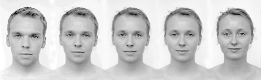
55 Cross Dissolve (piel operations) Source Image Destination Image t cross dissolve I ( t) = ( t) t [,] S + t T warp + dissolve

56 Warping + Cross Dissolve Warp source image towards intermediate image. Warp destination image towards intermediate image. Cross-dissolve the two images b taking the weighted average at each piel. source time Cross-dissolve destination warping images

57 warp Cross-dissolve Cross-dissolve warp

58 Image Metamorphosis Let S,T be the source and the target images Let G(p) be the transformation from S towards T, where G()=I (the identit) Let t [,] the time step to be snthesized Algorithm:. Warp S towards T: 2. Warp T toward S: 3. Cross dissolve: S T ( t) = G( t p){ S} I ( ) (( ) ) t = G t p { T} ( t) = ( t) S( t) + t T( t)

59 t sourse S(t)=G(t p){s} I(t)=(-t) S(t)+t (T(t)) target T(t)=G((-t) p) - {T}

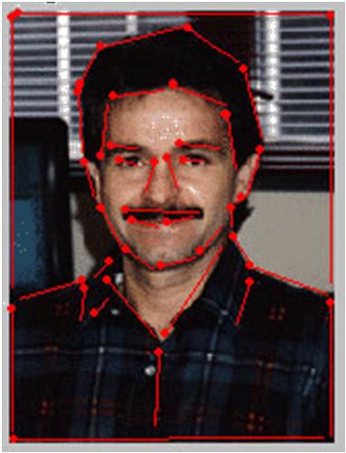
60 Feature Based Morphing Morph one shape into another shape Use local features to define the geometric warping

61 Q Q P P

62 Q Q P P

63 Q Q P P

64 Q Q P P

65 Q Q P P

66 Q Q P P

67 One Segment Warping Q β u v R α P Source Image Dest Image α [,] is the relative position along the segment (P,Q ). β is the actual perpendicular distance to the segment. (u,v ) is the local coordinates of the segment (P,Q ): u is a unit vector parallel to Q -P Q v is the unit vector perpendicular to Q -P ( Q P ) β α u v u u = Q P v = u = u R P

68 Q β R u v α P The point R is mapped into (α,β) : ( R P ) u α = ; β = Q P ( R P ) v where R' = P' + α Q' P' u' + βv'

69 Q u β v R α P Source Image Q u v β α Dest Image R P Inverse Mapping: R( α, β ) = P+ α Q P u+ βv where (u,v) is the local coordinates of the segment (P,Q): u ( Q P) = u Q P v= u= u

70 Multiple Segment Warping Q 2 Q Q 2 Q R β R 2 β 2 R β β 2 P P 2 P P 2 In multiple segment warping the point R is influenced b multiple segments. The influence strength of each segments is proportional to: Segment length The distance from the point R

71 The influence of each segments is: p Qi P i W i = a+β i The value p [,] controls the influence of the line length. The value a is a small number avoiding division b zero. The value b determines how the relative weight diminish as the β increases b The final mapping is: R = k k W R k W k k

72 Eample: Eample images from: For more details see: Thaddeus Beier & Shawn Neel / Feature-Based Image Metamorphosis Siggraph '92

73 Another Eample: 73

74 Mesh Warping From:

75 2-Pass Mesh Warping Algorithm The first pass warps the rows of the image: For each column of the mesh determine the -coordinates at which the mesh column crosses each image row.

76 2-Pass Mesh Warping Algorithm Then, each row of the image is warped individuall b linearl interpolating each segment between the -coordinates defined b the source mesh to the size of the corresponding segment defined b the -coordinates of the destination Mesh. The second pass performs the eact same procedure on the columns of the image b interpolating the -coordinates of the meshes.

77 VidMorph

78 Fun Morph