Contents. Signals as functions (1D, 2D)

Size: px

Start display at page:

Download "Contents. Signals as functions (1D, 2D)"

Silas James
6 years ago
Views:

1 Fourier Transform

The idea A signal can be interpreted as en electromagnetic wave. This consists of lights of different color, or frequency, that can be split apart usign an optic prism.

2 The idea A signal can be interpreted as en electromagnetic wave. This consists of lights of different color, or frequency, that can be split apart usign an optic prism. Each component is a monochromatic light with sinusoidal shape. Following this analogy, each signal can be decomposed into its sinusoidal components which represent its colors. Of course these components in general do not correspond to visible monochromatic light. However, they give an idea of how fast are the changes of the signal. 2

3 Contents Signals as functions (D, 2D) Tools Continuous Time Fourier Transform (CTFT) Discrete Time Fourier Transform (DTFT) Discrete Fourier Transform (DFT) Discrete Cosine Transform (DCT) Sampling theorem 3

4 Fourier Transform Different formulations for the different classes of signals Summary table: Fourier transforms with various combinations of continuous/ discrete time and frequency variables. Notations: CTFT: continuous time FT: t is real and f real (f=ω) (CT, CF) DTFT: Discrete Time FT: t is discrete (t=n), f is real (f=ω) (DT, CF) CTFS: CT Fourier Series (summation synthesis): t is real AND the function is periodic, f is discrete (f=k), (CT, DF) DTFS: DT Fourier Series (summation synthesis): t=n AND the function is periodic, f discrete (f=k), (DT, DF) P: periodical signals T: sampling period ω s : sampling frequency (ω s =2π/T) For DTFT: T= ω s =2π This is a hint for those who are interested in a more exhaustive theoretical approach 4

5 Images as functions Gray scale images: 2D functions Domain of the functions: set of (x,y) values for which f(x,y) is defined : 2D lattice [i,j] defining the pixel locations Set of values taken by the function : gray levels Digital images can be seen as functions defined over a discrete domain {i,j: 0<i<I, 0<j<J} I,J: number of rows (columns) of the matrix corresponding to the image f=f[i,j]: gray level in position [i,j] 5

6 Mathematical Background: Complex Numbers A complex number x is of the form: a: real part, b: imaginary part Addition Multiplication 6

7 Mathematical Background: Complex Numbers (cont d) Magnitude-Phase (i.e.,vector) representation Magnitude: Phase: Phase Magnitude notation: 7

8 Mathematical Background: Complex Numbers (cont d) Multiplication using magnitude-phase representation Complex conjugate Properties 8

9 Euler s formula Mathematical Background: Complex Numbers (cont d) Properties 9

10 Periodic functions Mathematical Background: Sine and Cosine Functions General form of sine and cosine functions: 0

11 Mathematical Background: Sine and Cosine Functions Special case: A=, b=0, a= π π

12 Mathematical Background: Sine and Cosine Functions (cont d) Shifting or translating the sine function by a const b Note: cosine is a shifted sine function: π cos( t) = sin( t+ ) 2 2

13 Mathematical Background: Sine and Cosine Functions (cont d) Changing the amplitude A 3

14 Mathematical Background: Sine and Cosine Functions (cont d) Changing the period T=2π/ α consider A=, b=0: y=cos(αt) α =4 period 2π/4=π/2 shorter period higher frequency (i.e., oscillates faster) Frequency is defined as f=/t Alternative notation: sin(αt)=sin(2πt/t)=sin(2πft) 4

15 Fourier Series Theorem Any periodic function can be expressed as a weighted sum (infinite) of sine and cosine functions of varying frequency: is called the fundamental frequency 5

16 Fourier Series (cont d) α α 2 α 3 6

17 Concept 7

18 Continuous Time Fourier Transform (FT) Transforms a signal (i.e., function) from the spatial domain to the frequency domain. ( ) = f ( t) F ω f t + + ( ) = F ( ω) e jωt dt e jωt dω Time domain Spatial domain where 8

19 CTFT Change of variables for simplified notations: ω=2πu j2πux F(2 πu) F( u) f( x) e dx = = = More compact notations (same as in GW) j2πux j2πux ( π ) f( x) = F( u) e d 2 u = F( u) e du 2π j2πux Fu ( ) = f( xe ) dx j2πux f x = F( u) e du ( ) 9

20 F(u) is a complex function: Definitions Magnitude of FT (spectrum): Phase of FT: Magnitude-Phase representation: Energy of f(x): P(u)= F(u) 2 20

21 Continuous Time Fourier Transform (CTFT) Time is a real variable (t) Frequency is a real variable (ω) Signals : D 2

22 CTFT: Concept A signal can be represented as a weighted sum of sinusoids. Fourier Transform is a change of basis, where the basis functions consist of sins and cosines (complex exponentials). [Gonzalez Chapter 4] 22

23 Continuous Time Fourier Transform (CTFT) T= 23

24 Fourier Transform Cosine/sine signals are easy to define and interpret. Analysis and manipulation of sinusoidal signals is greatly simplified by dealing with related signals called complex exponential signals. A complex number has real and imaginary parts: z = x+j y The Eulero formula links complex exponential signals and trigonometric functions cosα = eiα + e iα ( α α) jα re = r cos + jsin 2 sinα = eiα e iα 2i 24

25 CTFT Continuous Time Fourier Transform Continuous time a-periodic signal Both time (space) and frequency are continuous variables NON normalized frequency ω is used Fourier integral can be regarded as a Fourier series with fundamental frequency approaching zero Fourier spectra are continuous A signal is represented as a sum of sinusoids (or exponentials) of all frequencies over a continuous frequency interval Fourier integral ( ω) = () jωt F f t e dt t jωt f() t = F( ω) e dω 2π ω analysis synthesis 25

26 CTFT of real signals Real signals: each signal sample is a real number Property: the CTFT is Hermttian-symmetric -> the spectrum is symmetric ˆf ( ω ) = ˆf ( ω) ( ) ˆf ( ω) ( ) ˆf ( ω ) = ˆf ( ω) f t f t Pr oof + I{ f ( t) } = f t + ( )e jωt dt = f ( t ')e jωt ' dt ' = ˆf ω ( ) ω 26

27 Sinusoids Frequency domain characterization of signals + jωt F( ω) = f( t) e dt Signal domain Frequency domain (spectrum, absolute value of the transform) 27

28 Gaussian Time domain Frequency domain 28

29 rect Time domain Frequency domain sinc function 29

30 Example 30

31 Properties 3

32 Discrete Time FT (DTFT) If f[n] is a function of the discrete variable n then the DTFT is given by ˆf 2π ( ω) = f n f [ n] = 2π + n= + [ ] e jωn ˆf ω e jωn dω ( ) 32

33 DTFT ˆf /T + ( ω) = T f [ nt ] e jωnt = n= + % 2kπ ( + + = ˆf ' ω * = F, f nt & T ) - k= n= [ ] ( ) δ t nt. / 0 f [ nt ] = T + ˆf /T ( ω) e jωn dω 33

34 CT versus DT FT Relationship between the (continuous) Fourier transform and the discrete Fourier transform. Left column: A continuous function (top) and its Fourier transform (bottom). Center-left column: Periodic summation of the original function (top). Fourier transform (bottom) is zero except at discrete points. The inverse transform is a sum of sinusoids called Fourier series. Center-right column: Original function is discretized (multiplied by a Dirac comb) (top). Its Fourier transform (bottom) is a periodic summation (DTFT) of the original transform. Right column: The DFT (bottom) computes discrete samples of the continuous DTFT. The inverse DFT (top) is a periodic summation of the original samples. The FFT algorithm computes one cycle of the DFT and its inverse is one cycle of the DFT inverse. 34

35 Discrete Fourier Transform (DFT) Applies to finite length discrete time (sampled) signals and time series The easiest way to get to it Time is a discrete variable (t=n) Frequency is a discrete variable (f=k) 35

36 DFT The DFT can be considered as a generalization of the CTFT to discrete series of a finite number of samples It is the FT of a discrete (sampled) function of one variable N Fk [ ] = f[ ne ] N n= 0 N f[ n] = F[ k] e k = 0 j2 π kn/ N j2 π kn/ N The /N factor is put either in the analysis formula or in the synthesis one, or the /sqrt(n) is put in front of both. Calculating the DFT takes about N 2 calculations 36

37 In practice.. In order to calculate the DFT we start with k=0, calculate F(0) as in the formula below, then we change to u= etc N N j2π 0 n/ N F[0] = f[ ne ] = f[ n] = f N N n= 0 n= 0 F[0] is the mean value of the function f[n] This is also the case for the CTFT The transformed function F[k] has the same number of terms as f[n] and always exists The transform is always reversible by construction so that we can always recover f given F 37

38 Highlights on DFT properties amplitude 0 time The DFT of a real signal is symmetric (Hermitian symmetry) The DFT of a real symmetric signal (even like the cosine) is real and symmetric The DFT is N-periodic Hence The DFT of a real symmetric signal only needs to be specified in [0, N/2] F[k] F[0] low-pass characteristic 0 N/2 N Frequency (k) 38

39 Visualization of the basic repetition To show a full period, we need to translate the origin of the transform at u=n/2 (or at (N/2,N/2) in 2D) f [ n]e 2πu0n f [ k u 0 ] u 0 = N 2 f [ n]e 2π N 2 n = f [ n]e π Nn = ( ) n f [ n ] f k N $ % 2 # & ' ( F(u) F(u-N/2) 39

40 DFT About N 2 multiplications are needed to calculate the DFT The transform F[k] has the same number of components of f[n], that is N The DFT always exists for signals that do not go to infinity at any point Using the Eulero s formula N N j2 π kn/ N Fk [ ] = f[ ne ] = f[ n] cos j2 kn/ N jsin j2 kn/ N N N n= 0 n= 0 ( ( π ) ( π )) frequency component k discrete trigonometric functions 40

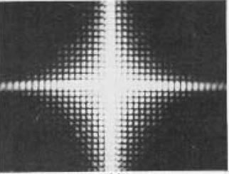
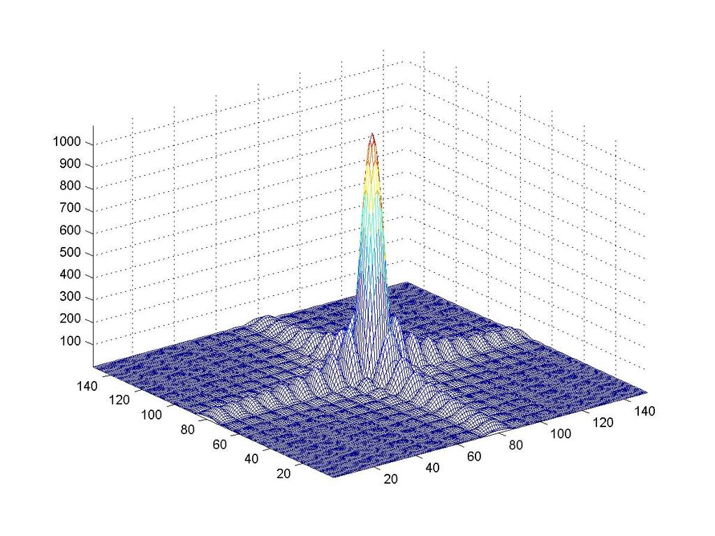
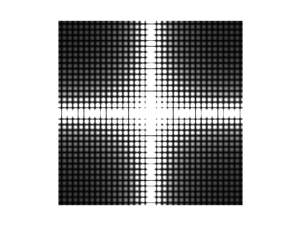
41 2D example no translation after translation 4

42 Going back to the intuition The FT decomposed the signal over its harmonic components and thus represents it as a sum of linearly independent complex exponential functions Thus, it can be interpreted as a mathematical prism 42

43 DFT Each term of the DFT, namely each value of F[k], results of the contributions of all the samples in the signal (f[n] for n=,..,n) The samples of f[n] are multiplied by trigonometric functions of different frequencies The domain over which F[k] lives is called frequency domain Each term of the summation which gives F[k] is called frequency component of harmonic component 43

44 DFT is a complex number F[k] in general are complex numbers [ ] = Re{ [ ]} + Im{ [ ]} [ ] = [ ] exp{ R [ ]} F k F k j F k F k F k j F k F k F k F k [ ] = Re{ [ ]} + Im{ [ ]} Im{ F[ k ]} R F[ k] = tan Re{ F[ k] } [ ] = Fk [ ] Pk magnitude or spectrum phase or angle power spectrum 44

45 Stretching vs shrinking stretched shrinked 45

46 Periodization vs discretization amplitude Linking continuous and discrete domains amplitude f k =f(kt s ) T s t n DT (discrete time) signals can be seen as sampled versions of CT (continuous time) signals Both CT and DT signals can be of finite duration or periodic There is a duality between periodicity and discretization Periodic signals have discrete frequency (sampled) transform Discrete time signals have periodic transform DT periodic signals have discrete (sampled) periodic transforms 46

47 Increasing the resolution by Zero Padding Consider the analysis formula [ ] = N F k N n=0 f [ n]e 2π jkn N If f[n] consists of N samples than F[k] consists of N samples as well, it is discrete (k is an integer) and it is periodic (because the signal f[n] is discrete time, namely n is an integer) The value of each F[k], for all k, is given by a weighted sum of the values of f[n], for n=,.., N- Key point: if we artificially increase the length of the signal adding M zeros on the right, we get a signal f [m] for which m=,,n+m-. Since f " $ [ m] = # $ % f [m] for 0 m < N 0 for N m < N + M 47

48 Increasing the resolution through ZP Then the value of each F[k] is obtained by a weighted sum of the real values of f[n] for 0 k N-, which are the only ones different from zero, but they happen at different normalized frequencies since the frequency axis has been rescaled. In consequence, F[k] is more densely sampled and thus features a higher resolution. 48

49 Increasing the resolution by Zero Padding 0 N 0 n zero padding F(Ω) (DTFT) in shade F[k]: sampled version 0 2π 2π/N 0 4π k 49

50 Zero padding zero padding Increasing the number of zeros augments the resolution of the transform since the samples of the DFT get closer 0 n N 0 F(Ω) 0 2π 2π/N 0 4π k 50

51 Summary of dualities SIGNAL DOMAIN FOURIER DOMAIN Sampling DTFT Periodicity Periodicity CTFS Sampling Sampling+Periodicity DTFS/DFT Sampling +Periodicity 5

52 Discrete Cosine Transform (DCT) Applies to digital (sampled) finite length signals AND uses only cosines. The DCT coefficients are all real numbers 52

53 Discrete Cosine Transform (DCT) Operate on finite discrete sequences (as DFT) A discrete cosine transform (DCT) expresses a sequence of finitely many data points in terms of a sum of cosine functions oscillating at different frequencies DCT is a Fourier-related transform similar to the DFT but using only real numbers DCT is equivalent to DFT of roughly twice the length, operating on real data with even symmetry (since the Fourier transform of a real and even function is real and even), where in some variants the input and/or output data are shifted by half a sample There are eight standard DCT variants, out of which four are common Strong connection with the Karunen-Loeven transform VERY important for signal compression 53

54 DCT DCT implies different boundary conditions than the DFT or other related transforms A DCT, like a cosine transform, implies an even periodic extension of the original function Tricky part First, one has to specify whether the function is even or odd at both the left and right boundaries of the domain Second, one has to specify around what point the function is even or odd In particular, consider a sequence abcd of four equally spaced data points, and say that we specify an even left boundary. There are two sensible possibilities: either the data is even about the sample a, in which case the even extension is dcbabcd, or the data is even about the point halfway between a and the previous point, in which case the even extension is dcbaabcd (a is repeated). 54

55 Symmetries 55

56 DCT N0 π Xk = xncos n+ k k 0,..., N0 n 0 N0 2 = = N0 2 π k xn = X0 + Xk cos k N0 2 + k = 0 N0 2 Warning: the normalization factor in front of these transform definitions is merely a convention and differs between treatments. Some authors multiply the transforms by (2/N 0 ) /2 so that the inverse does not require any additional multiplicative factor. Combined with appropriate factors of 2 (see above), this can be used to make the transform matrix orthogonal. 56

57 Summary of dualities SIGNAL DOMAIN FOURIER DOMAIN Sampling DTFT Periodicity Periodicity CTFS Sampling Sampling+Periodicity DTFS/DFT Sampling +Periodicity 57

58 Sampling From continuous to discrete time 58

59 Impulse Train Define a comb function (impulse train) as follows comb N [n] = δ[n ln ] l= where M and N are integers comb 2[ n] n 59

60 Impulse Train comb 2[ n] ( ) 2 comb u 2 2 n u 2 60

61 Impulse Train comb 2( x) ( ) 2 comb u 2 2 x u 2 2 6

62 Consequences Sampling (Nyquist) theorem 62

63 Sampling f( x) Fu ( ) comb M () x x x comb ( ) u M u u M M f() x comb () x M Fu ( )* comb ( u) M x 63 u

64 Sampling f( x) Fu ( ) x W W u f() x comb () x M Fu ( )* comb ( u) M x W u M Nyquist theorem: No aliasing if M > 2W M 64

65 Sampling f() x comb () x M Fu ( )* comb ( u) M x W u M M 2M If there is no aliasing, the original signal can be recovered from its samples by low-pass filtering. 65

66 Sampling f( x) Fu ( ) x W W u f() x comb () x M Fu ( )* comb ( u) M W u Aliased M 66

67 f( x) Sampling Fu ( ) Anti-aliasing filter x W W u f( x)* h( x) W W 2M u [ ] f( x)* h( x) comb ( x) M u M 67

68 Without anti-aliasing filter: Sampling f() x comb () x M W u With anti-aliasing filter: M [ ] f( x)* h( x) comb ( x) M u M 68

69 Images vs Signals D 2D Signals Frequency Temporal Spatial Time (space) frequency characterization of signals Reference space for Filtering Changing the sampling rate Signal analysis. Images Frequency Spatial Space/frequency characterization of 2D signals Reference space for Filtering Up/Down sampling Image analysis Feature extraction Compression. 69

70 2D Continuous FT 70

71 How do frequencies show up in an image? Low frequencies correspond to slowly varying information (e.g., continuous surface). High frequencies correspond to quickly varying information (e.g., edges) Original Image Low-passed 7

72 Large vertical frequencies correspond to horizontal lines 2D Frequency domain ω y Large horizontal and vertical frequencies correspond sharp grayscale changes in both directions Small horizontal and vertical frequencies correspond smooth grayscale changes in both directions ω x Large horizontal frequencies correspond to vertical lines 72

73 2D spatial frequencies 2D spatial frequencies characterize the image spatial changes in the horizontal (x) and vertical (y) directions Smooth variations -> low frequencies Sharp variations -> high frequencies y ω x = ω y =0 ω x =0 ω y = x 73

74 2D Continuous Fourier Transform 2D Continuous Fourier Transform (notation 2) + ˆ j 2π ( ux+ vy) f u, v f x, y e dxdy ( ) = ( ) + ˆ j 2π ( ux+ vy) f x y f u v e dudv (, ) (, ) = = 2 ˆ f( x, y) dxdy = f( u, v) dudv Plancherel s equality 2 74

75 Delta Sampling property of the 2D-delta function (Dirac s delta) Transform of the delta function δ ( x x, y y ) f( x, y) dxdy= f( x, y ) j2 π ( ux+ vy) { δ } δ F ( x, y) = ( x, y) e dxdy = j2 π ( ux+ vy) j π ux0+ vy0 { δ(, )} = δ(, ) = F x x y y x x y y e dxdy e ( ) shifting property 75

76 Constant functions Inverse transform of the impulse function j2 π( ux+ vy) j2 π(0x+ v0) { δ } F ( u, v) = δ( u, v) e dudv= e = Fourier Transform of the constant (= for all x and y) kxy (, ) = xy, j2 π ( ux+ vy) ( ) F u, v = e dxdy = δ ( u, v) 76

77 Trigonometric functions Cosine function oscillating along the x axis Constant along the y axis s( x, y) = cos(2 π fx) j2 π ( ux+ vy) { cos(2 π )} cos(2 π ) F fx = fx e dxdy = j2 π( fx) j2 π( fx) e + e = e 2 [ δ( u f) + δ( u+ f) ] j2 π ( ux+ vy) dxdy j2 π( u f ) x j2 π( u+ f ) x j2πvy = e + e e dxdy = 2 j2πvy j2 π( u f ) x j2 π( u+ f ) x j2 π( u f ) x j2 π( u+ f ) x e dy e e dx e e dx = 2 + = + =

78 Vertical grating ω y 0 ω x 78

79 Double grating ω y 0 ω x 79

80 Smooth rings ω y ω x 80

81 Vertical grating ω y -2πf 0 2πf ω x 8

82 2D box 2D sinc 82

83 CTFT properties Linearity Shifting Modulation Convolution Multiplication Separability af ( x, y) + bg( x, y) af( u, v) + bg( u, v) f x x y x e F u v j 2 π ( ux0 vy0 (, ) + ) (, ) 0 0 j2 π ( u0x+ v0y) e f x y F u u v v (, ) (, ) 0 0 f( x, y)* g( x, y) F( u, v) G( u, v) f( x, y) g( x, y) F( u, v)* G( u, v) f( x, y) = f( x) f( y) F( u, v) = F( u) F( v) 83

84 Separability. Separability of the 2D Fourier transform 2D Fourier Transforms can be implemented as a sequence of D Fourier Transform operations performed independently along the two axis j2 π ( ux+ vy) Fuv (, ) f( xye, ) dxdy j2πux j2πvy j2πvy j2πux f( x, y) e e dxdy e dy f( x, y) e dx j2πvy Fuye (, ) dy F uv, = = = = ( ) = = 2D FT D FT along the rows D FT along the cols 84

85 Separability Separable functions can be written as 2. The FT of a separable function is the product of the FTs of the two functions j2 π ( ux+ vy) Fuv (, ) f( xye, ) dxdy j2πux j2πvy j2πvy j2πux hxg ( ) ye e dxdy g ye dy hxe ( ) dx ( ) ( ) H u G v = = ( ) ( ) = = = (, ) = ( ) ( ) (, ) = ( ) ( ) f x y h x g y F u v H u G v (, ) = ( ) ( ) f x y f x g y 85

86 Discrete Time Fourier Transform (DTFT) Applies to Discrete domain signals and time series - 2D 86

87 Fourier Transform: 2D Discrete Signals Fourier Transform of a 2D discrete signal is defined as Fuv (, ) fmne [, ] = m= n= j2 π ( um+ vn) where uv, < 2 2 Inverse Fourier Transform /2 /2 j2 π ( um+ vn) f [ m, n] F( u, v) e dudv = /2 /2 87

88 Properties Periodicity: 2D Fourier Transform of a discrete a-periodic signal is periodic The period is for the unitary frequency notations and 2π for normalized frequency notations. Proof (referring to the firsts case) Fu ( + kv, + l) = fmne [, ] Arbitrary integers m= n= = m= n= = m= n= = Fuv (, ) ( ) j2 π ( u+ k) m+ ( v+ l) n ( ) j2π um+ vn j2πkm j2πln f[ m, n] e e e f[ m, n] e j2 π ( um+ vn) 88

89 Fourier Transform: Properties Linearity, shifting, modulation, convolution, multiplication, separability, energy conservation properties also exist for the 2D Fourier Transform of discrete signals. 89

90 DTFT Properties Linearity af [ m, n] + bg[ m, n] af( u, v) + bg( u, v) Shifting Modulation Convolution f m m n n e F u v j 2 π ( um0 vn0 [, ] + ) (, ) 0 0 j2 π ( u0m+ v0n) e f m n F u u v v [, ] (, ) 0 0 f[ m, n]* g[ m, n] F( u, v) G( u, v) Multiplication f[ m, n] g[ m, n] F( u, v)* G( u, v) Separable functions Energy conservation f[ m, n] = f[ m] f[ n] F( u, v) = F( u) F( v) 2 2 f[ m, n] = F( u, v) dudv m= n= 90

91 Fourier Transform: Properties Define Kronecker delta function δ[ mn, ], for m= 0 and n= 0 = 0, otherwise Fourier Transform of the Kronecker delta function ( ) π( ) j2π um+ vn j2 u0+ v0 Fuv (, ) = δ[ mne, ] = e = m= n= 9

92 Impulse Train Define a comb function (impulse train) as follows combm, N[ m, n] = δ[ m km, n ln] k= l= where M and N are integers comb 2[ n] n 92

93 Impulse Train k= l= comb M,N [m,n] δ[m km,n ln ] comb M,N (x, y) δ ( x km, y ln ) k= l= Fourier Transform of an impulse train is also an impulse train: k l δ[ m km, n ln] δ u, v MN = = M N k= l= k l comb, [ m, n] M N comb (,) u v, M N 93

94 Impulse Train comb 2[ n] ( ) 2 comb u 2 2 n u 2 94

95 comb M,N (x, y) = Impulse Train In the case of continuous signals: δ ( x km, y ln ) k= l= δ k l x km, y ln δ u, v MN = = M N ( ) k= l= k l comb, ( x, y) M N comb (,) u v, M N 95

96 Impulse Train comb 2( x) ( ) 2 comb u 2 2 x u

97 2D DTFT: constant Fourier Transform of f [k,l] =, k,l F[u,v] = k= l= $ j2π( uk+vl) e ' = %& () k= l= = δ(u k,v l) periodic with period along u and v To prove: Take the inverse Fourier Transform of the Dirac delta function and use the fact that the Fourier Transform has to be periodic with period. 97

98 Sampling theorem revisited 98

99 Sampling f( x) Fu ( ) comb M () x x x comb ( ) u M u u M M f() x comb () x M Fu ( )* comb ( u) M x 99 u

100 Sampling f( x) Fu ( ) x W W u f() x comb () x M Fu ( )* comb ( u) M x W u M Nyquist theorem: No aliasing if M > 2W M 00

101 Sampling f() x comb () x M Fu ( )* comb ( u) M x W u M M 2M If there is no aliasing, the original signal can be recovered from its samples by low-pass filtering. 0

102 Sampling f( x) Fu ( ) x W W u f() x comb () x M Fu ( )* comb ( u) M W u Aliased M 02

103 f( x) Sampling Fu ( ) Anti-aliasing filter x W W u f( x)* h( x) W W 2M u [ ] f( x)* h( x) comb ( x) M u M 03

104 Without anti-aliasing filter: Sampling f() x comb () x M W u With anti-aliasing filter: M [ ] f( x)* h( x) comb ( x) M u M 04

105 y Sampling in 2D (images) v f( x, y ) Fuv (, ) x W v W u u y comb, ( x, y) M N v comb (,) u v, M N x N u N M M 05

106 Sampling v W v f ( x, y) comb ( x, y) M, N u N M W u No aliasing if M > 2W u and N > 2W v 06

107 Interpolation (low pass filtering) v 2N u N Ideal reconstruction filter: M 2M MN, for u and v Huv (, ) = 2M 2N 0, otherwise 07

108 Anti-Aliasing a=imread( barbara.tif ); 08

109 Anti-Aliasing a=imread( barbara.tif ); b=imresize(a,0.25); c=imresize(b,4); 09

110 Anti-Aliasing a=imread( barbara.tif ); b=imresize(a,0.25); c=imresize(b,4); H=zeros(52,52); H(256-64:256+64, :256+64)=; Da=fft2(a); Da=fftshift(Da); Dd=Da.*H; Dd=fftshift(Dd); d=real(ifft2(dd)); 0

Contents. Signals as functions (1D, 2D)

Contents. Signals as functions (1D, 2D) Fourier Transform The idea A signal can be interpreted as en electromagnetic wave. This consists of lights of different color, or frequency, that can be split apart usign an optic prism. Each component