Overview. Signals as functions (1D, 2D) 1D Fourier Transform. 2D Fourier Transforms. Discrete Fourier Transform (DFT) Discrete Cosine Transform (DCT)

Transcription

1 Fourier Transform

2 Overview Signals as functions (1D, 2D) Tools 1D Fourier Transform Summary of definition and properties in the different cases CTFT, CTFS, DTFS, DTFT DFT 2D Fourier Transforms Generalities and intuition Examples A bit of theory Discrete Fourier Transform (DFT) Discrete Cosine Transform (DCT)

3 Signals as functions 1. Continuous functions of real independent variables 1D: f=f(x) 2D: f=f(x,y) x,y Real world signals (audio, ECG, images) 2. Real valued functions of discrete variables 1D: f=f[k] 2D: f=f[i,j] Sampled signals 3. Discrete functions of discrete variables 1D: y=y[k] 2D: y=y[i,j] Sampled and quantized signals For ease of notations, we will use the same notations for 2 and 3

4 Images as functions Gray scale images: 2D functions Domain of the functions: set of (x,y) values for which f(x,y) is defined : 2D lattice [i,j] defining the pixel locations Set of values taken by the function : gray levels Digital images can be seen as functions defined over a discrete domain {i,j: 0<i<I, 0<j<J} I,J: number of rows (columns) of the matrix corresponding to the image f=f[i,j]: gray level in position [i,j]

5 Example 1: δ function [ ] = = = j i j i j i j i 0;, 0 0 1, δ [ ] = = = otherwise J j i J j i 0 0; 1, δ

6 Example 2: Gaussian Continuous function f x + y 1 2 2σ (, ) x y = σ e 2π 2 2 Discrete version f i + j 1 2 2σ [ i, j] = e σ 2π 2 2

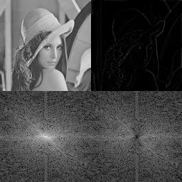
7 Example 3: Natural image

8 Example 3: Natural image

9 Fourier Transform Different formulations for the different classes of signals Summary table: Fourier transforms with various combinations of continuous/discrete time and frequency variables. Notations: CTFT: continuous time FT: t is real and f real (f=ω) (CT, CF) DTFT: Discrete Time FT: t is discrete (t=n), f is real (f=ω) (DT, CF) CTFS: CT Fourier Series (summation synthesis): t is real AND the function is periodic, f is discrete (f=k), (CT, DF) DTFS: DT Fourier Series (summation synthesis): t=n AND the function is periodic, f discrete (f=k), (DT, DF) P: periodical signals T: sampling period ω s : sampling frequency (ω s =2π/T) For DTFT: T=1 ω s =2π

10 Continuous Time Fourier Transform (CTFT) Time is a real variable (t) Frequency is a real variable (ω)

11 CTFT: Concept A signal can be represented as a weighted sum of sinusoids. Fourier Transform is a change of basis, where the basis functions consist of sins and cosines (complex exponentials). [Gonzalez Chapter 4]

12 Continuous Time Fourier Transform (CTFT) T=1

13 Fourier Transform Cosine/sine signals are easy to define and interpret. However, it turns out that the analysis and manipulation of sinusoidal signals is greatly simplified by dealing with related signals called complex exponential signals. A complex number has real and imaginary parts: z = x+j y A complex exponential signal: ( α α ) jα re = r cos + jsin

14 CTFT Continuous Time Fourier Transform Continuous time a-periodic signal Both time (space) and frequency are continuous variables NON normalized frequency ω is used Fourier integral can be regarded as a Fourier series with fundamental frequency approaching zero Fourier spectra are continuous A signal is represented as a sum of sinusoids (or exponentials) of all frequencies over a continuous frequency interval Fourier integral ( ω) = () jωt F f t e dt t 1 jωt f() t = F( ω) e dω 2π ω analysis synthesis

15 Then CTFT becomes Fourier Transform of a 1D continuous signal j2πux F( u) f ( xe ) dx = Euler s formula ( π ) ( π ) j2πux e = cos 2 ux jsin 2 ux Inverse Fourier Transform 2 f( x) F( u) e j πux du =

16 CTFT: change of notations Fourier Transform of a 1D continuous signal Euler s formula jωx F( ω) = f( x) e dx Inverse Fourier Transform 1 jωx f( x) = F( ω) e dω 2π ( ω ) sin ( ω ) jωx e = cos x j x Change of notations: ω 2π u ωx 2π u ω y 2π v

17 CTFT Replacing the variables j2πux F(2 πu) F( u) f( x) e dx More compact notations = = = 1 j2πux j2πux ( π ) f( x) = F( u) e d 2 u = F( u) e du 2π j2πux Fu ( ) = f( xe ) dx j2πux f x = F( u) e du ( )

18 Sinusoids Frequency domain characterization of signals + jωt F( ω) = f( te ) dt Signal domain Frequency domain (spectrum, absolute value of the transform)

19 Time domain Gaussian Frequency domain

20 rect Time domain Frequency domain sinc function

21 Example

22 Example

23 Discrete Fourier Transform (DFT) The easiest way to get to it Time is a discrete variable (t=n) Frequency is a discrete variable (f=k)

24 DFT The DFT can be considered as a generalization of the CTFT to discrete series N 1 1 j 2 π kn / N Fk [ ] = f[ ne ] N n= 0 N 1 f[ n] = F[ k] e k = 0 n= 0,1,, N 1 k = 0,1,, N 1 In order to calculate the DFT we start with k=0, calculate F(0) as in the formula below, then we change to u=1 etc F[0] is the average value of the function f[n] 0 This is also the case for the CTFT j2 π kn/ N N 1 N 1 1 j2π 0 n/ N 1 F[0] = f[ ne ] = f[ n] = f N N n= 0 n= 0

25 Example 1 amplitude 0 time F[k] F[0] low-pass characteristic frequency

26 Example 2 amplitude 0 time F[k] F[0]=0 band-pass (or high-pass) characteristic -M 0 M frequency

27 DFT About M 2 multiplications are needed to calculate the DFT The transform F[k] has the same number of components of f[n], that is N The DFT always exists for signals that do not go to infinity at any point Using the Eulero s formula N 1 N 1 1 j2 π kn/ N 1 F[ k] = f[ ne ] = f[ n] cos j2 kn/ N jsin j2 kn/ N N N n= 0 n= 0 ( ( π ) ( π )) frequency component k discrete trigonometric functions

28 Intuition The FT decomposed the signal over its harmonic components and thus represents it as a sum of linearly independent complex exponential functions Thus, it can be interpreted as a mathematical prism

29 DFT is a complex number F[k] in general are complex numbers [ ] = Re{ [ ]} + Im{ [ ]} [ ] = [ ] exp{ [ ]} F k F k j F k F k F k j F k F k F k F k [ ] = Re{ [ ]} + Im{ [ ]} Im{ F[ k 1 ]} F[ k] = tan Re{ F[ k] } [ ] = Fk [ ] Pk magnitude or spectrum phase or angle power spectrum

30 Example

31 Let s take a bit more advanced perspective Book: Lathi, Signal Processing and Linear Systems

32 Overview Transform Time Frequency Analysis/Synthesis Duality (Continuous Time) Fourier Transform (CTFT) (Continuous Time) Fourier Series (CTFS) Discrete Time Fourier Transform (DTFT) C C jωt F ω = f t e dt Self-dual C P D D C P ( ) () t 1 jωt f () t = F( ω) e dω 2π ω T /2 1 j2 π kt/ T Fk [ ] = f ( te ) dt T T /2 f() t = F[ k] e k + 2π j2 π kt/ T F( Ω ) = f[ k] e k = jωk 1 jωk f [ k] = F( Ω) e dω 2π Dual with DTFT Dual with CTFS Discrete Time Fourier Series (DTFS) D P D P N 1 1 Fk [ ] = f[ ne ] N n= 0 N 1 f[ n] = F[ k] e n= 0 j2 π kn / T j2 π kn/ T Self dual

33 Linking continuous and discrete domains amplitude amplitude f k =f(kt s ) T s t n DT signals can be seen as sampled versions of CT signals Both CT and DT signals can be of finite duration or periodic There is a duality between periodicity and discretization Periodic signals have discrete frequency (DF) transform (f=k) CTFS Discrete time signals have periodic transform DTFT DT periodic signals have DF periodic transforms DTFS, DFT

34 Dualities SIGNAL DOMAIN FOURIER DOMAIN Sampling DTFT Periodicity Periodicity CTFS Sampling Sampling+Periodicity DTFS/DFT Sampling +Periodicity

35 Sequences of samples f[k]: sample values Assumes a unitary spacing among samples (T s =1) Normalized frequency Ω Transform DTFT for NON periodic sequences CTFS for periodic sequences DFT for periodized sequences All transforms are 2π periodic 2π Ω s = ωsts = Ts = 2π T Discrete time signals s Ω = ωt s Sampled signals f(kt s ): sample values The sampling interval (or period) is T s Non normalized frequency ω Transform DTFT CSTF DFT BUT accounting for the fact that the sequence values have been generated by sampling a real signal f k =f(kt s ) All transforms are periodic with period ω s 2π ω = s T s

36 Connection DTFT-CTFT sampling periodization Fc(ω) f(t) t 0 _ Fc(ω) ω f(kt s ) f[k] 0Ts 4Ts t 0 F(Ω) 2π/Ts ω k 0 2π Ω

37 CTFS Continuous Time Fourier Series Continuous time periodic signals The signal is periodic with period T The transform is sampled (it is a series) amplitude T t T /2 1 j2 π kt/ T F k = f te dt [ ] ( ) T T /2 f() t = F[ k] e k j2 π kt/ T coefficients of the Fourier series periodic signal

38 CTFS Representation of a continuous time signal as a sum of orthogonal components in a complete orthogonal signal space The exponentials are the basis functions Properties even symmetry only cosinusoidal components odd symmetry only sinusoidal components

39 DTFT Discrete Time Fourier Transform Discrete time a-periodic signal The transform is periodic and continuous with period non normalized frequency ω = s 2π T s n ( ω) F = f ne = f ne j2 πωn/ ωs jωnt [ ] [ ] n n ωs /2 π / T j πωn ω π jωnt s 1 jωt 2 / 2 s jωt s f [ n] = F( e ) e dω F( e ) e dω ω = s T ωs /2 s π / Ts 2π 2πω 2πω ωs = = Ts = ωts T ω 2π s s s T s = 2 π / ω s sampling interval in time periodicity in frequency the closer the samples, the farther the replicas

40 DTFT with normalized frequency Normalized frequency: change of variables Ω = ωt s 2π Ω s = ωsts = Ts = Ts Ω = 2π s 2π normalized frequency periodicity in the normalized frequency domain + F( Ω ) = f[ k] e n= 1 jkω f [ n] = F( Ω) e dω 2π F ( ) 2π 1 Ω Ω = Fc T s T s jnω Relation to the CTFT If Ts>1, the DTFT can be seen as a stretched periodized version of the CTFT.

41 DTFT with normalized frequency F(Ω) can be _ obtained from F c (ω) by replacing ω with Ω /T s. Thus F(Ω) is identical to F(ω) frequency scaled and stratched by a factor 1/T s, where T s is the sampling interval in time domain Notations DTFT 1 Ω F( Ω ) = Fc T s T s 2π 2π ωs = Ts = T ω s s Ω ω = Ω = ωt T ( ω ) ( ω π ω ) F( Ω) F T = F 2 / s s s CTFT periodicity of the spectrum normalized frequency (the spectrum is 2π-periodic) s + + jωn j2 nπω/ ωs ( Ω ) = [ ] ( ω s ) = ( ω) = [ ] n= k= F f ne F T F f ne

42 DTFT with unitary frequency ( f ) Ω= 2π u ω = 2π jωn j2π nu F( Ω ) = f[ n] e F( u) = f[ n] e n= 1 2 jωn j2πnu j2πnu 1 f [ n] = F( Ω) e dω f[ n] = F( u) e du = F( u) e du 2π Fu ( ) = fke [ ] n= [ ] = ( ) 2π 1 j2π nu 1 2 j2π nu f n F u e du 1 2 n= 1 2 NOTE: when T s =1, Ω=ω and the spectrum is 2π-periodic. The unitary frequency u=2π/ Ω corresponds to the signal frequency f=2π/ω. This could give a better intuition of the transform properties.

43 Summary Sampled signals are sequences of sampels Looking at the sequence as to a set of samples obtained by sampling a real signal with sampling frequency ω s we can still use the formulas for calculating the transforms as derived for the sequences by Stratching the time axis (and thus squeezing the frequency axis if T s >1) normalized frequency (sample series) spectral periodicity in Ω Ω = ωt 2π ω = s s 2π T s frequency (sampled signal) spectral periodicity in ω Enclosing the sampling interval T s in the value of the sequence samples (DFT) f ( ) = Tf kt k s s

44 Connection DTFT-CTFT sampling periodization Fc(ω) f(t) t 0 _ Fc(ω) ω f(kt s ) f[k] 0Ts 4Ts t 0 F(Ω) 2π/Ts ω k 0 2π Ω

45 Differences DTFT-CTFT The DTFT is periodic with period Ω s =2π (or ω s =2π/T s ) The discrete-time exponential e jωn has a unique waveform only for values of Ω in a continuous interval of 2π Numerical computations can be conveniently performed with the Discrete Fourier Transform (DFT)

46 DTFS Discrete Time Fourier Series Discrete time periodic sequences of period N 0 Fundamental frequency Ω = 2 π /N 0 0 N0 1 1 Fk [ ] = f[ ne ] N N 0 k = 0 0 n= 0 1 jkn2 π / N f[ n] = F[ k] e jkn2 π / N 0 0

47 DTFS: Example N 0 =20 T s =1 Ω s =2π Ω 0 = π/10 [Lathi, pag 621]

48 Discrete Fourier Transform (DFT) N0 N0 j nk jnω0k N0 Fk [ ] = fe = fe n n= 0 n= 0 0 N0 N0 jn k jnω0k N0 The DFT transforms N 0 samples of a discrete-time signal to the same number of discrete frequency samples The DFT and IDFT are a self-contained, one-to-one transform pair for a length-n 0 discrete-time signal (that is, the DFT is not merely an approximation to the DTFT as discussed next) However, the DFT is very often used as a practical approximation to the DTFT 2π f[ n] = F[ k] e = F[ k] e N N Ω = 2π N 0 k= 0 0 k= 0 n 2π

49 DFT 0 N 0 n zero padding F(Ω) 0 2π 2π/N 0 4π k

50 zero padding DFT Increasing the number of zeros augments the resolution of the transform since the samples of the DFT gets closer 0 N 0 F(Ω) n 0 2π 2π/N 0 4π k

51 Properties For real signals f(t) ( ) fˆ ( ω) ( ) ˆ( ) ˆ ω = ( ω) f t f t f f Proof + + jωt jωt' { f ( t) } f ( t) e dt f ( t' ) e dt' fˆ ( ω) I = = =

52 Discrete Cosine Transform (DCT) Operate on finite discrete sequences (as DFT) A discrete cosine transform (DCT) expresses a sequence of finitely many data points in terms of a sum of cosine functions oscillating at different frequencies DCT is a Fourier-related transform similar to the DFT but using only real numbers DCT is equivalent to DFT of roughly twice the length, operating on real data with even symmetry (since the Fourier transform of a real and even function is real and even), where in some variants the input and/or output data are shifted by half a sample There are eight standard DCT variants, out of which four are common Strong connection with the Karunen-Loeven transform VERY important for signal compression

53 DCT DCT implies different boundary conditions than the DFT or other related transforms A DCT, like a cosine transform, implies an even periodic extension of the original function Tricky part First, one has to specify whether the function is even or odd at both the left and right boundaries of the domain Second, one has to specify around what point the function is even or odd In particular, consider a sequence abcd of four equally spaced data points, and say that we specify an even left boundary. There are two sensible possibilities: either the data is even about the sample a, in which case the even extension is dcbabcd, or the data is even about the point halfway between a and the previous point, in which case the even extension is dcbaabcd (a is repeated).

54 Symmetries

55 DCT N0 1 π 1 Xk = xn cos n+ k k 0,..., N0 1 n 0 N0 2 = = N π k 1 xn = X0 + Xk cos k N0 2 + k = 0 N0 2 Warning: the normalization factor in front of these transform definitions is merely a convention and differs between treatments. Some authors multiply the transforms by (2/N 0 ) 1/2 so that the inverse does not require any additional multiplicative factor. Combined with appropriate factors of 2 (see above), this can be used to make the transform matrix orthogonal.

56 Images vs Signals 1D 2D Signals Frequency Temporal Spatial Time (space) frequency characterization of signals Reference space for Filtering Changing the sampling rate Signal analysis. Images Frequency Spatial Space/frequency characterization of 2D signals Reference space for Filtering Up/Down sampling Image analysis Feature extraction Compression.

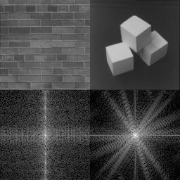
57 2D spatial frequencies 2D spatial frequencies characterize the image spatial changes in the horizontal (x) and vertical (y) directions Smooth variations -> low frequencies Sharp variations -> high frequencies y ω x =1 ω y =0 ω x =0 ω y =1 x

58 Large vertical frequencies correspond to horizontal lines 2D Frequency domain ω y Large horizontal and vertical frequencies correspond sharp grayscale changes in both directions Small horizontal and vertical frequencies correspond smooth grayscale changes in both directions ω x Large horizontal frequencies correspond to vertical lines

59 Vertical grating ω y 0 ω x

60 Double grating ω y 0 ω x

61 Smooth rings ω y ω x

62 2D box 2D sinc

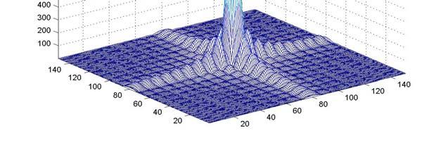
63 Margherita Hack log amplitude of the spectrum

64 Einstein log amplitude of the spectrum

65 What we are going to analyze 2D Fourier Transform of continuous signals (2D-CTFT) 1D + + ( ) ( ) j ω t jωt F ω = f te dt, f ( t) = F( ω) e dt 2D Fourier Transform of discrete space signals (2D-DTFT) 1D jωk 1 jωk F( Ω ) = f[ ke ], f [ k] = F( Ω) e dt 2π k = 2π 2D Discrete Fourier Transform (2D-DFT) 1D N 1 N 1 1 2π F = f k e f k = Fe Ω = 0 0 jrω0k jrω0k [], [], 0 r N r 0 k= 0 N0 r= 0 N0

66 2D Continuous Fourier Transform Continuous case (x and y are real) 2D-CTFT (notation 1) ( ωx ωy) = ( ) j ˆ ( ωxx+ ωyy) f, f x, y e dxdy 1 j( ω ) ( ) ˆ xx+ ωyy f xy, = f 2 (, ) e d d 4 π + + ω ω ω ω x y x y * 1 * f ( xyg, ) ( xydxdy, ) = fˆ 2 ( ωx, ωy) gˆ ( ωx, ωy) dωxdωy 4π f = g f ( x, y) dxdy fˆ = 2 ( ωx, ωy) dωxdωy 4π Parseval formula Plancherel equality

67 2D Continuous Fourier Transform Continuous case (x and y are real) 2D-CTFT ωx = 2π u ω = 2πv y + j2π ( ux+ vy) f u v f x y e dxdy ( ) = ( ) ˆ,, + 1 ˆ j2π,, 2 2 4π ( ) ( ) ( ux+ vy ) ( π ) f x y = f u v e dudv = = + 1 ˆ j2π 2 f ( u, v) e 2 4π ( ux+ vy ) ( π ) 2 2 dudv

68 2D Continuous Fourier Transform 2D Continuous Fourier Transform (notation 2) + j2π ( ux+ vy) f u v f x y e dxdy ( ) = ( ) ˆ,, + j2π ( ux+ vy) f x y f u v e dudv (, ) ˆ (, ) = = 2 ˆ f ( x, y) dxdy = f ( u, v) dudv Plancherel s equality 2

69 2D Discrete Fourier Transform The independent variable (t,x,y) is discrete F r 0 = N 1 0 k = 0 0 f[ k] e N0 1 1 fn [ k] = Fe 0 r N Ω = 2π N 0 jrω k r = 0 0 jrω k N Fuv [, ] = f[ ike, ] i= 0 k= u= 0 v= 0 jω ( ui+ vk) N0 1N0 1 1 fn [, i k] = F[ u, v] e 0 N Ω = 2π N N 0 jω ( ui+ vk ) 0 [Lathi s notations]

70 Delta Sampling property of the 2D-delta function (Dirac s delta) Transform of the delta function δ ( x x, y y ) f( x, y) dxdy = f( x, y ) j2 π ( ux+ vy) { δ } δ F ( x, y) = ( x, y) e dxdy = 1 j2 π ( ux+ vy) j π ux0+ vy0 { δ(, )} = δ(, ) = F x x y y x x y y e dxdy e ( ) shifting property

71 Constant functions Inverse transform of the impulse function 1 j2 π( ux+ vy) j2 π(0x+ v0) { δ } F ( u, v) = δ( u, v) e dudv = e = 1 Fourier Transform of the constant (=1 for all x and y) kxy (, ) = 1 xy, j2 π ( ux+ vy) ( ) F uv, = e dxdy= δ ( uv, )

72 Trigonometric functions Cosine function oscillating along the x axis Constant along the y axis sxy (, ) = cos(2 π fx) j2 π ( ux+ vy) { cos(2 π )} cos(2 π ) F fx = fx e dxdy = j2 π( fx) j2 π( fx) e + e = e 2 [ δ( u f) + δ( u+ f) ] j2 π ( ux+ vy) dxdy 1 j2 π( u f ) x j2 π( u+ f ) x j2πvy = e + e e dxdy = 2 j2πvy j2 π( u f ) x j2 π( u+ f ) x j2 π( u f ) x j2 π( u+ f ) x e dy e e dx e e dx 1 1 = = + = 2 1 2

73 Vertical grating ω y -2πf 0 2πf ω x

74 Ex. 1

75 Ex. 2

76 Ex. 3 Magnitudes

77 Examples

78 Properties Linearity Shifting Modulation Convolution Multiplication Separability af ( x, y) + bg( x, y) af( u, v) + bg( u, v) f x x y x e F u v j 2 π ( ux0 vy0 (, ) + ) (, ) 0 0 j2 π ( u0x+ v0y) e f x y F u u v v (, ) (, ) 0 0 f ( xy, )* gxy (, ) FuvGuv (, ) (, ) f ( xygxy, ) (, ) Fuv (, )* Guv (, ) f ( xy, ) = f( xf ) ( y) Fuv (, ) = FuFv ( ) ( )

79 Separability 1. Separability of the 2D Fourier transform 2D Fourier Transforms can be implemented as a sequence of 1D Fourier Transform operations performed independently along the two axis j2 π ( ux+ vy) Fuv (, ) f( xye, ) dxdy j2πux j2πvy j2πvy j2πux f ( x, y) e e dxdy e dy f ( x, y) e dx ( ) j2π vy (, ), = Fuye dy= F uv = = = = 2D DFT 1D DFT along the rows 1D DFT along the cols

80 Separability Separable functions can be written as 2. The FT of a separable function is the product of the FTs of the two functions j2 π ( ux+ vy) Fuv (, ) f( xye, ) dxdy j2πux j2πvy j2πvy j2πux h( x) g y e e dxdy g y e dy h( x) e dx ( ) ( ) H u G v = = ( ) ( ) = = = (, ) = ( ) ( ) (, ) = ( ) ( ) f x y h x g y F u v H u G v (, ) = ( ) ( ) f xy f xg y

81 2D Fourier Transform of a Discrete function Fourier Transform of a 2D a-periodic signal defined over a 2D discrete grid The grid can be thought of as a 2D brush used for sampling the continuous signal with a given spatial resolution (T x,t y ) 1D jωk 1 jωk F( Ω ) = f[ k] e, f[ k] = F( Ω) e dt 2π k = 2π 2D F( Ω, Ω ) = f[ k, k ] e x y ( 1 x k2 y) 1 jk ( 1Ω x+ k2ωy) f[ k] = F( Ω, Ω ) e dω Ω 2 4 π 2π 2π + + k = k = jkω + Ω x y x y Ω x,ω y : normalized frequency

82 Unitary frequency notations Ω x = 2π u Ω y = 2π v Fuv (, ) = fk [, k] e 1 2 1/2 1/2 1 2 j2 π ( k u+ k v) 1 2 j2 π ( k1u+ k2v) f k k F u v e dudv [, ] = (, ) 1 2 k + + = k = 1/2 1/2 The integration interval for the inverse transform has width=1 instead of 2π It is quite common to choose 1 1 uv, < 2 2

83 Properties Periodicity: 2D Fourier Transform of a discrete a-periodic signal is periodic The period is 1 for the unitary frequency notations and 2π for normalized frequency notations. Proof (referring to the firsts case) Fu ( + kv, + l) = fmne [, ] Arbitrary integers m= n= = m= n= = m= n= = F( uv, ) ( ) j 2 π ( u+ k) m+ ( v+ l) n ( ) j2π um+ vn j2π km j2πln f[ m, n] e e e f[ m, n] e j 2 π ( um+ vn) 1 1

84 Properties Linearity shifting modulation convolution multiplication separability energy conservation properties also exist for the 2D Fourier Transform of discrete signals. NOTE: in what follows, (k 1,k 2 ) is replaced by (m,n)

85 2D DTFT Properties Linearity Shifting Modulation af [ m, n] + bg[ m, n] af( u, v) + bg( u, v) f m m n n e F u v j 2 π ( um0 vn0 [, ] + ) (, ) 0 0 j2 π ( u0m+ v0n) e f m n F u u v v [, ] (, ) 0 0 Convolution Multiplication f [ mn, ]* g[ mn, ] FuvGuv (, ) (, ) f [ mngmn, ] [, ] Fuv (, )* Guv (, ) Separable functions Energy conservation f [ m, n] = f[ m] f[ n] F( u, v) = F( u) F( v) 1/2 1/2 2 2 f [ mn, ] = Fuv (, ) dudv m= n= 1/2 1/2

86 Impulse Train Define a comb function (impulse train) as follows combm, N[ m, n] = δ[ m km, n ln] k= l= where M and N are integers 1 comb [ n] 2 n

87 Appendix

88 2D-DTFT: delta Define Kronecker delta function δ[ mn, ] 1, for m= 0 and n= 0 = 0, otherwise DT Fourier Transform of the Kronecker delta function j2π( um+ vn) j2π( u0+ v0 ) = = = Fuv (, ) δ[ mne, ] e 1 m= n=

89 2D DT Fourier Transform: constant Fourier Transform of 1 f[ k, l] = 1, k, l j2π ( uk+ vl ) = = Fuv [, ] 1e k= l= = δ ( u k, v l) k= l= periodic with period 1 along u and v To prove: Take the inverse Fourier Transform of the Dirac delta function and use the fact that the Fourier Transform has to be periodic with period 1.