CRAIG HICKMAN. B.S., Kansas State University, 2004 A THESIS MASTER OF SCIENCE. KANSAS STATE UNIVERSITY Manhattan, Kansas

Transcription

1 Determining the Effects of Duct Fittings on Volumetric Air flow Measurements by CRAIG HICKMAN B.S., Kansas State University, 24 A THESIS submitted in partial fulfillment of the requirements for the degree MASTER OF SCIENCE Department of Mechanical and Nuclear Engineering College of Engineering KANSAS STATE UNIVERSITY Manhattan, Kansas 21 Approved by: Major Professor B. Terry Beck

2 Abstract The purpose of the research was to quantify the influence of several duct disturbances on volumetric flow rate measurements and use these in developing guidelines for field technicians. This will assist the field technicians in making more accurate volumetric air flow measurements in rectangular ducts during a test and balance operation. Multiple duct sizes, fittings, probes, traverse algorithms, and locations upstream and downstream of the disturbances are used to compare a variety of situations. The two traverse algorithms used are the log-tchebycheff and equal area methods. Two upstream and five downstream locations are tested for each duct configuration. Two air velocity probes are used for local velocity measurements on each traverse: a pitot-static probe and a hot wire anemometer. A nozzle bank and Air Flow Measurement Station are used as the flow measurement standards for comparison with each traverse. This paper discusses the setup and initial results of ASHRAE 1245-RP. Data collected subsequent to this thesis will complete the balance of results and will be collected and analyzed by other researchers. Results will be summarized and presented in a way which allows technicians to use it in the field for more accurate balancing results.

3 Table of Contents List of Figures... vii List of Tables... x Acknowledgements... xi CHAPTER 1 - Introduction Background and Relevant Literature Testing... 2 CHAPTER 2 - Experimental Facility Blower Nozzle Bank Flow Measurement Standard Air Flow Measurement Station (FMS) Duct Configurations and Fabrication CHAPTER 3 - Flow Rate Determination Air Properties Barometric Pressure Temperature Humidity Air Density Accuracy Verification Standard Air Density Nozzle Bank Flow Measurement Standard Nozzle Expansion Factor Nozzle Discharge Coefficient Static Pressure Air Flow Measurement Station Flow Measurement by Duct Traverses chebycheff and Algorithms Measurement Plane Locations Local Air Velocity Measurements Pitot-static Probe iii

4 Thermal Anemometer Correction to Standard Air Density CHAPTER 4 - Experimental Procedure Nozzle Chamber Measurement Procedure Flow Measurement Station Procedure Traverse Measurement Procedure Probe Positioning Procedure Probe Specification Compliance Procedure CHAPTER 5 - Experimental Uncertainty Air Property Uncertainties Nozzle Bank Flow Uncertainty Nozzle Expansion Factor Uncertainty Discharge Coefficient Uncertainty Nozzle Area Uncertainty Traversing Algorithm Uncertainties Duct Area Uncertainty Traverse Methods Flow Measurement Station Uncertainty... 5 CHAPTER 6 - Experimental Data and Analysis No Disturbance (Straight Duct) Analysis Single Flow Path Disturbance Analysis Multiple Flow Path (Tee) Disturbance Analysis CHAPTER 7 - Conclusions References Appendix A - Seal Test... 7 A.1 Duct Sealing Procedure... 7 A.2 Seal Test Procedure... 7 A.3 Duct Leakage Measurement A.4 Leakage Check for Tee A.5 Seal Test Conclusions Appendix B - Data iv

5 B.1 Data (24 x 24 Upstream Duct Size, No Disturbance) B.2 Data (24 x 24 Upstream Duct Size, 6 Transition) B.3 Data (24 x 24 Upstream Duct Size, 9 Transition) B.4 Data (24 x 24 Upstream Duct Size, 9 Elbow) B.5 Data (24 x 24 Upstream Duct Size, 9 Tee) Appendix C - Calibrations C.1 Pressure Transducer Calibrations C.1.1 Nozzle Chamber Pressure Transducers C.1.2 FMS Pressure Transducers C.2 FMS Calibration C.3 Humidity Sensor Calibration Appendix D - Instrument Specifications... 1 Appendix E - Example Calculations E.1 Example Data E.1.1 Example 1 Data E.1.2 Example 2 Data E.2 Example Air Property Calculations E.2.1 Example Air Viscosity Calculation E.2.2 Example Air Density Calculation E.3 Example Nozzle Bank Flow Rate Calculations E.3.1 Example Alpha Ratio Calculation E.3.2 Example Beta Ratio Calculation E.3.3 Example Nozzle Expansion Factor Calculation E.3.4 Example Nozzle Discharge Coefficient Calculation E.3.5 Example Volumetric Air Flow Rate Calculation E.4 Example 1 Traverse Flow Rate and Error Calculations E.4.1 Example 1 Traverse Flow Rate Calculation E.4.2 Example 1 Traverse Error Calculation E.5 Example FMS Calculation E.6 Example 2 Traverse Flow Rate and Error Calculations E.6.1 Example 2 Traverse Flow Rate Calculation v

6 E.6.2 Example 2 Traverse Error Calculation Appendix F - LabView Files F.1 LabView Front Panels F.2 LabView Block Diagrams vi

7 List of Figures Figure 2.1 General Test Area (a) Transitions and (b) Elbows... 5 Figure 2.2 General Test Area (Tees)... 6 Figure 2.3 General Test Site Figure 2.4 General Test Site Figure 2.5 Nozzle Chamber based on (Heber et al., 1991)... 1 Figure 2.6 Pressure Tap based on (Heber et al., 1991) Figure 2.7 Nozzle Layout based on (Heber et al., 1991) Figure 2.8 Altered Nozzle Chamber Figure 2.9 Nozzle Chamber Figure 2.1 Nozzle Chamber Figure 2.11 Nozzle Bank Figure 2.12 FMS Figure 2.13 FMS Figure 2.14 Tee Figure 3.1 Pitot-static Probe Figure 3.2 EBT 72 Electronic Balancing Tool Figure 3.3 EBT 72 Reduction in Random Uncertainty Figure 3.4 TSI VelociCalc Model 8347 Anemometer Figure 4.1 Pitot-static Probe Setup Figure 4.2 Pitot-static Probe Picture Figure 4.3 Pitot-static Probe Picture Figure 4.4 Anemometer Setup Figure 5.1 FMS Flow Coefficient Calibration Curve Figure 5.2 FMS Calibration Coefficient Deviation Plot Figure o Elbow Data Sheet page Figure o Elbow Data Sheet page Figure 6.3 Velocity Profiles 3 De Upstream vii

8 Figure 6.4 Velocity Profiles 7.5 De Downstream Figure 6.5 No Disturbance 12 SFPM Data Example Figure Transition 12 SFPM Data Example Figure Transition 12 SFPM Data Example... 6 Figure Elbow 12 SFPM Data Example... 6 Figure 6.9 Pitot Probe Flow Coefficient Variation Figure Tee Qb/Qc =.2 Datasheet Figure Tee Qb/Qc =.2 Datasheet Figure Tee Qb/Qc =.2 12 SFPM Data Example Figure Tee, Qb/Qc =.4, 12 SFPM Data Example Figure Tee, Qb/Qc =.6, 12 SFPM Data Example Figure A.1 End Cap Figure A.2 Leakage Fluctuations Figure A.3 Duct Leakage for Tee Figure B.1 Data - No Disturbance, 6 fpm Figure B.2 Data - No Disturbance, 12 fpm Figure B.3 Data - No Disturbance, 18 fpm Figure B.4 Data - No Disturbance, 24 fpm Figure B.5 Data - 6 Transition, 6 fpm Figure B.6 Data - 6 Transition, 12 fpm Figure B.7 Data - 6 Transition, 18 fpm Figure B.8 Data - 6 Transition, 24 fpm Figure B.9 Data - 9 Transition, 6 fpm Figure B.1 Data - 9 Transition, 12 fpm... 8 Figure B.11 Data - 9 Transition, 18 fpm... 8 Figure B.12 Data - 9 Transition, 24 fpm Figure B.13 Data - 9 Elbow, 6 fpm Figure B.14 Data - 9 Elbow, 12 fpm Figure B.15 Data - 9 Elbow, 18 fpm Figure B.16 Data - 9 Elbow, 24 fpm Figure B.17 Data Correction Comparison (Data) viii

9 Figure B.18 Data Correction Comparison (Charts) Figure B.19 Data - 9 Tee, Qb/Qc =.2, 6 fpm Figure B.2 Data - 9 Tee, Qb/Qc =.2, 12 fpm Figure B.21 Data - 9 Tee, Qb/Qc =.2, 18 fpm Figure B.22 Data - 9 Tee, Qb/Qc =.2, 21 fpm Figure B.23 Data - 9 Tee, Qb/Qc =.4, 6 fpm Figure B.24 Data - 9 Tee, Qb/Qc =.4, 12 fpm Figure B.25 Data - 9 Tee, Qb/Qc =.4, 18 fpm Figure B.26 Data - 9 Tee, Qb/Qc =.4, 24 fpm Figure B.27 Data - 9 Tee, Qb/Qc =.6, 6 fpm Figure B.28 Data - 9 Tee, Qb/Qc =.6, 12 fpm... 9 Figure B.29 Data - 9 Tee, Qb/Qc =.6, 18 fpm... 9 Figure B.3 Data - 9 Tee, Qb/Qc =.6, 24 fpm Figure C.1 Omega PX653 1 Pressure Transducer Calibration Figure C.2 Omega PX653 1 Pressure Transducer Calibration Figure C.3 Setra Pressure Transducer Calibration Figure E.1 Traverse Data - 9 Tee, 3 De Upstream, Pitot Probe, 18 fpm Figure E.2 Traverse Data - 9 Tee, 7.5 De Downstream, Anemometer, 18 fpm Figure F.1 LabView Front Panel, Non-Tee Measurements Figure F.2 LabView Font Panel, Tee Measurements Figure F.3 LabView Block Diagram, Non-Tee Measurements Figure F.4 LabView Block Diagram, Tee Measurements Figure F.5 LabView Block Diagram for Non-Tee, Upper Left Corner Figure F.6 LabView Block Diagram for Non-Tee, Upper Right Corner Figure F.7 LabView Block Diagram for Non-Tee, Lower Left Corner Figure F.8 LabView Block Diagram for Non-Tee, Lower Right Corner Figure F.9 LabView Block Diagram for Tee, Upper Left Corner Figure F.1 LabView Block Diagram for Tee, Upper Right Corner Figure F.11 LabView Block Diagram for Tee, Lower Left Corner Figure F.12 LabView Block Diagram for Tee, Lower Right Corner ix

10 List of Tables Table 2.1 Nozzle Dimensions Table 2.2 Duct Configurations... 2 Table 3.1 HyCal Humidity Sensor Uncertainty Table 3.2 Comparison of Air Density Calculation Table 3.3 Relative Humidity Effect on Air Density Table 3.4 Discharge Coefficient Convergence Table 3.5 Traverse Points Table 4.1 Nozzles Plugged Table 4.2 Probe Specification Checks (Passed) Table 5.1 Nozzle Diameter Measurements Table 5.2 Nozzle Diameter Uncertainty Table A.1 Nozzle Leakage Percentage Table B.1 Corrected Data Summary Table E.1 Saturation Pressure Equation Constants x

11 Acknowledgements I would like to thank ASHRAE's Technical Committees, TC 1.2, Instruments and Measurements, and TC 7.7, Testing and Balancing, for initiation of the research project (ASHRAE 1245-RP). I would also like to thank the project monitoring subcommittee (PMS) for their support on the project. The following members served on the PMS: Frank Spevak, Jim Clarke, Andy Nolfo, Gaylon Richardson, and Charlie Wright. Specifically I would like to thank Gaylon Richardson and Andy Nulfo for organizing the donation of the blower and variable frequency drive used by the project. I would like to thank TSI Inc. for donation of the measurement probes used to perform the traverse measurements. A thank you also goes to Ronaldo Maghirang for the use of the nozzle chamber used in the measurements. Finally I would like to thank my supervisory committee: B. Terry Beck, Bruce Babin, and Steve Eckels for their continued support over the course of the project. xi

12 CHAPTER 1 - Introduction The purpose of the research was to quantify the influence of several duct disturbances on volumetric flow rate measurements and use these in developing guidelines for field technicians. This paper discusses the setup and initial results of ASHRAE 1245-RP. Data collected subsequent to this thesis will complete the balance of results and will be collected and analyzed by other researchers. Results will be summarized and presented in a way which allows technicians to use it in the field for more accurate balancing results. 1.1 Background and Relevant Literature Current methods of making volumetric air flow measurements in the field are prone to a number of known inaccuracies. As field technicians are required to take measurements in nonideal circumstances, these inaccuracies in the air flow measurements will exist. These situations are unavoidable due to physical limitations caused by the construction of building duct systems. This usually means that measurements are taken closer to a disturbance than would normally be desirable. These measurements are used in the test and balancing procedures associated with HVAC systems designed to meet comfort and air quality requirements. The data gathered in this project will be used in an attempt to quantify the error caused by the distance from a disturbance to a given air flow measurement (traverse) location. A duct traverse can be performed as an acceptable method of measuring volumetric air flow rate. According to ASHRAE Standard qualified technicians can obtain accuracies of 5% to 1% in good conditions. When good conditions don t exist errors can be greater than +/-1%. For ASHRAE 1245-RP two duct traverse algorithms were used which are the log-tchebycheff and equal area methods. According to (MacFerren, E., 1999) the equal area method is almost exclusively used in the United States and many test and balance contractors acknowledge that there is little difference between the two methods in terms of contract cost, labor, and time. There has been some controversy over which method is more accurate. It has been the conclusion by the majority of the HVAC industry, and the recommendation of ASHRAE standard , that the log-tchebycheff traversing method yields a more accurate assessment of volumetric flow rate than the equal area method. One possible explanation for this 1

13 is that the log-tchebycheff method uses points closer to the wall of the duct, and thus is better at quantifying wall friction effects. (MacFerren, E., 1999) supports these conclusions finding that the equal area method consistently produces errors from 5% to 9% and up to 2% above actual air flow. This project investigated this issue in an attempt to confirm or deny the conclusion that the equal area method consistently produces a bias error compared to log-tchebycheff. Duct traverses aren t always possible considering upstream duct length requirements and other physical limitations. It is common that air flow measurements are made with rotating vane anemometers on diffusers, grill faces, or coil faces of an HVAC system. The use of vane anemometers has been the topic of previous research [13-24]. Several influences were uncovered which significantly add to the inaccuracy of these measurements including turbulence levels, probe size, sensitivity to probe location, and non-uniform velocity profiles. This research followed the guidelines of three standards for conducting measurements. The first is ASHRAE Standard which is used for the balancing of HVAC systems and describes the log-tchebycheff method. The log-tchebycheff method is also described in the ASHRAE Fundamentals Handbook and (ISO 3966, 1977). The equal area method is described in the (AABC, 22) standard and also in the ASHRAE Fundamentals Handbook. The final standard is ASHRAE Standard which describes the measurement of air flow by use of nozzles or orifice plates. Standard 12 will be used for calculation of volumetric air flow at the nozzle bank which is the standard that all traverse measurements will be compared to. 1.2 Testing Testing was to be done with three duct sizes upstream of the disturbance. These include 24 x 24, 48 x 12, and 28 x 14. The effects of four disturbances were to be evaluated in this research. These include a 9 o mitered easy bend elbow, 9 o and 6 o rectangular-torectangular concentric transitions, and a 9 o diverging tee with 45 o entry. Prior to the submittal of this thesis, data was collected for the 24 x 24 upstream duct size. The impact of these flow disturbances were determined by comparing the results of duct traverses to a flow measurement standard. The measurement standard used was a nozzle bank for all duct configurations. Configurations using a tee as the duct disturbance required second measurement standard in conjunction with the nozzle bank. An Air Flow Measurement Station (FMS) was used as the second standard. The traverses were conducted at several locations upstream and downstream of 2

14 each disturbance. The traverses were conducted in a similar manner to that which a field technician would use but with some changes to improve consistency. These additional measures were meant to limit the potential of bias errors caused by variations in traverse methods between researchers. While distance from a disturbance is the main focus of the project, other causes of error were considered. The issues to be investigated include the affect of the traverse method and the type of probe. For ASHRAE 1245-RP the traverse algorithms used were log-tchebycheff and equal area. The project also compared two probe types to investigate any bias one may have over the other. The probes used to perform the traverses were a pitot-static probe and a thermal anemometer. It should further be noted that the probes used were typical of the probes actually in use by field engineers used in test and balance operations. Four velocities of 6, 12, 18, and 24 fpm were to be tested in each of the duct sizes and aspect ratios. This thesis discusses results for a 24 x 24 upstream duct. The rest of the measurements for ASHRAE 1245-RP will come later from different researchers and include the upstream duct sizes of 48 x 12 and 28 x 14. 3

15 CHAPTER 2 - Experimental Facility Except in the tee testing, the general layout of the experimental facility consists of three main components: (1) a blower, (2) a multi-nozzle chamber, (3) duct configurations under test. A fourth component was used for the duct configurations with the diverging tee fitting. This component was a Flow Measurement Station (FMS), used for measurements of air flow in the main line of the tee fitting configuration while traverses were taken in the branch line of each tee. Figure 2.1 and Figure 2.2 are schematics of the general test site and layout for the different duct disturbances. Figures 2.3 and 2.4 are pictures of the general test setup. Other equipment needed were velocity probes, pressure transducers, temperature sensors, a humidity sensor, a manometer, a computer and data acquisition equipment, and devices to hold the probes in the correct position of the duct. There were several requirements of the facility which made it difficult to find a suitable place to conduct the tests. A large footprint was required. The duct configurations, including the nozzle bank chamber, and blower resulted in a total length in excess of 8 ft. The width requirement was more than 25 ft. The blower used for the project also required access to 3 phase power. Other requirements for the test facility environment included a location with stable ambient conditions and a level surface for assembly and operation of the duct configurations. 4

16 (a) Transitions (b) Elbows Figure 2.1 General Test Area (a) Transitions and (b) Elbows 5

17 Figure 2.2 General Test Area (Tees) 6

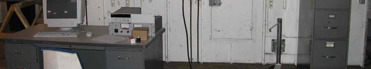
18 Figure 2.3 General Test Site 1 Figure 2.4 General Test Site 2 7

19 2.1 Blower The maximum flow rate requirement of 96 SCFM required a large capacity blower. It was determined that at the maximum flow rate the blower would have to provide a static pressure head of approximately 8 inches of water in order to overcome losses in the system. A Greenheck 3 BISW backward inclined blower was donated for use on this facility. The blower was powered by a Saftronics C1 Vector AC Drive. This variable frequency drive allows for the adjustment of flow rate. The blower was capable of being run with multiple voltages including 46, 23 and 28 volts 3 phase. The voltage available at the location was 28 volts. The adjustment of the VFD frequency setting was done manually by the researcher. 2.2 Nozzle Bank Flow Measurement Standard For this research a nozzle bank chamber was used as the flow measurement standard for comparison with all other volumetric flow measurements in particular comparison with the traversing methods. The nozzle bank was also used for calibration of the flow measurement station (FMS) device. The nozzle bank chamber has three major functions: (1) to connect to and receive flow from the blower, (2) to measure the air flow rate, and (3) to distribute the flow uniformly to the particular duct configuration being used. (Heber et al., 1991) describes the construction of the nozzle chamber. The nozzle chamber was constructed in compliance with AMCA Standard A detailed schematic of the chamber is shown in Figure 2.5 below and pictures are available in Figures 2.9 and 2.1. (Heber et al., 1991) describes the chamber as a baffled multinozzle chamber. The flow chamber consists of five upstream flow diffuser screens, a nozzle bank containing nine nozzles, and three downstream diffuser screens. The chamber was constructed with.75 thick plywood and 1 angle iron framing. (Heber et al., 1991) discusses sealing of the chamber but recommended rechecking of the chamber seals after transportation, which was necessary for this application. Seal tests were performed on the chamber, as well as, on a representative duct configuration. More information about the seal test is given in Appendix A. Diffuser screens are used to distribute and straighten the flow in the nozzle chamber. The diffuser screens are round-wire, square-mesh screens. The location of diffuser screens is based 8

20 on the equivalent diameter (De) of the chamber. These distances are shown in Figure 2.5 below. De is calculated from the inside height and width of the chamber as follows: D 4(width)(height) e (1) (Heber et al., 1991) makes note of the AMCA Standard requirement that the maximum velocity.1de downstream of the diffusers shall not exceed the average velocity by more than 25% when the maximum velocity is more than 2m/s (4 fpm). And that this requirement is not enforced at lower velocities. The nozzle bank consists of nine aluminum-spun nozzles. Their nominal dimensions are available in Table 2.1 and their layout over the duct cross-section is presented in Figure 2.7. A picture of the nozzle bank is available in Figure For the nozzles exact dimensions and uncertainties measured by the researchers see Table 5.1 and Table 5.2. The nozzle bank was used to determine the flow rate. The pressure drop across the nozzle bank was measured by means of two Piezometer rings which detect the static pressure differential. Each ring is made of copper tube and contains four pressure taps, one on each side of the chamber. The static pressure given from each ring represents the average of these four static pressure taps. There is a Piezometer ring on each side of the nozzle bank as well as one in front of the downstream diffuser screens. This third ring was used in Heber s work but was not needed for the current research. The dimensions of the pressure taps are shown in Figure

21 Note: Dimensions in cm Figure 2.5 Nozzle Chamber based on (Heber et al., 1991) 1

22 Note: Dimensions in mm Figure 2.6 Pressure Tap based on (Heber et al., 1991) Note: Dimensions in cm Figure 2.7 Nozzle Layout based on (Heber et al., 1991) 11

23 Table 2.1 Nozzle Dimensions Diameter Area Nozzle Inches cm cm Some alterations to the facility were required for the research. First of all the opening from the chamber to the duct needed to be enlarged. This was due to the large duct test section to be tested. The opening was made significantly larger than the duct and a transition was built to attach the duct to the chamber. The larger transition was implemented to reduce the pressure drop caused by the chamber exit and provide as little disturbance to the exiting flow as possible. A second alteration was made to the opening at the inlet of the chamber to accommodate the new blower. The new 9,6 CFM blower required a larger opening at the chamber entrance. So as not to constrict the flow at the blower exit, the opening in the chamber was made the same size as the blower exit area. Flex duct was used to connect the blower to the chamber. A schematic similar to Figure 2.5 with these changes made is presented in Figure 2.8 below. Pictures of the nozzle chamber are presented in Figure 2.9 and Figure

24 Note: Dimensions in cm Figure 2.8 Altered Nozzle Chamber 13

25 Figure 2.9 Nozzle Chamber 1 Figure 2.1 Nozzle Chamber 2 14

26 Figure 2.11 Nozzle Bank ASHRAE 1245-RP required compliance with ASHRAE standard 12 and the test facility modifications described above were constructed in compliance with AMCA standard It was necessary to show that these nozzle bank chamber modifications were in compliance with both standards. Chamber requirements for each standard are presented in the list below: 1. Pressure Tap Size Dimensions from Figure 2.6 show that we are compliant with both standards. a. ASHRAE standard mm (.59 in) preferred, 3 mm (.118 in) maximum b. AMCA standard 21.6 in (1.52 mm) preferred,.125 in (3.18 mm) maximum c. Current Test Chamber 1. mm (.39 in) 2. Flow Settling Means (Diffusers) Maximum velocity shall not exceed average velocity by more than 25% for velocities greater than 2 m/s (4 fpm). a. ASHRAE standard 12 Requirement at.2 D e downstream of screen b. AMCA standard 21 Requirement at.1 D e downstream of screen 15

27 c. Current Test Chamber Because AMCA standard 21 is the stricter standard we are also compliant with ASHRAE standard 12. Also the average velocity of 349 fpm at 96 cfm in the nozzle chamber is less than 4 fpm. 3. Nozzle Location For both ASHRAE Standard 12 and AMCA 21 the following criteria apply: a. Nozzle centerlines should be at least 1.5 throat diameters away from all chamber walls b. The minimum distance between centers of any two nozzles should be at least 3 throat diameters of the largest nozzle. The modified nozzle bank meets the requirements listed above for both standards. Therefore it represents a suitable means of measuring flow rate for the current ASHRAE RP project and was used as the flow measurement standard for comparison with all other measurements. 2.3 Air Flow Measurement Station (FMS) When measurements were conducted using the diverging tee duct configurations, an additional standard measurement of flow was required. Duct configurations are discussed in detail in section 2.4 Duct Configurations and Fabrication below. The reason for the addition of a second standard was to facilitate accurate measurement of the branch line flow rate. The tee branch line flow rate was determined from the difference between the nozzle bank total flow rate and the FMS flow, with this flow measurement station installed in the main line of the tee. The flow measurement station used for the current project was a Paragon Controls FE 15 Air Flow Measurement Station. Pictures of the FMS are available in Figures 2.12 and 2.13 below. The measurement station has a cross section of 1 x 1. It uses two 9/16 tubes with total and static pressure ports along the tube. The tubes work like Pitot tubes and the average total and static pressures along the tubes are used to determine the dynamic pressure and thus the average velocity. Manufacturers specifications suggest a +/-2% of flow rate accuracy. A separate in-line calibration of the FMS was performed prior to use in the ASHRAE 1245-RP tee testing. The results of the calibration are discussed in section 5.5 Flow Measurement Station Uncertainty. 16

28 Figure 2.12 FMS 1 Figure 2.13 FMS 2 17

29 2.4 Duct Configurations and Fabrication Several duct configurations were used in the current research. All ducts were constructed from #24 gauge galvanized steel in compliance with (SMACNA, 1995). Some of the configurations were used to check equipment and the procedure the researchers planned to use. Other configurations were for the data comparisons needed to achieve the goal of the project. The required lengths of all ducts were determined in the same manner. These lengths depend on the hydraulic diameter of the duct used, or alternately the equivalent diameter. The equivalent diameter was given in Equation (1). All duct lengths associated with ASHRAE 1245-RP were required to be specified in terms of equivalent diameter. D e isn t the traditional hydraulic diameter but rather an equivalent diameter of a circle that has the same area as the duct. The true hydraulic diameter is based on the wetted parameter of the duct. The upstream duct length in each case was at least 2 equivalent diameters. The downstream duct length was always 1 equivalent diameters. Data was collected on several duct configurations. This included various duct sizes, shapes, and the addition of multiple disturbances. Three duct sizes were used upstream of the disturbances. These include 24 z 24, 48 x 12, and 28 x 14. Each upstream duct size had its own set of disturbances and downstream conditions. Table 2.2 contains a summary of the duct configurations along with the duct disturbances to be investigated by ASHRAE 1245-RP. For each duct size, a straight section of duct was needed to evaluate the setup, equipment, instrumentation, and general measurement procedure being used in the research. The duct contained no disturbances and was the length of the appropriate upstream and downstream lengths based on the upstream duct equivalent diameter. Data was collected at the proper locations upstream and downstream of a theoretical disturbance, or in other words the reference plane where the disturbance was to be introduced. The traverses ideally should produce negligible error in the flow measurement at these reference planes because plenty of undisturbed duct length existed upstream and therefore, the flow should be accentually fully-developed at these locations. In addition to the straight duct tests each duct size had multiple disturbances. The 24 x 24 duct had four disturbances; 9 o elbow which included turning vanes and maintained the original duct size, 6 o and 9 o transitions which took the duct from its original 24 x 24 size down to 24 x 12, and a 9 o diverging tee with a 45 o branch entry. The tee also reduced the 18

30 duct size to 24 x 12 in both the main and branch lines. A picture of the tee is available in Figure 2.14 below. The measurements with the tee included three subsets of measurements which varied the branch to common line flow ratio (Qb/Qc). For diverging tees the branch line flow rate (Qb) is measured in the tee s offshoot section of the duct and the common flow rate (Qc) is measured in the upstream section of duct. Data was taken with Qb/Qc ratios of.2,.4, and.6. Figure 2.14 Tee The 48 x 12 and 28 x 14 duct will have the 9 o elbow and 9 o tee configurations but will not have the transitions. Like the 24 x 24 duct, the elbow maintains the size of the upstream duct. The tees have the same downstream duct size for all configurations as well as the same flow ratios Qb/Qc. The 48 x 12 and 28 x 14 duct configurations to be investigated were not part of this thesis. 19

31 Table 2.2 Duct Configurations Upstream Duct Configuration Downsteam Duct Configuration Duct Size D h Duct Length Disturbance Duct Size D h Duct Length Q b / Q c in x in in ft in x in in ft 24 x o Transition 24 x Not applicable 24 x o Transition 24 x Not applicable 24 x o Bend 24 x Not applicable 24 x Tee 24 x ,.4,.6 48 x o Bend 48 x Not applicable 48 x Tee 24 x ,.4,.6 28 x o Bend 28 x Not applicable 28 x Tee 24 x ,.4,.6 Note: Equivalent Diameter D e is defined as D e 4(width)(height) One additional duct configuration was used. Its purpose was to evaluate the leakage in the system. If there is significant leakage from the nozzle bank (where the actual flow rate is computed) to the measurement location it needs to be quantified. The test simply uses the initial 24 x 24 checkout duct setup with the addition of an end cap. This setup ideally yields a theoretical flow rate of SCFM; however, some finite reading was to be expected. The actual leakage flow rate produced was measured at the nozzle bank. A more extensive discussion of the seal testing is given in appendix A. 2

32 CHAPTER 3 - Flow Rate Determination The volumetric air flow rate needed to be determined at the nozzle chamber, duct traverses, and the flow measurement station when a tee disturbance was used. The measurements included air property measurements as well as others depending on the measurement type. For the nozzle chamber and FMS the primary measurement for determining the flow rate was a pressure measurement. For the traverses it was local air velocity measurements. The methods of determining the flow rate as well as a discussion of the air properties required are presented below. Example calculations are available in Appendix E. Much of the data was taken with a Hewlett Packard 3497A Data Acquisition / Switch Unit and computer equipped with LabView software. The LabView software was also used to perform calculations required to determine the flow rate for both the nozzle bank and FMS. The Hewlett Packard 3497A was able to store some data in its output buffer. This was used to do some signal averaging internally and reduce the size of the output file. LabView was able to capture the average of several points from the Hewlett Packard 3497A and store those averages in a text file rather than storing each individual reading. Pictures of the LabView front panels and block diagrams are available in Appendix F. 3.1 Air Properties The primary air properties required for the calculation of volumetric air flow measurement are the air viscosity and density. The air viscosity can be assumed a function of dry bulb temperature only. For ASHRAE 1245-RP the viscosity was calculated with Equation 5 of ASHRAE Standard 12 section 9. The air density can be determined several ways requiring the measurement of one or more air properties including dry bulb temperature, pressure, and humidity. The humidity can be obtained by various methods including the measurement of the wet bulb temperature, relative humidity, or dew point temperature. The simplest way would be to use the ideal gas law and assume the air is dry. The most accurate way to calculate the air density would be to use the dry bulb temperature and pressure along with the humidity measurement. This is the method ASHRAE 1245-RP used. 21

33 The calculation of density including humidity effects is more complicated than the ideal gas assumptions for dry air. It is also more accurate and is therefore recommended for density calculations where high degrees of accuracy are required such as for the nozzle bank used in ASHRAE 1245-RP. The humidity can be determined by measurement of dry bulb temperature along with the measurement of wet bulb temperature, relative humidity, or the dew point temperature. ASHRAE Standard 12 section 9 Equations 1 through 3 use the wet bulb temperature for determining humidity effects on density. If measurements of relative humidity or dew point temperature are used the ASHRAE Fundamentals Handbook or ASHRAE Standard can be used as a reference for density calculations. ASHRAE 1245-RP required ASHRAE Standard 12 as the source for nozzle bank measurements; however, as discussed in section Air density Accuracy Verification other sources can be used for density calculation as long as the maximum error in density doesn t exceed.5%. ASHRAE 1245-RP measured the relative humidity rather than the wet bulb temperature and therefore used the equations of ASHRAE Fundamentals Chapter 6 were used as the source for determining air density for the nozzle bank and FMS. A correction to the density was required for the nozzle bank because the pressure was greater in the chamber than in the general test area. The correction is made with Equation 4 of ASHRAE Standard 12 section 9. The temperature correction isn t required because the temperature is measured in the nozzle chamber rather than the general test area. The individual air properties of barometric pressure, dry bulb temperature, and relative humidity required for the calculation were made with the following instruments. A full listing of instrument specifications is available in Appendix D Barometric Pressure The barometric pressure was recorded with a mercury barometer with a scale readability of.1 hg. Adjustments were made for changes in the density of mercury due to change in temperature Temperature The wet bulb and dry bulb temperatures were measured with a TSI Velocicalc model This wet bulb temperature was used for the 6 o and 9 o transitions on the 24 x 24 upstream duct. The wet bulb temperature wasn t actually measured but calculated internally by the meter from the relative humidity and dry bulb. Standard 12 section 6.9 specifies 22

34 thermometers must have accuracy and scale readability of +/-.5 o C. The Velocicalc unit has an accuracy of +/-.3 o C +.3 o C/ o C for change in instrument temperature from 25 o C and a resolution of.1 o C. After the 6 o and 9 o transitions an Omega 44 series 5, ohm thermistor was implemented. Its measurements were taken continuously with the Hewlett Packard 3497A Data Acquisition / Switch Unit and computer equipped with LabView software. The thermistor has an interchangeability of +/-.2 o C Humidity The relative humidity was first measured before and after each test with the TSI Velocicalc model This was done for the 6 o and 9 o transitions on the 24 x 24 upstream duct. After that a HyCal model IH-362 sensor was used and placed in the flow stream just upstream of the nozzle bank for continuous measurement. Measurements from the HyCal sensor were taken with the Hewlett Packard 3497A Data Acquisition / Switch Unit. The Velocicalc device has an accuracy of +/-3% relative humidity. The accuracy for the HyCal sensor at 25 o C and 5 Vdc excitation is 2.% RH. At the time of this project the humidity sensor was a few years old. Due to this the factory calibration was no longer accurate. A calibrations was performed which resulted in an increase in uncertainty. The calibration was done with a TSI 8347 anemometer; therefore, the uncertainty in the HyCal sensor could be no better than the From the calibration data the random uncertainty in the data and the accuracy of the DVM used in the calibration are shown to be negligible from table 3.1 below. The absolute uncertainty for either the TSI probe or HyCal sensor is given below. Calibrations curves are available in Appendix C. URH 3.% RH Table 3.1 HyCal Humidity Sensor Uncertainty Random TSI 8347 DVM Total Uncertainty Uncertainty Uncertainty Uncertainty % RH % RH Volts %RH % RH

35 3.1.4 Air Density Accuracy Verification Due to the facts that ASHRAE Standard 12 gives a wet bulb temperature specification and our anemometer probe gives relative humidity accuracy it is necessary to show that we are compliant with Standard 12 regardless. Also, it is necessary to show that our use of the ASHRAE Fundamentals method of determining density is compliant with standard 12. The TSI 8347 anemometer uses the procedure of ASHRAE Fundamentals chapter 6 to calculate wet bulb temperature. ASHRAE Fundamentals actually calculates the adiabatic saturation temperature rather than wet bulb temperature but these are very similar. Standard 12 section 9 specifies that other means can be used to calculate density as long as the error in the density calculated does not exceed.5%. Also it can be shown that Equations 11, 28, and 22 from ASHRAE Fundamentals Chapter 6 can be combined to obtain Equation 3 from Standard 12 section 9. The main difference in the calculations is in determining the partial vapor pressure. Table 3.2 shows that by calculating the density using AHRAE Fundamentals or by using ASHRAE standard 12 produces an error or difference between them of much less than.5%. Values of temperature (T), relative humidity (φ), and barometric pressure (P) were varied from a min to max and a value in the middle. Also, Table 3.3 shows that the relative humidity specification of +/- 3% is also sufficient. This table uses 2% relative humidity as an expected value. The table shows that the relative humidity must change by about 5% relative humidity to affect the density for ASHRAE Fundaments by.5%. This would be very similar to the affect on Standard 12 because as table 3.2 showed the densities are very close. The calculations were done over a range of temperatures expected at the data collection site. The barometric pressure used was a typical value measured at the site. Table 3.2 Comparison of Air Density Calculation Ambient Conditions Wet Bulb Air Density kg / m 3 Difference Condition T o C Φ P kpa T* o C ρ ASHRAE ρ std 12 ρ ASHRAE - ρ std 12 min t, min Φ, min P % min t, max Φ, min P % min t, min Φ, max P % min t, max Φ, max P % max t, min Φ, min P % max t, max Φ, min P % max t, min Φ, max P % max t, max Φ, max P % Middle % 24

36 Table 3.3 Relative Humidity Effect on Air Density Ambient Conditions Wet Bulb Air Density Density Change T o C Φ P kpa T* o C ρ ASHRAE kg / m3 ρ new - ρ old % % % % % % % % % Standard Air Density Volumetric air flow measurements for all measurements needed to be based on a standard air density. The correction to standard density is discussed in section 3.5 Correction to Standard Air Density. Standard conditions used are the following: P Standard = Standard Pressure (29.92 inches of mercury) T Standard = Standard Temperature (7 F) 3.2 Nozzle Bank Flow Measurement Standard An ASME nozzle bank was used to determine the standard volumetric air flow rate for comparison with the experimental results obtained from duct traverse methods. The volumetric air flow rate through the ASME nozzle bank was calculated using the method presented in ASHRAE Standard 12. Standard 12 section 9 presents the equations and the procedure for all parameters involved in the determination of flow rate. Measurements taken at the nozzle chamber were used to calculate the flow rate. Some of these include air property measurements discussed in the previous section. Uncertainties of flow rate calculation are discussed in detail in Chapter 5. The volumetric flow rate Q for the chamber can be computed from standard 12 section 9 Equations 16 and 17. (2) m1.414yn 1 P s, 1-2 (CnA n) 25

37 Where Q= Volumetric Flow Rate m = Mass Flow Rate Y n = = Nozzle Expansion Factor 1m Q Air Density in Test Chamber P s, 1-2 = Static Pressure Drop Across Nozzle Bank (3) C n = Discharge Coefficient for Nozzle n A n = Area of Nozzle n These equations can be combined to obtain a single equation for the volumetric flow rate. P Q1414Y (C A ) s, 1-2 n n n The above formulas give the flow in actual units as opposed to standard units, the desired units for the project. The conversion from actual to standard units is discussed in section 3.5 Correction to Standard Air Density. The air density was discussed in section 3.1. The other variables are discussed below. (4) Nozzle Expansion Factor The expansion factor and discharge coefficient are calculated from Standard 12 as well. The expansion factor is a function of Alpha ratio, Beta ratio, and the specific heat ratio and is calculated with Equation 8 of Standard 12 section 9. The Alpha ratio is the ratio of nozzle exit pressure to nozzle approach pressure and is determined with Equation 6 of Standard 12 section 9. The Beta ratio is the ratio of nozzle throat diameter to approach duct diameter and can be assumed for a chamber (ASHRAE Standard 12). The specific heat ratio can be taken as 1.42 (ASHRAE Standard 12). In our case the expansion factor is the same for all nozzles Nozzle Discharge Coefficient In order to compute the discharge coefficient for each nozzle the Reynolds Number must also be calculated. The process of determining the discharge coefficient involves an iterative 26

38 process. An initial estimate of the Reynolds Number must first be computed. The equation for this estimate is similar to the actual version of the equation with some assumptions made. Equation 12 of Standard 12 section 9 is used for the initial estimate. With an initial estimate of the Reynolds Number the iterative process can be performed to obtain the discharge coefficients. Equations 11 and 13 of Standard 12 section 9 are used for the iterative process. Nozzles of different size will have a unique discharge coefficient; therefore, this process including initial estimate of Reynolds Number must be performed for each nozzle of different size. Nozzles with the same diameter will have the same discharge coefficient. In the chamber used there are 9 nozzles available for use; however, there are only 6 unique sizes. It was necessary to determine the number of iterations necessary to converge to an accurate discharge coefficient. Values of Reynolds number and discharge coefficient were calculated for all nozzles with multiple iterations. Temperature and flow rate were adjusted with minimal effect. These adjustments had very little impact on the % change in Cn. The smaller temperatures and smaller flow rates increased the % change slightly but only a couple hundredths of a percent. The percent change from iteration to iteration 1 is barely significant anyway. The second iteration from 1 to 2 is very small and insignificant. The calculations are presented in Table 3.4 showing that a single iteration is sufficient. Table 3.4 Discharge Coefficient Convergence Nozzle Diameter Initial Estimate Iteration 1 Iteration 2 Number inches meters Re Cn Re Cn Change in C n Re Cn Change in C n % % % % % % % % % % % % % % % % % % Static Pressure The pressure drop across the nozzle bank was measured using an Omega PX653 pressure transducer. A power supply was used to supply the pressure transducer with a 24 volt excitation voltage. The output voltage of the pressure transducer was recorded with the Hewlett Packard 3497A Data Acquisition / Switch Unit. 27

39 The static pressure at the nozzle bank inlet was also needed for a pressure correction to the air density discussed in section 3.1 Air Properties. This static pressure at the nozzle bank inlet was measured with different pressure transducers at different points in the project. The transducer voltages were both measured with the Hewlett Packard 3497A Data Acquisition / Switch Unit. The pressure was first measured with the same Omega PX653 pressure transducer as the pressure drop. This device was used for the 6 o and 9 o transitions on the 24 x 24 upstream duct. The pressure was measured before and after each test. After the 6 o and 9 o transitions an additional pressure transducer was purchased to measure nozzle inlet static pressure. The new pressure transducer is a Setra model 264 with the.25% optional accuracy. In order to meet ASHRAE Standard 12 compliance, the pressure must be measured with an accuracy of +/- 1.% of reading. The PX653 and Setra 264 have accuracies based on best fit line (BFL) of.25% full scale output (FSO). It was noticed the pressure transducers didn t quite follow the calibration provided by the manufacturer. A calibration was done following the guidelines in Standard 12 section The description and results of these calibrations are available in appendix C. With a full scale output of 1 W.C. our uncertainty is.25 W.C.. This means that to obtain an accuracy of less than 1.% of reading we must maintain a pressure drop across the nozzles of 2.5 W.C. or larger. 3.3 Air Flow Measurement Station The air flow measurement station (FMS) used was a Paragon Controls FE-15 Air Flow Measurement Station. It was 1 ft square and used pitot probe type pressure measurement for determining the average velocity pressure. It used two horizontal tubes containing holes for capturing the average total pressure and static pressure which can be used to determine the average velocity pressure. The velocity pressure was measured with a Setra 264 similar to that used to measure static pressure drop across the nozzle bank discussed in section Static Pressure. Two transducers were required one with a pressure range of to.5 W.C. and one with a range of to 5 W.C.. The Setra pressure transducers have accuracies based on a best fit line (BFL) of.25% FSO. The velocity pressure can then be converted to a velocity. The air density determined in section 3.1 Air Properties for the general test area is used for determining the velocity from the velocity pressure. It is assumed the temperature and humidity are relatively constant through the duct and that the density at the FMS is significantly close to the density in 28

40 the general test area near the nozzle chamber. The FMS is at about 2 ft from the end of the duct system and the pressure is close to ambient; therefore, the barometric pressure can be used for determining the air density and the density correction for pressure required for the nozzle bank isn t necessary. In theory the averaging in the FMS accurately represents the average velocity pressure in the duct. With this assumption the average velocity would be determined by the following equation: Where V FMS V FMS = Average Velocity at FMS P v = 2P Average Velocity Pressure at FMS o = Air Density in General Test Area The flow rate then can be determined by multiplying the average velocity by the duct area of the FMS. The above discussion is with the assumption the FMS accurately represents the average velocity pressure. It was noticed by ASHRAE 1245-RP that this assumption might not hold for all sizes and aspect ratios of flow measurement stations. A calibration was performed on the FMS used by this project. The calibration uses the following relationships for calculations. Rearranging and substituting gives: Where And C= FMS Flow Coefficient Re = 1 P C V 2 o v (5) ^2 v o FMS (6) odtubev Re FMS o odtube 2P Re v o Co 1 2 (7) (8) C f Re (9) Reynolds Number based on Tube Diameter 29

41 o = Viscosity in General Test Area d tube = Diameter of Tubes inside the FMS In the case of ASHRAE 1245-RP an area ratio is used to help explain some of the reason the FMS was giving readings far off of theoretical. The reduced area due to the tubes in the air stream was on the same order of magnitude as the error in flow rate. The following relationship was established: Where A * 2 C C A ratio (1) FMS Area FMS Area - Tube Area ratio (11) The area ratio is constant and just used to explain the error of the FMS. The calibration resulted in the following relationships for the flow coefficient: 2 * Re Re C e e e An iterative process with Equations 8 and 12 can be used to determine the Reynolds number and flow coefficient. An initial guess of the Reynolds number is determined from the measured velocity pressure at the FMS assuming a flow coefficient of 1. Once the iterations yield significantly small changes in Reynolds number, the final average velocity is obtained by rearranging Equation 7 to solve for V FMS. VFMS Reo odtube (12) (13) 3.4 Flow Measurement by Duct Traverses The traverse measurement of flow rate is simply an average of several velocities in a particular traverse algorithm. At each point in the traverse the local velocity is measured. The number of traverse points is determined by the duct size and algorithm being used. To obtain the flow rate the average velocity must be multiplied by the duct area. For ASHRAE 1245-RP the measurements were done using two probes and two traverse algorithms. 3

42 3.4.1 chebycheff and Algorithms In the case of ASHRAE 1245-RP the traverse algorithms used were log-tchebycheff and equal area. The log-tchebycheff traverse algorithm was obtained from ASHRAE Standard and is also made available in the ASHRAE Fundaments Handbook and (ISO 3966, 1977). The equal area traverse algorithm was obtained from (AABC, 22). A summary of all traverse points for each duct size is available in table 3.5 below. Table 3.5 Traverse Points Duct Size Traverse Algorithm Horizontal Locations Vertical Locations inch x inch (inches) from side of duct (inches) from bottom of duct 24 x x x x 12 Log Tchebycheff Log Tchebycheff Log Tchebycheff Log Tchebycheff 1.8, 6.9, 12, 17.1, , 9.7, 17.6, 24, 3.4, 38.3, , 8.1, 14, 19.9, , 6.9, 12, 17.1, , 6.9, 12, 17.1, , 3.5, 6, 8.5, , 4., 7, 1., 13..9, 3.5, 6, 8.5, , 9, 15, 21 4, 12, 2, 28, 36, , 8.4, 14, 19.6, , 9, 15, 21 3, 9, 15, 21 2, 6, 1 2.3, 7, , 6, Measurement Plane Locations Measurements were taken downstream of the nozzle chamber to simulate balancing tests performed in the field by technicians. The measurements were taken at several locations upstream and downstream of each disturbance. The locations are based on the equivalent diameter of the duct. The equivalent diameter is determined from Equation 1 in Chapter 2. The upstream locations for all duct sizes are 1 and 3 De. The downstream locations for all duct sizes are 1, 2, 3, 5, and 7.5 De. The flow rates measured at these different locations can be compared to the nozzle bank to determine the closest location to the disturbance giving accurate results. Also, corrections can potentially be generated to assist field technicians in obtaining accurate results when measurements have to be taken at an undesirable distance from a disturbance Local Air Velocity Measurements The measurement of air velocity at a specific point in an air stream can be done with several devices. These include rotating vane anemometers, thermal anemometers, pitot-static 31

43 probes, and others. This paper will focus on the two used by ASHRAE 1245-RP, a thermal anemometer and a pitot-static probe Pitot-static Probe Pitot-static probes are used in conjunction with a pressure measurement device measuring the difference between the total pressure and static pressure at each point in the airstream. The pressure measurement device used in ASHRAE 1245-RP was an Alnor EBT 72 electronic balancing tool. Pictures of the pitot-static probe and EBT 72 are available in Figures 3.1 and 3.2 below. The main source of error for this measurement is with the pressure sensor and air property measurement. This is typically provided by the manufacturer, although in many cases a calibration must be performed to insure accurate measurement. The EBT 72 is also a pressure transducer and can measure pressure directly, but was specifically designed with software to be used for air velocity measurement with a pitot-static probe. It also has capability to measure air properties. The device was calibrated for velocity measurement and therefore the manufacturer provides accuracies for velocity measurement. The accuracy of the EBT 72 is +/- 3.% of reading for velocity. Most pressure transducers would only provide accuracies for pressure which would need to be combined with air properties to obtain the uncertainty in velocity. The EBT 72 has the capability to record multiple points and display the average of those points. Recording the average of multiple points reduces the random uncertainty in the measurement which was done for this research. It was necessary to determine how many points to average to significantly reduce the uncertainty without adding too much time to the measurement process. Each point takes about 1 seconds. With lots of points and tests to perform this can add up to a significant increase in measurement time. A test was performed to look into the random uncertainty in the measurement for different numbers of averaged points. Figure 3.3 shows the reduction of random uncertainty for increased number of points recorded. From this plot the researchers decided to record the average of 4 points. This provides a significant reduction in random uncertainty with a manageable amount of time added. 32

44 Figure 3.1 Pitot-static Probe Figure 3.2 EBT 72 Electronic Balancing Tool 33

45 EBT 72 Random Uncertainty Reduction 2.% Random Uncertainty (%) 1.5% 1.%.5%.% Number of Readings Averaged Figure 3.3 EBT 72 Reduction in Random Uncertainty Thermal Anemometer Unlike the pitot-static probe this probe does not measure pressure. Thermal anemometers or hot wire probes use heat transfer to measure air flow. The velocity is related to the convective heat transfer on the probe s wire. The heat transfer is measured from the power input required to keep the wire at a constant temperature. The accuracy of the probe is typically provided by the manufacturer. ASHRAE 1245-RP used a TSI VelociCalc model 8347 air velocity meter. The accuracy of the 8347 is +/- 3.% of reading. A picture of the meter is available in Figure 3.4 below. This anemometer is capable of provided a 1 second average of 1 reading per second so the averaging of multiple points discussed above for the EBT 72 isn t necessary for this device. Figure 3.4 TSI VelociCalc Model 8347 Anemometer 34

46 3.5 Correction to Standard Air Density Volumetric air flow measurements needed to be based on a standard air density. Reporting the results based on a standard density gives the flow rate the air would have been had it been at standard temperature and pressure. This gives an easy way to compare results of various atmospheric conditions. Corrections to the standard air density are made based on the ideal gas law with the equation below. Standard temperature and pressure were defined in section Standard Air Density. PActual T SCFM ACFM Standard P T Standard Actual Where SCFM = Volumetric Air Flow Rate at standard density ACFM = Volumetric Air Flow Rate at actual density P Actual = Actual Pressure T Actual = Actual Temperature This correction must be performed for both the nozzle bank and FMS measurements. The probes used for traversing the ducts can perform this correction internally and don t require a separate correction. The Alnor EBT 72 can perform the correction internally; however, the temperature probe must be used with the EBT 72 in order to accurately make this correction. The TSI VelociCalc model 8347 reports the velocity in standard units (SFPM) with no action or further correction required. (14) 35

47 CHAPTER 4 - Experimental Procedure This chapter describes test procedures for all measurements taken by ASHRAE 1245-RP. These include measurements of air properties, pressures, and velocities. Measurements needed to be taken to determine flow rates in 3 major locations. These include the nozzle chamber, flow measurement station, and traverses. A procedure was also required for accuracy verification of the velocity and pressure probes used. 4.1 Nozzle Chamber Measurement Procedure Some measurements were taken manually before and after each test while others were measured with a Hewlett Packard 3497A Data Acquisition / Switch Unit and computer equipped with LabView software. LabView was also used to calculate all other variables needed to determine the flow rate for the nozzle bank and FMS and print the output to a file. See Chapter 3 for more information on the measured parameters and calculations. The HP 3497A was used to do some averaging. Two LabView files were created, one for setting the flow rate and one for taking the actual data. The reason for the two is that the file for taking actual data can do more averaging while the other can do less averaging but give faster indicator updates. This simply allows for shorter setup times while still providing plenty of averaging for the actual data. The nozzle bank allowed for nozzles to be plugged and therefore raise the pressure drop across the nozzles. Nozzles were plugged with test plugs and/or non-porous inflatable balls. The nozzle pressure drop and inlet static pressure needed to be larger than 2.5 water column in order to achieve desired accuracy in the pressure reading. This was discussed n more detail in Chapter 3. A summary of nominal flow rates used by the project and the nozzles required to be plugged to achieve those flow rates is available in Table

48 Table 4.1 Nozzles Plugged Nominal Flow Rate Nozzles Plugged SCFM Nozzle Number 96 None 72 None , , , 3, 7, , 3, 4, 7, , 3, 4, 7, , 2, 4, 7, 8, , 3, 4, 7, 8, 9 For each traverse at each location a single basic procedure was used. The basic procedure for performing calculations at the nozzle bank is the following: 1. Plug appropriate nozzles. 2. Take all manual measurements required before a test. 3. Run the LabView file for setting the flow rate and adjust fan speed until desired flow rate is achieved. 4. Run the LabView file for actual data collection until the current traverse is complete. Note: equal area traverses were done right after log-tchebycheff but separate files were created. 5. Take all manual measurements required after a test. This basic procedure is consistent throughout the project; however, the procedure may vary some due to changes made by other researchers during the project. This may include implementation of new probes or sensors requiring less manual measurements before and after each test. For example after the 6 and 9 transitions relative humidity and temperature measurements were recorded with LabView and no longer required before and after each test. Also this procedure only includes measurements at the nozzle bank. Other additions to the overall procedure may include adjustments of a damper for tee measurement. 4.2 Flow Measurement Station Procedure Along with the basic procedure additional steps will be included when using the tee disturbance. An additional pressure transducer is used at the end of the main line on the Flow Measurement Station. The specific pressure transducer to use depends on the velocity being measured. Pressure transducers with different ranges were used depending on the velocity being 37

49 measured. This is to insure good uncertainty in the measurement. The appropriate pressure transducer needs to be implemented before the test. In addition to selecting a pressure transducer the Qb/Qc ratio needed to be adjusted. This is done during step 3 above along with the flow rate adjustment. To accomplish this, a damper at the end of the branch line is adjusted. 4.3 Traverse Measurement Procedure The traverse procedure simply involved taking a velocity measurement at each traverse point in Table 3.5. This is done at each location and each velocity. The two probes needed to somehow be positioned at these locations and their accuracies needed to be checked periodically to insure they were working properly. This is discussed below Probe Positioning Procedure A device was built to position the probes in the proper position for the log-tchebycheff and equal area algorithms. Holes could be drilled to insure proper placement along the x axis of the duct. To insure the probes were in the center, a template was used with holes marking the proper log-tchebycheff and equal area horizontal locations. A line was drawn across the duct in the proper location in terms of the number of equivalent diameters up or downstream of the disturbance, the center of the duct was marked, and the templates center was aligned with the center of the duct. To insure proper placement in the vertical direction each probe was equipped with a bracket which allowed it to be screwed into a vertical aluminum column. There was a hole in the column for each point in the log-tchebycheff and equal area traverse patterns. The holes in the column provide proper placement of the probes relative to a center hole on the column. The column with the probe being used then needed to be centered such that the center of the probe was in the center of the duct. To do this the column was placed above the center horizontal location of the duct. A wood dowel with a mark at the duct s nominal center height and 1/8 inch marks on either side of the center mark was used to measure the duct height. The probe was also marked only with 1/16 inch marks. The probe was placed in the center position on the column and adjusted until its center was in the actual center of the duct. The probe was then secured with its bracket. The column was attached to a frame which was positioned on the duct. Figure 4.1 is a schematic of the device using the pitot-static probe and pictures are available in Figures 4.2 and 4.3. A different column needed to be constructed for each vertical duct size because the log- 38

50 Tchebycheff and equal area holes are different for different sizes of duct. The device could be moved along the duct to each measurement location up and downstream of the disturbance. The column could be swapped for different duct sizes. At each measurement location holes were drilled according to the appropriate duct size and x locations summarized in Table 3.5. Figure 4.1 Pitot-static Probe Setup 39

51 Figure 4.2 Pitot-static Probe Picture 1 Figure 4.3 Pitot-static Probe Picture 2 4

52 4.3.2 Probe Specification Compliance Procedure A procedure needed to be implemented to insure that both the thermal anemometer and EBT 72 were working properly. This was done by the use of a water micromanometer. Ideally all three instruments would be used simultaneously and the pitot-static probe would be placed in the same point of the flow stream as the anemometer. Several limitations exist preventing performing this ideal procedure. The probes cannot be in the same spot at the same time because of physical constraints. The probes cannot be tested independently because the anemometer doesn t measure pressure, and therefore cannot be used in conjunction with the micromanometer. Because of these constraints the following describes the procedure used. The pitot-static probe is supported by the usual means with the probe holder setup as in Figure 4.1 above. The probe was placed in the center of the flow stream 3 De upstream of the disturbance. The pitot-static probe was then connected to the EBT 72 in conjunction with the micromanometer and readings of each were taken. Four readings of pressure and velocity were taken and averaged. The pitot-static probe was then removed. In order to make the transition to the anemometer as fast as possible the probe holder was not moved. The anemometer was placed at 3 De. The anemometer was extended the proper distance to reach the center of the duct and supported by a board spanning the base of the holder and by hand. A 1 second average with the anemometer was then taken. There is a schematic of the pitot-static probe setup in Figure 4.1 above and a schematic of the anemometer being used in Figure 4.4 below. Other than for this specification test, when a traverse with the anemometer was conducted the anemometer would be supported by the column rather than the board. 41

53 Figure 4.4 Anemometer Setup This procedure was conducted each time a new duct configuration was built or within no less than a week of a test. Table 4.2 shows the dates of these tests. If each probe's measurements fell within their accuracy specifications, the probes were working properly. If, however, they fell outside of that range further investigation needed to be done. This may include doing the procedure over or a more elaborate calibration check. The procedure was conducted at two velocities for each probe. The velocity wasn t exactly the same on each test but was kept approximately the same by setting the VFD the same. A summary of when these checks were conducted while this researcher was in charge of conducting tests is presented below in. 42

54 Table 4.2 Probe Specification Checks (Passed) Date EBT 72 VFD Settings VelociCalc 8347(A) VFD Settings 6/26/ /14/ /2/ /27/ /26/ /31/ /7/ /14/ /3/ /8/ /19/ /2/ /11/ /19/ /31/ /7/ /15/ /23/ /8/ /27/ /9/ /16/

55 CHAPTER 5 - Experimental Uncertainty Chapter 3 identified the methods for measuring the air flow rate used in ASHRAE RP. A nozzle bank was selected as the standard to base all measurement comparisons on. The nozzle bank was selected for its low uncertainty, large flow range capability, and ease of use with a data acquisition system. A Flow Measurement Station was used as a second standard when there are multiple paths for air to flow. Duct traverses were used for air flow measurements in the duct. The uncertainties in these three measurement types must be determined to form a valid basis of comparison between the measurements which depend on the instruments used to make the measurements. A full listing of instrument specifications is available in Appendix D. Along with the accuracies and precision of all measurements being taken a sensitivity analysis combined with the root mean square method was performed on all calculations. The analysis was performed in the following manner, assuming a generic equation of the following form: Α f B, C (15) Where A, B, and C represent the variables being analyzed and could be anything. There could be more or fewer variables. From a sensitivity analysis the absolute error in the variable A is: Α Α E E E B C Α B C The uncertainty in A is determined from the root mean square method Α Α 2 UΑ UB UC B C This type of analysis was used on all calculations where a sensitivity analysis was required to determine the propagation of errors through the equations. The uncertainties for the calculations discussed in Chapter 3 are presented below. (16) (17) 44

56 5.1 Air Property Uncertainties As discussed in chapter 3 the primary air properties required for the calculation of volumetric air flow measurement are the air viscosity and density. The uncertainties in these two parameters are influenced by the other properties measured to obtain them. The methods by which these other properties are measured greatly affect their uncertainties. The air viscosity can be assumed a function of dry bulb temperature only; therefore, the uncertainty is directly related to the uncertainty in the dry bulb temperature measurement. The air density can be determined several ways requiring the measurement of one or more air properties including dry bulb temperature, pressure, and humidity. The humidity can be obtained by various methods including the measurement of the wet bulb temperature, relative humidity, or dew point temperature. For this project the density is a function of the following variables from ASHRAE Fundamentals. Where P = Barometric Pressure P w = Partial Vapor Pressure T = Dry Bulb Temperature R da = Gas Constant for Dry Air And from a sensitivity analysis the uncertainty in density is: f P, P w, T, Rda (18) 1 P P T Rda w da U U P P U U U w T R The gas constant can be assumed to have negligible error. The accuracy of the pressure and temperature measurement was discussed in chapter 3 section 1. From the ASHRAE Fundamentals Handbook the partial vapor pressure is a function of the following variables. Where = Relative Humidity P ws(t) = Saturation Pressure P, P (T) (19) w f ws (2) 45

57 And the uncertainty is the following: Pw Pw P w P ws(t) P ws(t) U U U The accuracy of the relative humidity measurement was discussed in chapter 3 section 1 and the saturation pressure is a function of temperature only and a sensitivity analysis can be used to determine the effect of temperature on it. (21) 5.2 Nozzle Bank Flow Uncertainty The calculation of volumetric air flow rate through a nozzle bank can be determined using ASHRAE Standard 12 or a similar AMCA standard such as AMCA Standard For ASHRAE 1245-RP ASHRAE Standard 12 was chosen as the standard for volumetric flow rate through a nozzle bank. Calculations of the flow rate taken from this standard are discussed in chapter 3. The following discusses the uncertainties associated with those calculations. The flow rate is a function of the following variables from Equation 3 in chapter 3. n s, 1-2 n n Q f Y, P,, C, A (22) From the sensitivity analysis the following equation for the absolute uncertainty in flow rate is obtained. U Q Q Q Q UY U n P U Y s, 1-2 n P s, 1-2 N 2 2 Q Q UC U n A C n n 1 n A n In order to further analyze the flow rate uncertainty the absolute uncertainty for each variable must also be analyzed. Each one will also have its own independent variables which must be analyzed until we get down to the measured variables discussed in chapter 3. The uncertainty in the air density was discussed in section 5.1. The accuracy of the static pressure drop across the nozzles was discussed in chapter 3. The other uncertainties are evaluated below. (23) Nozzle Expansion Factor Uncertainty The expansion factor is a function of the following three variables discussed in chapter 3. 46

58 Where = = = Alpha Ratio Beta Ratio Specific Heat Ratio n Y f,, (24) In this case the uncertainties of the other variables aren t necessary. The relative uncertainty in the expansion factor is determined by the following equation from (ASME MFC 3M, 1989). Where P s1 = Static Pressure at Nozzle Inlet 2P s, 1-2 Y % (25) n Ps Discharge Coefficient Uncertainty An appropriate uncertainty in the discharge coefficient isn t clear from ASHRAE Standard 12. Other sources were looked at as a reference for an appropriate discharge coefficient uncertainty. These include (AMCA Standard 21, 1985), (ASME MFC 3M, 1989), and (ISO 5168, 1978) none of which resulted in a definite conclusion. AMCA Standard references a tolerance of 1.2% for the discharge coefficients used in that standard. The curve fit equations used in this standard are not the same as ASHRAE Standard 12 so this isn t necessarily appropriate the discharge coefficient used in this research; However, it seems reasonable that the discharge coefficient equations of ASHRAE Standard 12 would have a similar uncertainty. One other standard is being looked into which might discuss the uncertainty of the discharge coefficient used in ASHRAE Standard 12. This is ISO Standard Nozzle Area Uncertainty The nozzle areas are calculated using the nozzle diameter. The uncertainty depends on the nozzle diameter measurement uncertainty. Measurements of all nozzle diameters in the nozzle bank were taken to verify their nominal values and determine the uncertainties in the dimensions. The nominal dimensions were used in calculations of flow rate at the nozzle bank. The measurements were taken from three plains at equal angles apart inside the nozzles. The first 47

59 was vertical. The following two were at 6 o angles in opposite directions from the first. Three readings were taken at each plain. The measurements are presented in Table 5.1. Table 5.1 Nozzle Diameter Measurements Nozzle Number Position Vertical Rotated 6 o Clockwise Rotated 6 o Counter Clockwise Standard deviations and uncertainties were determined from the measurements of each nozzle. Table 5.2 summarizes these uncertainties. The uncertainties in the diameter measurements varied from.22% to a maximum of.64%. Therefore, an uncertainty of.64% in nozzle diameter was used for all nozzles. This is to simplify calculations of uncertainty while using a conservative uncertainty estimate. Table 5.2 Nozzle Diameter Uncertainty Nozzle Number Nominal Dimension Average Standard Deviation t-value Uncertainty inches 2.4E E E E-2 1.2E E E E E-2 Uncertainty m 5.17E E E E-4 2.6E E E E E-4 Uncertainty %.41%.47%.32%.56%.64%.24%.36%.33%.22% Max Uncertainty.64% 5.4 Traversing Algorithm Uncertainties The flow rate of a traverse is discussed in chapter 3 section 3.4. There is an uncertainty associated with the average velocity, duct area, and methods by which the traverse is performed. The first two of these (average velocity and duct area) can be obtained from a sensitivity analysis. The combination of these uncertainties yields the following equation for the uncertainty in the traverse: 48

60 Where M 2 QTraverse Q Traverse 2 Q Traverse A duct V n Traverse A duct V U U U U n 1 n Q Traverse = Volumetric Flow Rate of Traverse A duct = Nominal Area of Duct V n = M = Local velocity at point n Number of Traverse Points U Traverse = Uncertainty in Traverse Methods The constant M depends on the traverse algorithm being used. For ASHRAE 1245-RP this was either log-tchebycheff or equal area. M also depends on the duct dimensions. chebycheff and equal area traverse algorithms are available in ASHRAE Standard and the ASHRAE Fundamentals Handbook. Equal area algorithms are also available in (AABC, 22). The uncertainty in the local velocity measurement of each point in the traverse depends on the method that velocity is measured. Local velocity measurements were discussed in chapter 3 and +/-3% of reading can be obtained for probes used in this project. The uncertainty in the duct area and traverse methods must be discussed in more detail. (26) Duct Area Uncertainty The uncertainty in the area of the duct can have a much larger impact on the uncertainty of the flow rate than may be first realized. The uncertainty in the duct area is affected by the tolerance on duct manufacturing. The nominal area of the duct is calculated with the nominal height and width of the duct. An estimate of the uncertainty can then be obtained assuming the angles of the rectangular duct are at 9 o. Additional error could be present due to variations in duct shape including duct bowing and leaning. The uncertainty in duct area is the following with the assumption that it is a function of the duct dimensions only A 2 duct A duct A Width Height U U U duct Width Height (27) 49

61 With a typical duct dimension tolerance of.25 inches and 2 ft x 1 ft duct dimensions it can quickly be seen that this uncertainty can be as high as 2% or more Traverse Methods Many things can affect the uncertainty in the traverse method. It s largely dependent on the methods used to perform the traverse. As an example this paper will look at uncertainty effects in the methods used by ASHRAE 1245-RP. Many of these would be present in most methods; however, the value of the uncertainty could vary. Things that could affect the uncertainty include but are not limited to the following: Probe Positioning Longitudinal Placement Vertical Placement Probe Tilt Probe Twist Duct Dimensions Duct Shape Assumptions must be made in order to determine this uncertainty. Appropriate assumptions were still being looked into at the submittal of this thesis. 5.5 Flow Measurement Station Uncertainty Air flow measurement stations typically will have an uncertainty specification provided by the manufacturer; however, the device may not have been tested for all variations of the device sold. For example the flow measurement station used by ASHRAE 1245-RP was a 1 ft x 1 ft device which was not tested by the manufacturer. The manufacturer had tested other sizes of flow measurement stations. With accuracy verification test performed by the researchers of ASHRAE 1245-RP it was determined that the device required a calibration. When compared to the nozzle bank the FMS was far outside the 2% of air flow manufacturer spec. The uncertainty of the device should be determined based on this new calibration. The calibration was discussed in chapter 3. The uncertainty is a function of the FMS duct area and the average velocity through the duct. 5

62 Where Q 2 FMS QFMS Q FMS VFMS A V duct FMS Aduct U U U Q FMS = Flow Rate through FMS The uncertainty analysis for the average velocity is slightly more complicated because the flow coefficient and Re depend on each other. A sensitivity analysis was performed to obtain the uncertainty in FMS flow rate. The absolute uncertainty in the average velocity at the FMS is obtained from a sensitivity analysis on Equation 12 of chapter VFMS VFMS VFMS V FMS V FMS Re o o d Re tube o o dtube U U U U U The absolute error in the Re is determined from Equation 6 of chapter 3. Re Re Re Re Re E E E E E E Re Pv C o o d P tube v C o o dtube From Equation 11 of chapter 3 the error in the flow coefficient is dependent on the Re and the random error associated with the calibration and is the following: C E E E Re C Re Rand Combining these equations gives a final error and uncertainty in the Re of the following: 1 Re Re Re Re Re E E E E E E Re C 1 C Pv o o dtube C Re * Re Rand Pv o o dtube URe Re Re Re URand UP U C P v o 1 v o * Re C Re Re C Re U U o d tube o d tube The random uncertainty in the flow coefficient depends on the standard deviation of the data collected in the calibration. The calibration of ASHRAE 1245-RP resulted in the curve fit in Figure 5.1 and deviations of the flow coefficient C* in Figure 5.2. (28) (29) (3) (31) (32) (33) 51

63 FMS Calibration C* C* = -.136(Re/1^3 ) (Re/1^3 ) Re / 1^3 Figure 5.1 FMS Flow Coefficient Calibration Curve FMS Deviation Plot Deviation C* Re / 1^3 Figure 5.2 FMS Calibration Coefficient Deviation Plot These deviations resulted in the following random uncertainty in the flow coefficient C*. URand.2 Because the area ratio used in Equation 9 of chapter 3 is a constant and does not change, the random uncertainty in C and C* are the same. 52

64 CHAPTER 6 - Experimental Data and Analysis This thesis analyzes data collected for the 24 x 24 duct. This includes the disturbances 6 o transition, 9 o transition, 9 o elbow, and 9 o diverging tee. In addition to this there were measurements taken in a straight section of duct with no disturbance, used to show that the system is working properly and to have a basis to compare all other data to. The velocities to be tested were specified in the downstream duct to be 6, 12, 18, and 24 fpm with the exception of the tee measurements. The velocities for the tee were to be the same only specified to be in the upstream duct. This is because if specified to be in the downstream duct the highest velocity with the lowest branch to common line flow ratio would produce a very large and unobtainable flow rate. The purpose of the analysis is to make some comparisons and determine if there are significant changes between them for which conclusions could be drawn. The comparisons made are the following: Measurement Location: Distance from the Disturbance Traverse Algorithm: chebycheff and Measurement Probe: Pitot-static Probe and Anemometer The comparisons made will be between the traverse data for each case and the flow measurement standard. For non-tee measurements this is the nozzle bank. For the tee measurements this is the nozzle bank along with the flow measurement station. The duct traverses represent an idealization of the measurements that technicians would take in the field. It is desired to quantify the error in the traverse measurements. Error is defined as a comparison of the traverse flow rate and the actual flow rate or standard, and is defined as: For tees the standard is defined as: Q SCFM (Traverse) Q SCFM (Standard) Error 1% Q SCFM (Standard) (34) Q SCFM (Standard) Q SCFM (Nozzle Bank) Q SCFM (FMS) (35) For all other measurements it is defined as: 53

65 Q (Standard) Q (Nozzle Bank) SCFM SCFM (36) The traverse data was collected on data sheets, hard copies later transferred to a computer for analysis. The data sheets contain all relevant information including log-tchebycheff and equal area traverse velocities, barometric pressure, VFD setting, number of nozzles plugged and others. Some changes in what parameters were collected were made over the course of the project due to slight improvements in the procedure. For example after the 6 and 9 transitions an additional pressure transducer was purchased and nozzle inlet pressure no longer needed to be recorded before and after each test. The sheets also contain information describing which test the sheet pertains to for organization and file maintenance purposes. An example of a data sheet for the 9 o Elbow is presented in Figures 6.1 and Figure 6.2 below. Measurement Data Tester Craig Date 4/12/27 Location # Diameters 1 Upstream / Downstream Upstream Duct Size 2 x 2 Disturbance 9 o Elbow Intended Flow Rate ( SCFM ) 96 Mean Velocity (SFPM) 24 Anemometer / Pitot Anemometer Figure o Elbow Data Sheet page 1 54

66 Initial Conditions Barometric Pressure "hg 29.9 Frequency hz 52.2 Barometer Temperature o C 75. Nozzles Plugged None Barometric Pressure kpa 98.9 chebycheff Final Conditions Barometric Pressure "hg 29.8 Barometer Temperature o C 75. Barometric Pressure kpa 98.5 Figure o Elbow Data Sheet page 2 The flow rates for the nozzle bank and FMS were calculated with LabView software and printed to a file. Once all the traverse, FMS, and nozzle bank measurements had been made the comparison process began. The error previously mention was calculated for all duct sizes, duct disturbances, duct location, traverse algorithm, velocity, and probe combinations. The results of the calculation of error are presented in plots comparing the error at each location upstream and downstream of the disturbance. There is a plot for each velocity for a total of 4 plots for each duct size and disturbance combination. Results for both probes as well as log-tchebycheff and equal area traverse data are presented in the same plot. Appendix B contains these plots along with summary tables for all duct configurations taken up to the submission of this thesis. An example of the summary and plot is in Figure 6.3 below. 6.1 No Disturbance (Straight Duct) Analysis The duct with no disturbance had 2 De of upstream duct length and 1 De of downstream duct length and should produce fully developed turbulent flow. Measurements should be scattered around an error of within the uncertainty of the measurements. The 55

67 assumption of fully developed flow is confirmed from Figures 6.3 and 6.4 below. Measurement profiles at 3 De upstream and 7.5 De downstream of the theoretical disturbance, had there been one, are shown. It appears from the plots that the flow profile isn t changed very much between the locations and the flow profile is fairly symmetrical, although they appear to be slightly skewed. This suggests that the flow is fully developed or close to it. Horizontal Profile 96 SCFM Velocity (fpm) Position (inches) Vertical Profile 96 SCFM Velocity (fpm) Position (inches) Figure 6.3 Velocity Profiles 3 De Upstream 56

68 Horizontal Profile 96 SCFM Velocity (fpm) Position (inches) Vertical Profile 96 SCFM Velocity (fpm) Position (inches) Figure 6.4 Velocity Profiles 7.5 De Downstream Based on the discussion in Chapter 5, a 1.6% traverse uncertainty estimate was calculated for the 24 x 24 duct. This is based on the +/-3% accuracy of the probes being primarily random uncertainty with small bias error and a +/-.25 duct dimension tolerance. It doesn t include uncertainty in all aspects of the traverse such as proper probe placement because these are still being investigated. From Figure 6.5 below it appears the two probes are obtaining the same reading within this uncertainty. This suggests that the assumption that the probe accuracy is primarily random uncertainty is appropriate and the bias error of the probes is small. An initial 57

69 estimate of the uncertainty in the nozzle bank was also performed which gave an uncertainty between.75% and 1.75% depending on flow rate. This was based on an assumption of a 1.% uncertainty in the nozzle discharge coefficient with is still under investigation. The error or difference between the traverses and the nozzle bank for the log-tchebycheff measurements appear to be scattered around for all measurement locations and within the uncertainties of the nozzle bank and traverse. This suggests that log-tchebycheff is an accurate measurement technique when a fully developed flow exists. The equal area data errors appear to be higher than the log-tchebycheff errors for both probes. From Figure 6.5 it appears that the differences between the two are about 3 to 4% on average. This is consistent over all measurement locations upstream and downstream of the theoretical disturbance location. Measurement Pitot Probe Anemometer Location Q(Standard) Traverse Error Q(Standard) Traverse Error Q(Standard) Traverse Error Q(Standard) Traverse Error De SCFM SCFM % SCFM SCFM % SCFM SCFM % SCFM SCFM % SFPM Straight Duct Error % " x 24" Duct, No Disturbance, 12 sfpm Measurement Location De Log T - Pitot Probe Equal A - Pitot Probe Log T - Anemometer Equal A - Anemometer Figure 6.5 No Disturbance 12 SFPM Data Example 6.2 Single Flow Path Disturbance Analysis The single flow path disturbances include the 6 o transition, 9 o transition, and 9 o elbow. Examples of data plots for these disturbances are available in Figures 6.6 through 6.8 below. All data for the tests can be reviewed in Appendix B. As in the straight duct, it was noticed that the equal area errors are about 3 to 4% higher on average than the log-tchebycheff 58

70 errors for all three disturbances. Also, it appears there is no significant difference between the probe types for any disturbance. For the 9 o elbow the error differences between measurement locations were consistent and no significant differences are apparent for the effect of measurement location on traverse measurement. For the transitions there appears to be an upward trend in error the further downstream of the disturbance a measurement was taken. This is evident at the 5 De and 7.5 De locations. A possible explanation of this is that for these two locations the traverse plain was at a duct seam. It is believed that boundary layer affects from the seam could possibly have affected the traverse measurements. The reason this trend is apparent on the transition measurements and not the elbow is that the downstream duct size for the transitions is different; therefore, the De and measurement locations are different and the seam is not located so close to a measurement location. The 9 o elbow and straight duct have a 24 x 24 downstream duct and the transitions have a 24 x 12 downstream duct. Measurement Pitot Probe Anemometer Postion Q(Standard) Traverse Error Q(Standard) Traverse Error Q(Standard) Traverse Error Q(Standard) Traverse Error De SCFM SCFM % SCFM SCFM % SCFM SCFM % SCFM SCFM % SFPM 6 o Transition Error % " x 24" Duct, 6 o Transition, 12 sfpm Measurement Location De Log T - Pitot Probe Equal A - Pitot Probe Log T - Anemometer Equal A - Anemometer Figure Transition 12 SFPM Data Example 59

71 Measurement Pitot Probe Anemometer Location Q(Standard) Traverse Error Q(Standard) Traverse Error Q(Standard) Traverse Error Q(Standard) Traverse Error De SCFM SCFM % SCFM SCFM % SCFM SCFM % SCFM SCFM % SFPM 9 o Transition Error % " x 24" Duct, 9 o Transition, 12 sfpm Measurement Location De Log T - Pitot Probe Equal A - Pitot Probe Log T - Anemometer Equal A - Anemometer Figure Transition 12 SFPM Data Example Measurement Pitot Probe Anemometer Location Q(Standard) Traverse Error Q(Standard) Traverse Error Q(Standard) Traverse Error Q(Standard) Traverse Error De SCFM SCFM % SCFM SCFM % SCFM SCFM % SCFM SCFM % SFPM 9 o Elbow Error % 24" x 24" Duct, 9 o Elbow, 12 sfpm Measurement Location De Log T - Pitot Probe Equal A - Pitot Probe Log T - Anemometer Equal A - Anemometer Figure Elbow 12 SFPM Data Example 6

72 6.3 Multiple Flow Path (Tee) Disturbance Analysis Up to the submittal of this thesis only one multiple flow path disturbance had been tested which was the diverging tee on the 24 x 24 upstream duct. The velocity targets of 6, 12, 18, and 24 fpm are the same as the single flow path measurements; however, for a Qb/Qc ratio of.2 the highest velocity couldn t be achieved because of pressure drop and fan limitations. It was decided by the ASHRAE committee to allow 21 fpm to be used for this measurement instead. The results of the tee measurements are much more unusual than the single path disturbances especially with a lower branch to common line flow ratio. The lowest branch to common line flow ratio (Qb/Qc =.2) produced anomalous results for locations close to the tee exit. Specifically locations of 1 and 2 equivalent diameters from the disturbance were greatly affected. This is believed to be partially due to negative velocity pressure readings due to non-parallel flows and even reverse flows as the air moves into the branch of the tee where the measurements are taken. Of course a negative velocity pressure doesn t make since. These readings simply mean that the static pressure port on the pitot-static probe is experiencing a higher pressure than the stagnation port due to the air swirling. An example of a datasheet containing the negative readings obtained is available in Figures 6.1 and 6.11 below. The anemometer and pitot-static probe are both unidirectional devices and do not account for air swirling or reverse flow back toward the tee. This could also be affecting other measurements with other flow ratios and measurement locations but was most noticeable for the.2 ratio. (Beck et al, 21) discusses errors from pitot-static probe readings when reverse or perpendicular flows are present. Figure 6.9 illustrates the conclusions for the paper where a flow coefficient for the pitot-static probe is defined as in Equations 37 and 38. C = p P (37) U P = P - P (38) stagnation The figure shows that completely reverse flow would be likely to produce a reading of and closer to perpendicular flows would tend to produce the negative readings which appear in the data. static 61

73 C p C p (1mph) C p (8mph) Figure 6.9 Pitot Probe Flow Coefficient Variation In general it is more difficult to draw conclusion from the tee data. It is evident that the tee is creating a significant amount of flow measurement difficulties. Figures 6.12 through 6.14 are examples of data collected for each Qb/Qc ratio. Many errors exceed the limits of the plots but it can be seen from the tables that errors reach levels close to 6%. The remaining data is available in Appendix B. The bias between log-tchebycheff and equal area algorithms as well as consistency between probe types is still present for the majority of the measurements upstream of the disturbance, which indicates that the results are consistent with the single flow path measurements. Measurement Data Tester Lance Basgall Date 5/1/28 Location # Diameters 1 Dh Upstream / Downstream Downstream Duct Size 2 x 1 Disturbance 9 o Tee Intended Flow Rate ( SCFM ) 72 Mean Velocity (SFPM) 72 Anemometer / Pitot Pitot Probe Figure Tee Qb/Qc =.2 Datasheet 1 62

74 Initial Conditions Barometric Pressure "hg 28.4 Qb / Qc.2 Barometer Temperature o F 85 Frequency hz Barometric Pressure kpa 95.7 Nozzles Plugged None chebycheff Final Conditions Barometric Pressure "hg 28.4 Barometer Temperature o F 87 Barometric Pressure kpa Figure Tee Qb/Qc =.2 Datasheet 2 Measurement Pitot Probe Anemometer Location Q(Standard) Traverse Error Q(Standard) Traverse Error Q(Standard) Traverse Error Q(Standard) Traverse Error De SCFM SCFM % SCFM SCFM % SCFM SCFM % SCFM SCFM % SFPM 9 Tee Qb/Qc Error % " x 24" Duct, 9 Tee, Qb/Qc.2, 12 sfpm Measurement Location De Log T - Pitot Probe Equal A - Pitot Probe Log T - Anemometer Equal A - Anemometer Figure Tee Qb/Qc =.2 12 SFPM Data Example 63

75 Measurement Pitot Probe Anemometer Location Q(Standard) Traverse Error Q(Standard) Traverse Error Q(Standard) Traverse Error Q(Standard) Traverse Error De SCFM SCFM % SCFM SCFM % SCFM SCFM % SCFM SCFM % SFPM 9 Tee Qb/Qc Error % " x 24" Duct, 9 Tee, Qb/Qc.4, 12 sfpm Measurement Location De Log T - Pitot Probe Equal A - Pitot Probe Log T - Anemometer Equal A - Anemometer Figure Tee, Qb/Qc =.4, 12 SFPM Data Example Measurement Pitot Probe Anemometer Location Q(Standard) Traverse Error Q(Standard) Traverse Error Q(Standard) Traverse Error Q(Standard) Traverse Error De SCFM SCFM % SCFM SCFM % SCFM SCFM % SCFM SCFM % SFPM 9 Tee Qb/Qc Error % " x 24" Duct, 9 Tee, Qb/Qc.6, 12 sfpm Measurement Location De Log T - Pitot Probe Equal A - Pitot Probe Log T - Anemometer Equal A - Anemometer Figure Tee, Qb/Qc =.6, 12 SFPM Data Example 64

76 CHAPTER 7 - Conclusions This paper described the setup of ASHRAE 1245-RP along with a discussion of the initial results. An experimental facility was setup to construct multiple duct configurations and test their influence on volumetric air flow rate measurements. The purpose was to use the results in developing guidelines for field technicians when making test and balance air flow measurements at various distances from a duct disturbance such as a diverging tee, elbow, or transition. Along with the influence of duct disturbance, comparisons of traverse algorithms and probe type were also performed. A nozzle bank upstream of the duct configurations was used as the flow measurement standard for all tests along with a flow measurement station as a second standard for the tests using a diverging tee as the duct disturbance. It was necessary to conduct calibrations on all pressure transducers used for the nozzle bank pressure drop and flow measurement station. A calibration of the flow measurement station used for tee disturbances was also conducted to establish its flow coefficient. A leakage test was conducted to quantify the potential error from leakage through the duct and nozzle chamber which showed a leakage of.12% for disturbances other than the tee and up to 1.6% for the tee. The 1.6% is significant but believed to be an overestimate and applies to the worst case scenario when the branch to common flow ratio is.2. A straight section of duct was constructed to verify that the entire system was working properly and that a uniform fully developed flow could be produced with minimal error. An uncertainty analysis was done for the nozzle bank flow calculation with initial estimates of.75% to 1.75% depending on flow rate. This is still being investigated to determine the appropriate uncertainty in the nozzle discharge coefficient. An uncertainty estimate of 1.6% was determined for the traverse in a 24 x 24 duct. Two traverse algorithms, log-tchebycheff and equal area, were used to traverse the duct, measure the velocity profile, and determine the average flow rate. A pitot-static probe and hot wire anemometer were used to collect local velocity measurements in the duct using the two traverse algorithms. To make comparisons between the duct configurations, traverse location, 65

77 traverse algorithm, and probe type an error or difference between the traverse and flow standard was calculated. Measurements of velocity profiles were taken for a 24 x 24 duct with a 9 o diverging tee, 9 o Elbow, 6 o and 9 o transitions, and with no disturbance. A flow rate was determined from the traverses and compared to the flow standard. No conclusive difference in error was observed due to probe type for the duct configurations mentioned above. It was noticed that there was a consistent bias of 3 to 4% high when the equal area method was used as the traverse algorithm versus log-tchebycheff. This could be partially due to the fact that the equal area traverse requires fewer local velocity measurements points than log-tchebycheff for the duct sizes tested. More likely this is more significantly due to the fact that the log-tchebycheff method includes points closer to the duct wall than equal area. For the single flow path measurements there was no conclusive difference in observed error due to measurement location. For the diverging tee measurements; however, large anomalous errors were observed especially at locations downstream of the disturbance and close to the tee with low branch to common line flow ratios. Measurements upstream of the disturbance did seem to still produce the bias of 3 to 4% high when equal area is used. Also for upstream measurements, the probes seemed to give consistent readings with respect to each other. Tests conducted up to the submittal of this thesis were comprised of all the 24 x 24 duct disturbances included the diverging tee. The remaining data will be collected and analyzed by other researchers. 66

78 References 1. ANSI/ASHRAE Standard Method of Testing to Determine Flow Resistance of HVAC Ducts and Fittings. American Society of Heating, Refrigeration, and Air- Conditioning Engineers, Inc. 2. ANSI/AMCA Standard Laboratory Methods of Testing Fans for Rating. Air movement and Control Association, Inc. 3. ASHRAE Standard Practices for Measurement, Testing, Adjusting, and Balancing of Building Heating, Ventilation, Air-Conditioning, and Refrigeration Systems. American Society of Heating, Refrigeration, and Air-Conditioning Engineers, Inc. 4. ASHRAE (21). Handbook: Fundamentals. American Society of Heating, Refrigeration, and Air-Conditioning Engineers, Inc. 5. ASME MFC 3M Measurements of Fluid Flow in Pipes Using Orifice, Nozzle, and Venturi. American Society of Mechanical Engineers 6. Bardot, Dawn (2). Determining the Influence of Turbulence Intensity on the Performance of Rotating Vane Anemometers (Thesis, Kansas State University, 2). 7. Heber, A.J., Cole S.E., & Murphy J.P. (1991). Facility for Testing Exhaust Ventilation Fans. Applied Engineering in Agriculture, 7(5), Kaiser, K. J. (1993). Experimental, Analytical, and Numerical Evaluations of Commercial Ceiling and Wall Ventilation Inlets (Thesis, Kansas State University, 1993). 9. ISO Measurement of fluid flow in closed conduits Velocity area method using pitot static tubes. International Organization of Standardization 1. ISO Measurement of Fluid Flow: Estimation of Uncertainty of a flow-rate measurement. International Organization of Standardization 11. ANSI/ASHRAE Standard (RA 92). Standard Methods for Laboratory Airflow Measurement. American Society of Heating, Refrigeration, and Air-Conditioning Engineers, Inc. 67

79 12. ANSI/ASHRAE Standard (RA 26). Standard Method for Measurement of Moist Air Properties. American Society of Heating, Refrigeration, and Air-Conditioning Engineers, Inc. 13. Foltz, D. F. (1984). The Systematic and Random Errors of Portable Air Flow Balancing Instrumentation with Various Ventilation System Fittings. ASHRAE Transactions, 9(2B), George, R., Finaish, F., Sauer, H., and Howell, R. (1994). Predicting the Temperature, Humidity, Pressure, and/or Density Effects on Velocity Instrumentation. ASHRAE Transations, 1(1), Howell, R., Sauer, H., and Lahmon, R. (1984). Experimental K-factors for Finned Tube Coils Using a Rotary Vane Anemometer. ASHRAE Transactions, 9(2B), Howell, R., Sauer, H., and Lahmon, R. (1986). Influence of Upstream Disturbances on Correlation Coefficient for Vane Anemometers at Coil Faces. ASHRAE Transactions, 92(1A), Howell, R. and Sauer, H. (1987). Velocity Variation Effects on a Rotating Vane Anemometer at Coil Faces. ASHRAE Transactions, 93(2), Howell, R. and Sauer, H. (1989). Airflow Measurements at Coil Faces with Vane Anemometers-Experimental Results. ASHRAE Transactions, 95(2), Howell, R. and Sauer, H. (199). Field Measurement of Air Velocity Pitot Traverse of Vane Anemometer. ASHRAE Journal, March 199, 32(3), Howell, R. and Sauer, H. (199). Airflow Measurements at Coil Faces with Vane Anemometers-Statistical Correlation and Recommended Field Measurement Procedure. ASHRAE Transactions, 96(1), Suppo, M. (1984). Airflow Measurement at Air-System Coils Using the Rotating Vane Anemometer. ASHRAE Transactions, 9(2B), Beck, B., Hosni, M., and Morris, D. (2). Determining Influence of Turbulence Intensity on the Performance of Rotating Vane Anemometers. Final Report, ASHRAE Research Project 986-RP. 23. Morris, D., Beck, B., and Hosni, M. (21). Influence of Turbulence Intensity on the Performance of Rotating Vane Anemometers. ASHRAE Transactions, 17(1). 68

80 24. Beck, B., Morris, D., and Hosni, M., Uncertainty Analysis of the Experimental Results Investigating the Effects of Turbulence Intensity on the Performance of Rotating Vane Anemometers. Proceedings of the ASHRAE Summer Symposium, June MacFerren, E. (1999). vs. chebycheff. HPAC Engineering, 71(12), SMACNA. (1995). HVAC Duct Construction Standards. 2nd Edition. 27. Beck, B. Terry, Payne, Greg, and Heitman, Trevor, The Aerodynamics of the Pitot-Static Tube and its Current Role in Non-Ideal Engineering Applications. Paper Number AC , Proceedings of the ASEE 21 Annual Conference & Exposition, Louisville, Kentucky, June 2-23,

81 Appendix A - Seal Test One Assumption in our measurements is that of minimal leakage in the duct or other parts of the system, in particular after the nozzle bank where the true flow rate is measured. Any leakage after the nozzle bank affects the apparent flow rate at the particular measurement location. The amount of leakage should be quantified to determine if it is significant. The seal test was performed early in the project and some issues with standard 12 compliance existed. Also, equations from (AMCA, 1985) were used because that is what the previous thesis using this nozzle chamber (Kaiser, 1993) used and standard 12 was not yet implemented. If, because of this, we assume a large uncertainty on the leakage measured it will still show minimal leakage. The following describes the test performed to determine the severity of leakage the system has. A.1 Duct Sealing Procedure Each situation will use sealant and the same seal procedure. This procedure includes using Kingco super-seal water based duct sealant or equivalent duct sealant. The sealant is applied to all the S Lock and Drives at each seam. The transition from the nozzle chamber to the duct is sealed with weather stripping. A.2 Seal Test Procedure A seal test was conducted on the straight 24 x 24 duct with no disturbances. An end cap, shown in Figure A.1, was placed on the end of the duct to reduce the flow to a theoretical value of SCFM. The flow actually measured gives us a representative measurement of the amount of leakage. The static pressure in the duct was brought to 1 water column. This is a higher pressure than the duct will see in all situations of this research except the tee. A second leakage test needed to performed for the tee and is discussed in section A.4 Leakage Check for Tee. At the maximum flow rate of 96 SCFM the duct maximum duct pressure is approximately.75 based on experimental data. Therefore any leakages produced by this pressure will be larger than the actual leakage during the tests. This pressure was measured at 1 7

82 equivalent diameter upstream of the theoretical disturbance location. The maximum duct pressure mention previously comes from the total static pressure drop in the duct and would be located at the duct entrance. It was determined from an example of experimental data and calculated from the difference between (total static pressure at the nozzle inlet) and the (static pressure drop across the nozzles). Any pressure downstream of the nozzle chamber would be less than that. While maintaining this pressure the leakage rate was measured at the nozzle bank. All nozzles but the smallest were plugged. This was to give higher pressure drop across the nozzle bank and therefore greater accuracy from our pressure transducer. Figure A.1 End Cap A.3 Duct Leakage Measurement The average leakage measured was 11.6 SCFM. This corresponds to the following percentages for each flow rate which can be seen in table A.1. The table is a little misleading in that it shows a possible leakage of close to 1% at the lowest flow rate. This is incorrect because the duct pressure was much higher than it would have been at that actual tested flow rate showing an unrealistic leakage that would not be present. In reality the duct pressure would be less than.1 and the leakage would be quite small. The higher flow rate cases are the ones with 71

83 meaning and even they are a maximum. The most realistic is the closest to the flow rate that would be obtained with 1 duct pressure which is 96 SCFM. At that flow rate the leakage rate is.12%. ASHRAE Standard 12 specifies a maximum leakage of no more than.5%. Even with large uncertainty in our leakage measurement we are significantly below this. This is especially true due to the fact that the duct pressure was significantly larger than expected during the test. The fluctuations in the leakage rate are also shown in Figure A.2. Table A.1 Nozzle Leakage Percentage Nominal Flow Rate SCFM Leagage SCFM % % % % % % % % % % Leakage Flow Rate (SCFM) Time (s) Figure A.2 Leakage Fluctuations 72

84 A.4 Leakage Check for Tee When the tee was installed it was realized that much higher duct pressures would be encountered. It was necessary to quantify the leakage with the higher duct pressure especially with a branch to common flow ratio (Qb/Qc) of.2 and the highest flow rate. Duct pressure could reach over 5 inches of water column. The leakage was in fact higher and additional duct sealant and reinforcement was necessary. Wooden frames were placed around the duct seams to limit warping and sealant cracking. The following duct leakage was obtained after the reinforcements were in place shown in Figure A.3 below. Leakage (SCFM) Duct Leakage Duct Pressure (Inches H2O) Figure A.3 Duct Leakage for Tee At the highest flow rate of 96 SCFM the duct leakage is approximately 15 SCFM or 1.6%. This is at the point greater than 5 H2O and represents the highest leakage expected with Qb/Qc =.2. Not all tee configurations and flow rates will have this high of leakage. This is more significant than the previous measurements without the tee but should be the worst case scenario considering for actual tests the 5 H2O is only at the duct inlet and decreases down the length of the duct. A.5 Seal Test Conclusions The seal tests described above were conducted and determined the leakage rate at 1 W.C. static pressure for all duct disturbances other than the tee and up to 5 W.C. for the tee. 73

85 The leakage without the tee was determined to be small, around.12% at the highest flow rate. This is the percentage from the flow rate where the duct pressure most closely represents values actually seen. This leakage is significantly smaller than the requirement of ASHRAE Standard 12; therefore, the duct seal procedure proves to be adequate for this research. The leakage at a duct pressure seen by the tee was higher caused by increased pressure drop especially when the branch to common flow ratio is small. The leakage could be as high as 1.6% although this is believed to be a worst-case estimate. 74

86 Appendix B - Data B.1 Data (24 x 24 Upstream Duct Size, No Disturbance) Measurement Pitot Probe Anemometer Location Q(Standard) Traverse Error Q(Standard) Traverse Error Q(Standard) Traverse Error Q(Standard) Traverse Error De SCFM SCFM % SCFM SCFM % SCFM SCFM % SCFM SCFM % SFPM Straight Duct Error % " x 24" Duct, No Disturbance, 6 sfpm Measurement Location De Log T - Pitot Probe Equal A - Pitot Probe Log T - Anemometer Equal A - Anemometer Figure B.1 Data - No Disturbance, 6 fpm 75

87 Measurement Pitot Probe Anemometer Location Q(Standard) Traverse Error Q(Standard) Traverse Error Q(Standard) Traverse Error Q(Standard) Traverse Error De SCFM SCFM % SCFM SCFM % SCFM SCFM % SCFM SCFM % SFPM Straight Duct Error % " x 24" Duct, No Disturbance, 12 sfpm Measurement Location De Log T - Pitot Probe Equal A - Pitot Probe Log T - Anemometer Equal A - Anemometer Figure B.2 Data - No Disturbance, 12 fpm Measurement Pitot Probe Anemometer Location Q(Standard) Traverse Error Q(Standard) Traverse Error Q(Standard) Traverse Error Q(Standard) Traverse Error De SCFM SCFM % SCFM SCFM % SCFM SCFM % SCFM SCFM % SFPM Straight Duct Error % 24" x 24" Duct, No Disturbance, 18 sfpm Measurement Location De Log T - Pitot Probe Equal A - Pitot Probe Log T - Anemometer Equal A - Anemometer Figure B.3 Data - No Disturbance, 18 fpm 76

88 Measurement Pitot Probe Anemometer Location Q(Standard) Traverse Error Q(Standard) Traverse Error Q(Standard) Traverse Error Q(Standard) Traverse Error De SCFM SCFM % SCFM SCFM % SCFM SCFM % SCFM SCFM % SFPM Straight Duct Error % 24" x 24" Duct, No Disturbance, 24 sfpm Measurement Location De Log T - Pitot Probe Equal A - Pitot Probe Log T - Anemometer Equal A - Anemometer Figure B.4 Data - No Disturbance, 24 fpm B.2 Data (24 x 24 Upstream Duct Size, 6 Transition) Measurement Pitot Probe Anemometer Location Q(Standard) Traverse Error Q(Standard) Traverse Error Q(Standard) Traverse Error Q(Standard) Traverse Error De SCFM SCFM % SCFM SCFM % SCFM SCFM % SCFM SCFM % SFPM 6 o Transition Error % 24" x 24" Duct, 6 o Transition, 6 sfpm Measurement Location De Log T - Pitot Probe Equal A - Pitot Probe Log T - Anemometer Equal A - Anemometer Figure B.5 Data - 6 Transition, 6 fpm 77

89 Measurement Pitot Probe Anemometer Postion Q(Standard) Traverse Error Q(Standard) Traverse Error Q(Standard) Traverse Error Q(Standard) Traverse Error De SCFM SCFM % SCFM SCFM % SCFM SCFM % SCFM SCFM % SFPM 6 o Transition Error % 24" x 24" Duct, 6 o Transition, 12 sfpm Measurement Location De Log T - Pitot Probe Equal A - Pitot Probe Log T - Anemometer Equal A - Anemometer Figure B.6 Data - 6 Transition, 12 fpm Measurement Pitot Probe Anemometer Location Q(Standard) Traverse Error Q(Standard) Traverse Error Q(Standard) Traverse Error Q(Standard) Traverse Error De SCFM SCFM % SCFM SCFM % SCFM SCFM % SCFM SCFM % SFPM 6 o Transition Error % " x 24" Duct, 6 o Transition, 18 sfpm Measurement Location De Log T - Pitot Probe Equal A - Pitot Probe Log T - Anemometer Equal A - Anemometer Figure B.7 Data - 6 Transition, 18 fpm 78

90 Measurement Pitot Probe Anemometer Location Q(Standard) Traverse Error Q(Standard) Traverse Error Q(Standard) Traverse Error Q(Standard) Traverse Error De SCFM SCFM % SCFM SCFM % SCFM SCFM % SCFM SCFM % SFPM 6 o Transition Error % 24" x 24" Duct, 6 o Transition, 24 sfpm Measurement Location De Log T - Pitot Probe Equal A - Pitot Probe Log T - Anemometer Equal A - Anemometer Figure B.8 Data - 6 Transition, 24 fpm B.3 Data (24 x 24 Upstream Duct Size, 9 Transition) Measurement Pitot Probe Anemometer Location Q(Standard) Traverse Error Q(Standard) Traverse Error Q(Standard) Traverse Error Q(Standard) Traverse Error De SCFM SCFM % SCFM SCFM % SCFM SCFM % SCFM SCFM % SFPM 9 o Transition Error % 24" x 24" Duct, 9 o Transition, 6 sfpm Measurement Location De Log T - Pitot Probe Equal A - Pitot Probe Log T - Anemometer Equal A - Anemometer Figure B.9 Data - 9 Transition, 6 fpm 79

91 Measurement Pitot Probe Anemometer Location Q(Standard) Traverse Error Q(Standard) Traverse Error Q(Standard) Traverse Error Q(Standard) Traverse Error De SCFM SCFM % SCFM SCFM % SCFM SCFM % SCFM SCFM % SFPM 9 o Transition Error % " x 24" Duct, 9 o Transition, 12 sfpm Measurement Location De Log T - Pitot Probe Equal A - Pitot Probe Log T - Anemometer Equal A - Anemometer Figure B.1 Data - 9 Transition, 12 fpm Measurement Pitot Probe Anemometer Location Q(Standard) Traverse Error Q(Standard) Traverse Error Q(Standard) Traverse Error Q(Standard) Traverse Error De SCFM SCFM % SCFM SCFM % SCFM SCFM % SCFM SCFM % SFPM 9 o Transition Error % " x 24" Duct, 9 o Transition, 18 sfpm Measurement Location De Log T - Pitot Probe Equal A - Pitot Probe Log T - Anemometer Equal A - Anemometer Figure B.11 Data - 9 Transition, 18 fpm 8

92 Measurement Pitot Probe Anemometer Location Q(Standard) Traverse Error Q(Standard) Traverse Error Q(Standard) Traverse Error Q(Standard) Traverse Error De SCFM SCFM % SCFM SCFM % SCFM SCFM % SCFM SCFM % SFPM 9 o Transition Error % " x 24" Duct, 9 o Transition, 24 sfpm Measurement Location De Log T - Pitot Probe Equal A - Pitot Probe Log T - Anemometer Equal A - Anemometer Figure B.12 Data - 9 Transition, 24 fpm B.4 Data (24 x 24 Upstream Duct Size, 9 Elbow) Measurement Pitot Probe Anemometer Location Q(Standard) Traverse Error Q(Standard) Traverse Error Q(Standard) Traverse Error Q(Standard) Traverse Error De SCFM SCFM % SCFM SCFM % SCFM SCFM % SCFM SCFM % SFPM 9 o Elbow Error % 24" x 24" Duct, 9 o Elbow, 6 sfpm Measurement Location De Log T - Pitot Probe Equal A - Pitot Probe Log T - Anemometer Equal A - Anemometer Figure B.13 Data - 9 Elbow, 6 fpm 81

93 Measurement Pitot Probe Anemometer Location Q(Standard) Traverse Error Q(Standard) Traverse Error Q(Standard) Traverse Error Q(Standard) Traverse Error De SCFM SCFM % SCFM SCFM % SCFM SCFM % SCFM SCFM % SFPM 9 o Elbow Error % 24" x 24" Duct, 9 o Elbow, 12 sfpm Measurement Location De Log T - Pitot Probe Equal A - Pitot Probe Log T - Anemometer Equal A - Anemometer Figure B.14 Data - 9 Elbow, 12 fpm Measurement Pitot Probe Anemometer Location Q(Standard) Traverse Error Q(Standard) Traverse Error Q(Standard) Traverse Error Q(Standard) Traverse Error De SCFM SCFM % SCFM SCFM % SCFM SCFM % SCFM SCFM % SFPM 9 o Elbow Error % " x 24" Duct, 9 o Elbow, 18 sfpm Measurement Location De Log T - Pitot Probe Equal A - Pitot Probe Log T - Anemometer Equal A - Anemometer Figure B.15 Data - 9 Elbow, 18 fpm 82

94 Measurement Pitot Probe Anemometer Location Q(Standard) Traverse Error Q(Standard) Traverse Error Q(Standard) Traverse Error Q(Standard) Traverse Error De SCFM SCFM % SCFM SCFM % SCFM SCFM % SCFM SCFM % SFPM 9 o Elbow Error % " x 24" Duct, 9 o Elbow, 24 sfpm Measurement Location De Log T - Pitot Probe Equal A - Pitot Probe Log T - Anemometer Equal A - Anemometer Figure B.16 Data - 9 Elbow, 24 fpm B.5 Data (24 x 24 Upstream Duct Size, 9 Tee) An error in the humidity measurement was discovered in some of the tee data after the deconstruction of the duct configuration. There appears to have been a malfunction in the humidity sensor. Negative humidity was recorded for the corrected data indicated in Table B.1 below. The original data in the table had a positive humidity value and was not affected by a humidity sensor malfunction. It is believed that the malfunction was tied to a drop out of the humidity sensor excitation voltage. This inaccurate humidity measurement affects the nozzle bank and FMS flow rates but does not affect the traverse measurements. The affect results in a small error in density calculation. It can be seen from Table 3.3 that it takes a large change in humidity to have a significant impact on density. The data was corrected by recalculating the flow rates at 5% relative humidity resulting in a decreased density and increased flow rate. The correction is on the order of.3% to.4% increased flow rate. Figures B.17 and B.18 show an example of the change in the data. The change is small and not noticeable on the charts. The rest of the data presented below is corrected when appropriate based on Table B.1. The corrected data now has an absolute uncertainty in relative humidity of +/-5% relative humidity. 83

95 Table B.1 Corrected Data Summary 24 SCFM 48 SCFM Measurement Qb / Qc =.2 Qb / Qc =.4 Qb / Qc =.6 Qb / Qc =.2 Qb / Qc =.4 Qb / Qc =.6 Location pitot anem pitot anem pitot anem pitot anem pitot anem pitot anem 3 Original Original Original Original Original Original Original Original Original Original Original Original 1 Original Original Original Corrected Original Original Corrected Original Corrected Original Original Original 1 Corrected Original Corrected Original Corrected Original Corrected Corrected Corrected Corrected Corrected Corrected 2 Corrected Original Corrected Original Corrected Original Corrected Original Corrected Original Corrected Original 3 Corrected Corrected Corrected Corrected Corrected Corrected Corrected Corrected Corrected Corrected Corrected Corrected 5 Corrected Corrected Corrected Corrected Corrected Corrected Corrected Corrected Corrected Corrected Corrected Corrected 7.5 Corrected Corrected Corrected Corrected Corrected Corrected Corrected Corrected Corrected Corrected Corrected Corrected 72 SCFM 96 SCFM Measurement Qb / Qc =.2 Qb / Qc =.4 Qb / Qc =.6 Qb / Qc =.2 Qb / Qc =.4 Qb / Qc =.6 Location pitot anem pitot anem pitot anem pitot anem pitot anem pitot anem 3 Original Original Original Original Original Original Original Original Original Original Original Original 1 Original Original Original Original Original Corrected Original Original Original Original Original Original 1 Corrected Original Corrected Original Corrected Original Corrected Original Corrected Original Corrected Original 2 Corrected Original Corrected Corrected Corrected Corrected Corrected Corrected Corrected Corrected Corrected Corrected 3 Corrected Corrected Corrected Corrected Corrected Corrected Corrected Corrected Corrected Corrected Corrected Corrected 5 Corrected Corrected Corrected Corrected Corrected Corrected Corrected Corrected Corrected Corrected Corrected Corrected 7.5 Corrected Corrected Corrected Corrected Corrected Corrected Corrected Corrected Corrected Corrected Corrected Corrected Original Data - Uncorrected Measurement Pitot Probe Anemometer Location Q(Standard) Traverse Error Q(Standard) Traverse Error Q(Standard) Traverse Error Q(Standard) Traverse Error De SCFM SCFM % SCFM SCFM % SCFM SCFM % SCFM SCFM % SFPM 9 Tee Qb/Qc Corrected Data Measurement Pitot Probe Anemometer Location Q(Standard) Traverse Error Q(Standard) Traverse Error Q(Standard) Traverse Error Q(Standard) Traverse Error De SCFM SCFM % SCFM SCFM % SCFM SCFM % SCFM SCFM % SFPM 9 Tee Qb/Qc Figure B.17 Data Correction Comparison (Data) 84

96 Error % Error % 24" x 24" Duct, 9 Tee, Qb/Qc.2, 6 sfpm Original Data - Uncorrected Measurement Location De Log T - Pitot Probe Equal A - Pitot Probe Log T - Anemometer Equal A - Anemometer 24" x 24" Duct, 9 Tee, Qb/Qc.2, 6 sfpm Corrected Data Measurement Location De Log T - Pitot Probe Equal A - Pitot Probe Log T - Anemometer Equal A - Anemometer Figure B.18 Data Correction Comparison (Charts) Measurement Pitot Probe Anemometer Location Q(Standard) Traverse Error Q(Standard) Traverse Error Q(Standard) Traverse Error Q(Standard) Traverse Error De SCFM SCFM % SCFM SCFM % SCFM SCFM % SCFM SCFM % SFPM 9 Tee Qb/Qc Error % " x 24" Duct, 9 Tee, Qb/Qc.2, 6 sfpm Measurement Location De Log T - Pitot Probe Equal A - Pitot Probe Log T - Anemometer Equal A - Anemometer Figure B.19 Data - 9 Tee, Qb/Qc =.2, 6 fpm 85

97 Measurement Pitot Probe Anemometer Location Q(Standard) Traverse Error Q(Standard) Traverse Error Q(Standard) Traverse Error Q(Standard) Traverse Error De SCFM SCFM % SCFM SCFM % SCFM SCFM % SCFM SCFM % SFPM 9 Tee Qb/Qc Error % " x 24" Duct, 9 Tee, Qb/Qc.2, 12 sfpm Measurement Location De Log T - Pitot Probe Equal A - Pitot Probe Log T - Anemometer Equal A - Anemometer Figure B.2 Data - 9 Tee, Qb/Qc =.2, 12 fpm Measurement Pitot Probe Anemometer Location Q(Standard) Traverse Error Q(Standard) Traverse Error Q(Standard) Traverse Error Q(Standard) Traverse Error De SCFM SCFM % SCFM SCFM % SCFM SCFM % SCFM SCFM % SFPM 9 Tee Qb/Qc Error % " x 24" Duct, 9 Tee, Qb/Qc.2, 18 sfpm Measurement Location De Log T - Pitot Probe Equal A - Pitot Probe Log T - Anemometer Equal A - Anemometer Figure B.21 Data - 9 Tee, Qb/Qc =.2, 18 fpm 86

98 Measurement Pitot Probe Anemometer Location Q(Standard) Traverse Error Q(Standard) Traverse Error Q(Standard) Traverse Error Q(Standard) Traverse Error De SCFM SCFM % SCFM SCFM % SCFM SCFM % SCFM SCFM % SFPM 9 Tee Qb/Qc Error % " x 24" Duct, 9 Tee, Qb/Qc.2, 21 sfpm Measurement Location De Log T - Pitot Probe Equal A - Pitot Probe Log T - Anemometer Equal A - Anemometer Figure B.22 Data - 9 Tee, Qb/Qc =.2, 21 fpm Measurement Pitot Probe Anemometer Location Q(Standard) Traverse Error Q(Standard) Traverse Error Q(Standard) Traverse Error Q(Standard) Traverse Error De SCFM SCFM % SCFM SCFM % SCFM SCFM % SCFM SCFM % SFPM 9 Tee Qb/Qc Error % " x 24" Duct, 9 Tee, Qb/Qc.4, 6 sfpm Measurement Location De Log T - Pitot Probe Equal A - Pitot Probe Log T - Anemometer Equal A - Anemometer Figure B.23 Data - 9 Tee, Qb/Qc =.4, 6 fpm 87

99 Measurement Pitot Probe Anemometer Location Q(Standard) Traverse Error Q(Standard) Traverse Error Q(Standard) Traverse Error Q(Standard) Traverse Error De SCFM SCFM % SCFM SCFM % SCFM SCFM % SCFM SCFM % SFPM 9 Tee Qb/Qc Error % " x 24" Duct, 9 Tee, Qb/Qc.4, 12 sfpm Measurement Location De Log T - Pitot Probe Equal A - Pitot Probe Log T - Anemometer Equal A - Anemometer Figure B.24 Data - 9 Tee, Qb/Qc =.4, 12 fpm Measurement Pitot Probe Anemometer Location Q(Standard) Traverse Error Q(Standard) Traverse Error Q(Standard) Traverse Error Q(Standard) Traverse Error De SCFM SCFM % SCFM SCFM % SCFM SCFM % SCFM SCFM % SFPM 9 Tee Qb/Qc Error % " x 24" Duct, 9 Tee, Qb/Qc.4, 18 sfpm Measurement Location De Log T - Pitot Probe Equal A - Pitot Probe Log T - Anemometer Equal A - Anemometer Figure B.25 Data - 9 Tee, Qb/Qc =.4, 18 fpm 88

100 Measurement Pitot Probe Anemometer Location Q(Standard) Traverse Error Q(Standard) Traverse Error Q(Standard) Traverse Error Q(Standard) Traverse Error De SCFM SCFM % SCFM SCFM % SCFM SCFM % SCFM SCFM % SFPM 9 Tee Qb/Qc Error % " x 24" Duct, 9 Tee, Qb/Qc.4, 24 sfpm Measurement Location De Log T - Pitot Probe Equal A - Pitot Probe Log T - Anemometer Equal A - Anemometer Figure B.26 Data - 9 Tee, Qb/Qc =.4, 24 fpm Measurement Pitot Probe Anemometer Location Q(Standard) Traverse Error Q(Standard) Traverse Error Q(Standard) Traverse Error Q(Standard) Traverse Error De SCFM SCFM % SCFM SCFM % SCFM SCFM % SCFM SCFM % SFPM 9 Tee Qb/Qc Error % " x 24" Duct, 9 Tee, Qb/Qc.6, 6 sfpm Measurement Location De Log T - Pitot Probe Equal A - Pitot Probe Log T - Anemometer Equal A - Anemometer Figure B.27 Data - 9 Tee, Qb/Qc =.6, 6 fpm 89

101 Measurement Pitot Probe Anemometer Location Q(Standard) Traverse Error Q(Standard) Traverse Error Q(Standard) Traverse Error Q(Standard) Traverse Error De SCFM SCFM % SCFM SCFM % SCFM SCFM % SCFM SCFM % SFPM 9 Tee Qb/Qc Error % " x 24" Duct, 9 Tee, Qb/Qc.6, 12 sfpm Measurement Location De Log T - Pitot Probe Equal A - Pitot Probe Log T - Anemometer Equal A - Anemometer Figure B.28 Data - 9 Tee, Qb/Qc =.6, 12 fpm Measurement Pitot Probe Anemometer Location Q(Standard) Traverse Error Q(Standard) Traverse Error Q(Standard) Traverse Error Q(Standard) Traverse Error De SCFM SCFM % SCFM SCFM % SCFM SCFM % SCFM SCFM % SFPM 9 Tee Qb/Qc Error % " x 24" Duct, 9 Tee, Qb/Qc.6, 18 sfpm Measurement Location De Log T - Pitot Probe Equal A - Pitot Probe Log T - Anemometer Equal A - Anemometer Figure B.29 Data - 9 Tee, Qb/Qc =.6, 18 fpm 9

102 Measurement Pitot Probe Anemometer Location Q(Standard) Traverse Error Q(Standard) Traverse Error Q(Standard) Traverse Error Q(Standard) Traverse Error De SCFM SCFM % SCFM SCFM % SCFM SCFM % SCFM SCFM % SFPM 9 Tee Qb/Qc Error % " x 24" Duct, 9 Tee, Qb/Qc.6, 24 sfpm Measurement Location De Log T - Pitot Probe Equal A - Pitot Probe Log T - Anemometer Equal A - Anemometer Figure B.3 Data - 9 Tee, Qb/Qc =.6, 24 fpm 91

103 Appendix C - Calibrations C.1 Pressure Transducer Calibrations Calibrations of the pressure transducers used in 1245-RP were performed with a water micromanometer, digital multi-meter (DMM), and calibrator typically used in calibration of hot wire anemometers. The pressure source for the calibration was created with an air compressor in conjunction with the calibrator. The calibrator uses air flow from the air compressor to create a pressure difference across a nozzle. The calibrator had an air chamber to deliver consistent air flow in an attempt to limit fluctuations for the compressor. The pressure difference was measured with the micromanometer while hooked up in parallel with the pressure transducer. A voltage reading is taken from the pressure transducer with the DMM. Transducers required to be calibrated were used to measure pressures at the nozzle bank and the FMS. These transducers were discussed in sections Static Pressure and 3.3 Air Flow Measurement Station. Data and plots of the calibration curves obtained are shown below. 92

104 C.1.1 Nozzle Chamber Pressure Transducers Manometer DMM "W.C. Voltage Voltage Omega PX653 Calibration 6 o and 9 o Transitions y =.436x R² = Pressure "H2O Deviation Plot - Omega PX653 6 o and 9 o Transitions Deviation "H2O Pressure "H2O Figure C.1 Omega PX653 1 Pressure Transducer Calibration 1 93

105 Manometer DMM "W.C. Voltage Voltage Omega PX653 Calibration y =.458x R² = Deviation Plot - Omega PX Pressure "H2O Deviation "H2O Pressure "H2O Figure C.2 Omega PX653 1 Pressure Transducer Calibration 2 94

106 Manometer DMM "W.C. Voltage Voltage Setra 264 Calibration y =.526x R² = Deviation Plot - Setra Pressure "H2O Deviation "H2O Pressure "H2O Figure C.3 Setra Pressure Transducer Calibration 95

107 C.1.2 FMS Pressure Transducers Manometer DMM "W.C. Voltage Pressure "H2O Omega PX653 5." W.C. Calibration y =.189x x R² = Voltage Deviation Plot - Omega PX653 5." W.C Deviation "H2O Pressure "H2O Figure C.4 Omega PX653 5 Pressure Transducer Calibration 96

108 Manometer DMM "W.C. Voltage Voltage Setra 264.5" W.C. Calibration y = 1.177x R² = Pressure "H2O Deviation "H2O Deviation Plot - Setra 264.5" W.C Pressure "H2O Figure C.5 Setra Pressure Transducer Calibration 97

109 C.2 FMS Calibration FMS Calibration C* C* = -.136(Re/1^3 ) (Re/1^3 ) Re / 1^3 FMS Deviation Plot Deviation C* Re / 1^3 Figure C.6 FMS Calibration 98

110 C.3 Humidity Sensor Calibration Humidity Sensor Calibration y = 3.78x R² =.993 Voltage Relative Humidity Deviation (RH) Deviation Plot Humidity Sensor Realtive Humidity Figure C.7 Humidity Sensor Calibration 99

111 Appendix D - Instrument Specifications Alnor EBT 72 Electronic Balancing Tool Velocity: +/- 3.% of reading TSI VelociCalc Model 8347 Air Velocity Meter Velocity: +/- 3.% of reading Temperature: +/-.3 o C +.3 o C/ o C for change in instrument temperature from 25 o C Relative Humidity: +/-3% Omega PX653 Pressure Transducers Pressure:.25% full scale output (FSO) based on best fit line (BFL) Setra 264 Pressure Transducers Pressure:.25% full scale output (FSO) based on best fit line (BFL) Paragon Controls FE-15 Air Flow Measurement Station Air Flow Rate: +/-2% HyCal Model IH-362 Humidity Sensor Instrument specification Relative Humidity: +/-2% at 25 o C and 5 Vdc excitation voltage Project Calibration Relative Humidity: +/-3% Omega 44 series 5, ohm thermistor Interchangeability: +/-.2 o C Barometer Scale Readability:.1 hg Meriam Micromanometer Model 34FB2 Range 1 H2O Uncertainty +/-.3 H2O 1

112 Appendix E - Example Calculations This appendix contains an example of the calculations used for this research. Two examples are shown. The first example is for data collected at 3 De upstream of the 9 Tee, the pitot-static probe, and log-tchebycheff traverse at 72 SCFM and Qb/Qc =.4. The second example is for 7.5 De downstream of the 9 Tee, the thermal anemometer, and equal area traverse at 72 SCFM and Qb/Qc =.4. Example 1 includes calculations for air properties, the nozzle bank and the upstream log-tchebycheff traverse. Example 2 includes calculations for the FMS and the downstream equal area traverse. E.1 Example Data E.1.1 Example 1 Data The traverse data for example 1 is presented in Figure E.1 below. Multiple points were recorded with the LabView VI and averaged. The example uses one of those points where the following data point was recorded: Temperature inside Nozzle Chamber (t) 27.3 C Barometric Pressure (P) 98.7 kpa Relative Humidity Sensor Voltage for ( ) Volts Omega Pressure Transducer Voltage for ( Ps, 1-2 ) Volts Setra Pressure Transducer Voltage for ( p 1 ) Volts These values are used with the instrument s calibration curves to achieve the pressure and humidity values. Voltage = (E.1) 3.78 Voltage P s, 1-2 = (E.2).458 Voltage P 1 = (E.3)

113 Relative Humidity: =.355 Nozzle Pressure Drop: Ps, 1-2 = 2.74 H2O = Pa Nozzle Inlet Pressure: P 1 = 5.4 H2O = Pa Initial Conditions Barometric Pressure "hg Qb / Qc.4 Barometer Temperature o C 77.6 Frequency hz Barometric Pressure kpa 98.7 Nozzles Plugged none chebycheff Figure E.1 Traverse Data - 9 Tee, 3 De Upstream, Pitot Probe, 18 fpm E.1.2 Example 2 Data Traverse data for example 2 is presented in Figure E.2 below. Air property and nozzle bank calculations won t be repeated for example 2. The procedure for those is the same as example 1 described in E.2 and E.3 below. The following are the results of these calculations as well as other measured data required for the example. Multiple points were recorded with the LabView VI and averaged. The example uses the average of those points where the following data was recorded: Temperature inside Nozzle Chamber (t) C Barometric Pressure (P) kpa Air Viscosity ( o ) 1.811e-5 Pa s Air Density ( o ) kg/m 3 Nozzle Bank Flow Rate ( Q SCFM (Nozzle Bank) ) SCFM Omega 5. Pressure Transducer Voltage for ( P v ) Volts The value of the pressure transducer output is used with the instrument s calibration curve to achieve the dynamic pressure. In this case a quadratic equation was used because it produced lower deviations than a linear curve. 12

114 2 P v = -.189Voltage Voltage (E.4) P v = H2O = Pa Initial Conditions Barometric Pressure "hg Qb / Qc.4 Barometer Temperature o F 62. Frequency hz 44.6 Barometric Pressure kpa Nozzles Plugged None Figure E.2 Traverse Data - 9 Tee, 7.5 De Downstream, Anemometer, 18 fpm E.2 Example Air Property Calculations This air property example is based on data for example 1 presented in E.1.1 above. The viscosity and density are calculated below. E.2.1 Example Air Viscosity Calculation The air viscosity at the nozzle inlet is a function of temperature and can be calculated from ASHRAE Standard 12 section 9 Equation 5. The viscosity at the nozzle inlet is calculated; however, later equations require the viscosity at the nozzle outlet. The viscosity at the inlet can be used because the temperature doesn t drastically change across the nozzle. Also standard l2 allows for the viscosity to be assumed constant over the range of 4 o C to 32 o C. o = 1.853e-5 Pa s o ( t)1 6 (E.5) E.2.2 Example Air Density Calculation The equations for calculating air density come from ASHRAE Fundamentals chapter 6. The method is as follows: 13

115 Step 1: Calculation of Saturation Pressure The saturation pressure P ws(t) is calculated using Equation 6 of chapter 6 as follows: C8 2 3 l n(p ws(t)) C9 C1 T C11 T C12 T C13 ln(t) (E.6) T Where T = t And the constants in Equation (E.6) are given in Table E.1. P ws = Pa = kpa Table E.1 Saturation Pressure Equation Constants C8 C9 C1 C11 C12 C13 Constants E E E E E E+ Step 2: Calculation of Partial Vapor Pressure The partial vapor pressure P w is calculated using the saturation pressure and the relative humidity. P w = kpa P P (T) w ws (E.7) Step 3: Calculation of Humidity Ratio The humidity ratio is calculated from the partial vapor pressure and barometric pressure. P w.62198* P Pw (E.8) =.81 Step 4: Calculation of Specific Volume per mass of dry air The specific volume per mass of dry air is calculated from the humidity ratio, dry bulb temperature, and barometric pressure P. 14

116 =.8844 m 3 /kg ( * ) da * T* R (E.9) P Step 5: Calculation of Air Density The air density o is calculated from the specific volume and the humidity ratio. o = kg/m 3 1 (E.1) o Step 6: Correction to Air Density There is a correction to the air density for temperature and pressure since these could be different in the nozzle chamber than the general test site. The temperature was measured in the nozzle chamber so no correction is required for it. The pressure correction is made with Equation 4 of ASHRAE Standard 12 section 9. 1 = kg/m 3 P1 1P 1 o (E.11) 1P E.3 Example Nozzle Bank Flow Rate Calculations This nozzle bank flow rate calculation example is based on data for example 1 presented in E.1.1 above. The volumetric flow rate through the nozzle chamber is determined with procedure and equations in Chapter 3. = E.3.1 Example Alpha Ratio Calculation Ps, P 1P 1 (E.12) E.3.2 Example Beta Ratio Calculation The beta ratio is the ratio of nozzle throat diameter to the approach duct diameter. For the chamber the beta ratio can be assumed to be zero. 15

117 d/d (E.13). E.3.3 Example Nozzle Expansion Factor Calculation The nozzle expansion factor Y n is a function of alpha ratio, beta ratio, and the specific heat ratio. In this case it is the same for all nozzles. The specific heat ratio may be taken as 1.42 according to ASHRAE Standard 12. Y n = ) / 2/ n 2/ Y ) (E.14) E.3.4 Example Nozzle Discharge Coefficient Calculation A discharge coefficient must be computed for each nozzle; however, some nozzles are the same and will have the same discharge coefficient. The subscript (n) represents the nozzle number 1 through 9. This example will show the procedure for nozzle 1 and report the result for other nozzles. In this case for 72 SCFM, all nozzles are used and none are plugged. An initial estimate of Re must first be computed. The equation for this estimate is similar to the actual version of the equation with some assumptions made. Re d 1 (Initial Guess) = Re 7,9d P d n 1 s, 1-2 (E.15) n With an initial estimate of Re the iterative process with the equation below can be performed to obtain the discharge coefficient for each nozzle ( C ). The nozzle diameters ( d n ) are available in Table 2.1. It was shown in Chapter 3 that one iteration is sufficient. Cn Re d n n 6 1 (E.16) C 1 (Initial Guess) = Re 1.414C d Y n n d n 1 P n s, 1-2 o (E.17) 16

118 Re d 1 (1 st Iteration) = C 1 (1 st Iteration) = C 2 (1 st Iteration) = C 3 (1 st Iteration) =.9844 C 4 (1 st Iteration) =.9823 C 5 (1 st Iteration) = C 6 (1 st Iteration) = C 7 (1 st Iteration) = C 8 (1 st Iteration) = C 9 (1 st Iteration) =.9844 E.3.5 Example Volumetric Air Flow Rate Calculation The volumetric flow rate is determined from Equation 4 of Chapter 3 and the nozzle areas were presented in Table 2.1. P Q1414Y (C A ) s, 1-2 n n n Q = L/s = ACFM A correction must be made to standard density with Equation 14 of Chapter 3. Q SCFM Q SCFM (Nozzle Bank) = SCFM P Q ACFM T (E.18) (E.19) E.4 Example 1 Traverse Flow Rate and Error Calculations E.4.1 Example 1 Traverse Flow Rate Calculation The traverse flow rate is simply calculated from the average of the velocity measurements in the traverse and the duct area which is 4 ft 2 in this case. The EBT 72 has already converted the velocity measurements to standard density. The average velocity of the traverse points in Figure E.1 is the following: V AVG = SFPM Q Traverse = VAVGA duct (E.2) 17

119 Q Traverse = SCFM E.4.2 Example 1 Traverse Error Calculation For the tee, Equations 34 and 35 of Chapter 6 are used to calculate the error in a traverse downstream of the disturbance. In this case Equations 34 and 36 of Chapter 6 are used because the measurement is upstream of the tee before the flow diverges. The data for example 1 and the flow rate calculated in example E.3 is for one of several points measured with LabView. The flow rates of all the points are averaged and the result ( Q the measurement standard. SCFM SCFM Q (Standard) Q (Nozzle Bank) (Standard) ) is used to determine SCFM (E.21) Q SCFM (Standard) = SCFM The measurement standard along with the traverse flow rate determined in E.4.1 is used to determine the error in the traverse. The result is the same as in the data presented in Appendix B Figure B.24. Error = -1.87% Q SCFM (Traverse) Q SCFM (Standard) Error 1% Q SCFM (Standard) (E.22) E.5 Example FMS Calculation This FMS example is based on data for example 2 presented in E.1.2 above. The FMS calculation uses the FMS calibration curve and equations discussed in Chapter 3. The air density is assumed to be the same as the density at the nozzle chamber calculated with Equation (E.1) prior to the pressure correction. The viscosity is assumed to be the same as at the nozzle chamber. The following constants apply to the FMS. d tube = 9/16 =.143 m A ratio = An initial guess of the Reynolds number is determined from the measured velocity pressure at the FMS assuming a flow coefficient (C) of 1 with Equation 8 of Chapter 3. odtube 2P Re v o Co 1 2 (E.23) 18

120 Re (Initial Guess) = The initial guess of the flow coefficient is then determined by Equations 1 and 12 of Chapter 3. * 2 C C A ratio (E.24) 2 * Re Re C e e e (E.25) * C (1 st Iteration) = C (1 st Iteration) = An iterative process with Equations (E.23) and (E.25) are used to determine the final flow coefficient and Reynolds number. Two iterations were used to determine the final Reynolds. Re (1 st Iteration) = * C (2nd Iteration) = 1.18 C (2nd Iteration) = Re (2nd Iteration) = The final Reynolds number is used to determine the average velocity of the FMS. Re V o FMS odtube (E.26) V FMS = m/s = fpm The average velocity along with the nominal area of the FMS of 1 ft 2 can be used to determine the flow rate through the FMS. Q FMS = VFMS FMS Area (E.27) Q FMS = CFM A correction must be made to standard density with Equation 14 of Chapter 3. Q Q SCFM (FMS) = SCFM SCFM P Q ACFM T (E.28) 19

121 E.6 Example 2 Traverse Flow Rate and Error Calculations E.6.1 Example 2 Traverse Flow Rate Calculation The traverse flow rate is simply calculated from the average of the velocity measurements in the traverse and the duct area which is 2 ft 2 in this case. The anemometer has already given the velocity measurements at standard density. The average velocity of the traverse points in Figure E.2 is the following: V AVG = SFPM Q Traverse = SCFM Q Traverse = VAVGA duct (E.29) E.6.2 Example 2 Traverse Error Calculation For the tee, Equations 34 and 35 of Chapter 6 are used to calculate the error in a traverse downstream of the disturbance. The nozzle bank flow rate provided in E.1.2 and the FMS flow rate calculated in section E.5 are used to determine the measurement standard. Q SCFM (Standard) Q SCFM (Nozzle Bank) Q SCFM (FMS) (E.3) Q SCFM (Standard) = SCFM The measurement standard along with the traverse flow rate determined in E.6.1 is used to determine the error in the traverse. The result is close to the data presented in Appendix B Figure B.24. There is a slight difference due to rounding in this example. Error = 2.16% Q SCFM (Traverse) Q SCFM (Standard) Error 1% Q SCFM (Standard) (E.31) 11

122 Appendix F - LabView Files A computer using LabView 7 and Microsoft Windows XP was used in conjunction with the Hewlett Packard 3497A Data Acquisition / Switch Unit to take measurements. Two LabView VIs were used for the project, one for non-tee measurements and one for tee measurements. The reason for the two is that tee VI includes measurements for the FMS and the non-tee does not. Figures F.1 and F.2 show the front panels of the Vis where the user inputs information and can see the output. The white boxes are inputs and the gray shaded boxes are outputs. The user inputs a 1 or for each nozzle to indicate if the nozzle is plugged () or open (1). Figures F.3 and F.4 show the block diagrams for non-tee and tee measurements respectively. The details of the block diagrams are difficult to read because of the large size. The remaining figures separate the block diagrams into quadrants making it easier to see details. 111

123 F.1 LabView Front Panels Figure F.1 LabView Front Panel, Non-Tee Measurements 112

124 Figure F.2 LabView Font Panel, Tee Measurements 113

125 Receive Input Signal F.2 LabView Block Diagrams Measured Data and Calibration Curves Print to File Density Calculations Nozzle Coefficient Calculations Figure F.3 LabView Block Diagram, Non-Tee Measurements 114

126 Receive Input Signal Measured Data and Calibration Curves Print to File FMS Calculations Density Calculations Nozzle Coefficient Calculations Figure F.4 LabView Block Diagram, Tee Measurements 115

127 Figure F.5 LabView Block Diagram for Non-Tee, Upper Left Corner 116

128 Figure F.6 LabView Block Diagram for Non-Tee, Upper Right Corner 117

129 Figure F.7 LabView Block Diagram for Non-Tee, Lower Left Corner 118

130 Figure F.8 LabView Block Diagram for Non-Tee, Lower Right Corner 119

131 Figure F.9 LabView Block Diagram for Tee, Upper Left Corner 12

132 Figure F.1 LabView Block Diagram for Tee, Upper Right Corner 121

133 Figure F.11 LabView Block Diagram for Tee, Lower Left Corner 122

134 Figure F.12 LabView Block Diagram for Tee, Lower Right Corner 123