AGC (Chapter 9 of W&W) 1.0 Introduction

Transcription

1 AGC Chapter 9 of W&W.0 Introduction Synchronou generator repond to loadgeneration imbalance by accelerating or decelerating changing peed. For example, when load increae, generation low down, effectively releaing ome of it inertial energy to compenate for the load increae. Liewie, when load decreae, generation peed up, aborbing the overupply a increaed inertial energy. Becaue load i contantly changing, an unregulated ynchronou generator ha highly variable peed reulting in highly variable ytem frequency, an unacceptable ituation becaue: NERC penaltie for poor-performance CPS Load performance can be frequency-dependent Motor peed without a peed-drive Electric cloc Steam-turbine blade may loe life or fail under frequencie that vary from deign level. Some relay are frequency-dependent: Underfrequency load hedding relay Volt per hertz relay Frequency dip may increae for given lo of generation

2 The fact that frequency change with the loadgeneration imbalance give a good way to regulate the imbalance: ue frequency or frequency deviation a a regulation ignal. A given power ytem will have many generator, o we mut balance load with total generation by appropriately regulating each generator in repone to frequency change. A a reult of how power ytem evolved, the load-frequency control problem i even more complex. Initially, there were many iolated interconnection, each one having the problem of balancing it load with it generation. Gradually, in order to enhance reliability, iolated ytem interconnected to ait one another in emergency ituation when one area had inufficient generation, another area could provide aitance by increaing generation to end power to the needy area via tie line.

3 For many year, each area wa called a control area, and you will till find thi term ued quite a lot in the indutry. For example, on page 348 of W&W, the term i defined a An interconnected ytem within which the load and generation will be controlled a per the rule in Fig The rule of Fig. 9.0 are dicued in more depth in Section 4.0 below. The correct terminology now, however, i balancing authority area, which i formally defined by the North American Electric Reliability Council NERC a []: Balancing authority area: The collection of generation, tranmiion, and load within the metered boundarie of the Balancing Authority. The Balancing Authority maintain loadreource balance within thi area. Thi definition require another definition []: Balancing authority: The reponible entity that integrate reource plan ahead of time, maintain load-interchange-generation balance 3

4 within a Balancing Authority Area, and upport Interconnection frequency in real time. Each balancing authority will have it own AGC. The baic function of AGC are identified in Fig 9. of W&W Fig. a below. Fig. a Figure 9. hould alo provide a local loop feeding bac a turbine peed ignal to the input of the generator. An alternative illutration howing thi local loop i given in Fig. b. 4

5 Fig. b.0 Hitorical View The problem of meauring frequency and net tie deviation, and then redipatching generation to mae appropriate correction in frequency and net deviation wa olved many year ago by engineer at General Electric Company, led by a man named Nathan Cohn. Their olution, which in it baic form i till in place today, i referred to a Automatic Generation Control, or AGC. We will tudy their olution in thi ection of the coure. Dr. Cohn wrote an excellent boo on the ubject []. 5

6 3.0 Overview There are two main function of AGC:.Load-frequency control LFC. LFC mut balance the load via two action: a. Maintain ytem frequency b.maintain cheduled export tie line flow.provide ignal to generator for two reaon: a. Economic dipatch via the real-time maret b.security control via contingency analyi Below, Fig. c, illutrate thee function. Fig. c 6

7 A it name implie, AGC i a control function. There are two main level of control:.primary control.secondary control We will tudy each of thee in what follow. To provide you with ome intuition in regard to the main difference between thee two control level, conider a power ytem that uddenly loe a large generation facility. The potcontingency ytem repone, in term of frequency meaured at variou bue in the power ytem, i hown in Fig. b and c. Thi i undertood in the context of Fig a and d. T, Electromagnetic torque Mechanical energy Electrical energy T m, Mechanical torque from turbine Fig. a 7

8 Fig. b: tranient time frame Fig. c: tranient time frame 8

9 Fig. d: Tranient & pot-tranient time frame The following chart identifie the variou time interval aociated with the above figure. 9

10 Fig. e 4.0 Two area A mentioned in Section.0 above, on page 348 of W&W, the term control area i defined a An interconnected ytem within which the load and generation will be controlled a per the 0

11 rule in Fig The rule of Fig. 9.0 are applied to a two-control area ytem a illutrated in Table and Fig. 3 below. Table ω P net int Load change Reulting econdary control action - - P L + P L P L - P L P L 0 P L P L 0 P L - Increae P gen in ytem Decreae P gen in ytem Increae P gen in ytem Decreae P gen in ytem Control area Control area P net int P L =Load change in area P L =Load change in area Fig. 3 The table hould be viewed with the following thought in mind: The above ytem may be conidered to be compried of one control area of interet let ay # on one ide of the tie line and a ret of the world control area on the other ide. The

12 ret of the world control area may be one control area or many. All value are teady-tate value not tranient following governor action primary control but before AGC action econdary control. Since all value are teady-tate value, frequency change ω i the ame throughout the interconnection i.e., the ame ω i een in area a area. Frequency change ω i poitive above 60 Hz when load decreae and negative below 60 Hz when load increae. Change in net interchange, denoted by P net int, i poitive for flow increae from area to area and negative for flow decreae from area to area. The indication in the load change column can be undertood to be the caue of the governor action primary control which reult in the frequency and tie line change. There are two important point that come from tudying the above table of rule :

13 . AGC correct both tie line deviation and frequency deviation.. The tie line and frequency deviation are corrected by AGC in uch a way o that each control area compenate for it own load change. Thee are core concept underlying AGC. 5.0 Interchange The interconnection of different balancing authority area create the following complexity: Given a teady-tate frequency deviation een throughout an interconnection and therefore a load-generation imbalance, how doe an area now whether the imbalance i caued by it own area load or that of another area load? To anwer the lat quetion, it i neceary to provide ome definition []: Summary of term: My term W&W term My ymbol W&W ymbol Net actual interchange AP ij Net chedule interchange SP ij Interchange deviation ΔP ij Actual export Total actual net interchange AP i P net int Scheduled export Scheduled or deired value SP i P net int ched of interchange Net export deviation ΔP i ΔP net int 3

14 Net actual interchange: The algebraic um of all metered interchange over all interconnection between phyically Adjacent Balancing Authority Area. Net cheduled interchange: The algebraic um of all Interchange Schedule acro a given path or between Balancing Authoritie for a given period or intant in time. Interchange chedule: An agreed-upon Interchange Tranaction ize MW, tart & end time, beginning & ending ramp time & rate, & type required for delivery/receipt of power/ energy between Source & Sin Balancing Authoritie involved in the tranaction. We illutrate net actual interchange & net cheduled interchange in Fig. 4 below. A 00 mw 0 mw A Scheduled 50 mw 30 mw 80 mw A3 00 mw Actual Fig. 4 4

15 The word net i ued with actual and cheduled interchange becaue there may be more than one interconnection between two area. The net actual interchange between area: A to A: AP =0 MW A to A: AP =-0 MW A to A3: AP 3 =30 MW A3 to A: AP 3 =-30 MW A to A3: AP 3 =-80 MW A3 to A: AP 3 =80 MW The net cheduled interchange between area: A to A: SP =00 MW A to A: SP =-00 MW A to A3: SP 3 =50 MW A3 to A: SP 3 =-50 MW A to A3: SP 3 =-00 MW A3 to A: SP 3 =00 MW The interchange deviation between two area i Net Actual Interchange-Net Scheduled Interchange We will define thi a ΔP ij, o: ΔP ij =AP ij -SP ij In our example: Area : ΔP =AP -SP =0-00=0 MW ΔP 3 =AP 3 -SP 3 =30-50=-0 MW Area : ΔP =AP -SP =-0--00=-0 MW ΔP 3 =AP 3 -SP 3 = =0 MW 5

16 Area 3: ΔP 3 =AP 3 -SP 3 = =0 MW ΔP 3 =AP 3 -SP 3 =80-00=-0 MW Some obervation:.the net actual interchange may not be what i cheduled due to loop flow. For example, the balancing authoritie may chedule 50 MW from A to A3 but only 30 MW flow on the A-A3 tie line. The other 0 MW flow through A. Thi i called loop flow or inadvertent flow..we may alo define, for an area i, an actual export, a cheduled export, and a net deviation or net export deviation a: Actual Export: Scheduled Export: Net Deviation: n AP i AP ij j ji n SP i SP ij j ji 3 n P i P ij j ji 4 W&W ue different nomenclature/terminology, p. 347: 6

17 Total actual net interchange denoted a P net int to mean actual export. Scheduled or deired value of interchange denoted a P net int ched to mean cheduled export. ΔP net int to mean net deviation Since an area net deviation i the um of it interchange deviation per eq. 4, and Since each interchange deviation i Net Actual Interchange-Net Scheduled Interchange per eq., we can write P i n P n AP SP ij ij ij ij j j j j ji ji ji ji n AP n SP ij AP SP 5 Thi ay that the net deviation for an area i jut the difference between the actual export and the cheduled export for that area. Summary of term: My term W&W term My ymbol W&W ymbol Net actual interchange AP ij Net chedule interchange SP ij Interchange deviation ΔP ij Actual export Total actual net interchange AP i P net int Scheduled export Scheduled or deired value SP i P net int ched of interchange Net export deviation ΔP i ΔP net int i i 7

18 3. Net deviation i unaffected by loop flow. For example, in Fig. 5a, the right ide ha the ame net deviation a the left ide but how a new et of actual flow between area, due to a change in tranfer path impedance. But ΔP i doen t change. A 50 mw 00 mw 0 mw 30 mw A3 80 mw A 00 mw Scheduled Actual A 50 mw 00 mw 5 mw 5 mw A3 75 mw A 00 mw Scheduled Fig. 5a What affect net deviation i varying load & varying gen, a illutrated in Fig. 5b, where the right ide ha the ame cheduled flow a the left ide but how new net deviation for area A, A. A 50 mw 00 mw 0 mw 30 mw A3 80 mw A 00 mw Scheduled Actual A 50 mw 00 mw 5 mw 35 mw A3 75 mw A 00 mw Actual Scheduled Fig. 5b We ee that the A actual export i 60 MW intead of the cheduled export of 50MW, ΔP =60-50=0MW. Liewie, the A3 actual export i 40 MW intead of the cheduled 50 MW, ΔP 3 =40-50=-0MW. The area A actual export i till the ame a the cheduled export of -00 MW, ΔP = =0MW. Actual 8

19 Concluion: Area A ha corrected for a load increae in Area A3. So we need to ignal Area A generator to bac down and Area A3 generator to increae. Overall concluion: To perform load-frequency control in a power ytem coniting of multiple balancing authoritie, we need to meaure two thing: Steady-tate frequency deviation: to determine whether there i a generation/load imbalance in the overall interconnected ytem. f f 60 6 When Δf>0, it mean the generation in the ytem exceed the load and therefore we hould reduce generation in the area. Net deviation: to determine whether the actual export are the ame a the cheduled export. Pi APi SPi 5 When ΔP i >0, it mean that the actual export exceed the cheduled export, and o the generation in area i hould be reduced. 9

20 The meaurement of thee two thing i typically combined in an overall ignal called the area control error, or ACE. From the above, our firt impule may be to immediately write down the ACE for area i a: ACE i Pi f 7 Alternatively, ACE i Pi 8 But we note problem with eq. 8. Firt, we are adding quantitie that have different unit. Anytime you come acro a relation that add or more unit having different unit, beware. The econd problem i that the magnitude of the two term in eq. 8 may differ dramatically. If we are woring in MW and Hz or rad/ec, then we may ee ΔP i in the 00 of MW wherea we will ee Δf or Δω in the hundredth or at mot tenth of a Hz. The implication i that the control ignal, per eq. 8, will greatly favor the export deviation over the frequency deviation. 0

21 Therefore we need to cale one of them. To do o, we define area i frequency bia a B i. It ha unit of MW/Hz, o that ACEi Pi Bi 9 We will loo cloely at ue of thi equation for control. Before we do that, however, we need to loo at the ytem that we are trying to control and obtain model for each ignificant part. 6.0 Generator model A well-nown relation in power ytem analyi i the wing equation. Thi equation i derived in EE 554 and relate acceleration of a ynchronou machine to imbalance between input mechanical power and output electrical power, according to H d e Pm P e 0e dt 0 Or, ince ω=dδ/dt, we can write 0 a H de Pm Pe 0 e dt where

22 δ e i the machine torque electrical angle by which the rotor lead the ynchronouly rotating reference; P m i mechanical input power in per-unit P e i electrical output power in per-unit H i the inertia contant in Mjoule/MW=ec given by 0m I H S b S b i the machine MVA rating; I i moment of inertia of all machine mae in g-m 0 6 ; ω 0m i the ynchronou rotor peed in mechanical rad/ec ω 0e i the ynchronou rotor peed in electrical rad/ec will alway be 377 in North America. If you have the EE554 text Anderon& Fouad, you will find a eq..8 in that text. Here, to agree with eq. 9.6 in W&W, we need to mae three change.

23 .Put frequency in pu: H de P dt 0 e e d 0e H 0e 0e dt m P d H P m P e dt where ω=ω e /ω 0e. m P e P e Ue a different inertia term: Anderon & Fouad define the angular momentum of the machine a M; we denote it here a M AF where M AF I0m 6a From repeated below, left, we can write I0m HSb H I0m S b 6b 0m Thu we ee that HSb M AF 7 0m 3

24 and olving for H, we obtain: M AF H 0m S 8 b Subtituting into 5 repeated below, left: d M AF H P m P 0 m d e P dt m Pe Sb dt 9 Now where A&F ue the angular momentum M AF, W&W ue a per-unitized angular momentum, according to M AF M m WW 0 Sb 0 Comparion to 8 indicate M WW H Therefore, we have d M P m P e dt where it i undertood from now on that M=M WW. W&W indicate on pg. 33 that the unit of M are watt per radian per econd per econd. 4

25 However, it i typically ued in a form of perunit power over per-unit peed per econd, a we have derived it above, and here it ha unit of econd. In fact, W&W themelve mention thi pg 33 and ue it in per-unit form in all of the ret of their wor in thi text. 3.Ue deviation: Expre each variable in a um of an equilibrium value and a deviation, i.e., Pm Pm 0 Pm Pe Pe 0 Pe e0 t t t e0 Subtitution of the above into reult in d t M Pm 0 Pm Pe 0 Pe dt 3 Simplifying, and noting that at equilibrium, P m0 =P e0, we have 5

26 M d t dt P m P e 4 Equation 4 i eq. 9.6 in your text and i what W&W ue to repreent the dynamic of a ynchronou machine. Becaue we want to derive bloc diagram for our control ytem, we will tranform all timedomain expreion into the Laplace domain. M P m P e 5 where we have aumed ωt=0= Load model The load upplied by a power ytem at any given moment conit of many type of element, including electronic load, heating, cooing, and lighting load, and motor load, with the latter two type of load compriing the larger percentage. Of thee two, it i quite typical that heating, cooing, and lighting load have almot no frequency enitivity, i.e., their power conumption remain contant for variation away from nominal frequency. More dicuion about variou load type i in [3]. 6

27 Motor load, on the other hand, are different. To ee thi, we will focu on only the induction motor which tend to comprie the larget percentage of motor load. Conider the tandard per-phae teady-tate model of an induction motor, a given in Fig. 6. Fig. 6 From thi model, the electric power delivered to the motor can be derived a: P R th R 3V ' th R X ' th X ' 6 where R th +jx th and V th are the Thevenin equivalent impedance and voltage, repectively, looing from the rotor circuit the junction between jx S and R in Fig. 6 left, bac into the tator circuit. 7

28 Recall that induction motor lip i given by m = 7 where ω S i the mechanical ynchronou peed et by the networ frequency and ω m i the mechanical peed of the rotor. Subtituting 7 into 6 we obtain P R th R 3V ' m th R ' X th X ' 8 Quetion: Let aume that the voltage V th and the mechanical peed ω m remain almot contant the almot i becaue there i ome variation in ω m which can be oberved by plotting torque v. peed curve ee note from EE 559. What happen to P a ω S decreae? 8

29 Example: Aume contant mechanical peed ω m of 80 rad/ec. What happen to for a 4-pole machine when frequency decreae from 60 Hz to 59.9 Hz? Then indicate qualitatively what happen to power drawn by the motor under thi ame frequency deviation. Solution: At 60 Hz, the ynchronou peed i given and correponding lip are given by ω S =πf/p/=π60/4/=88.5 rad/ec = /88.5=0.045 where p i the number of pole. At 59.9 Hz, it i given by ω S =π59.9/4/=88.8 rad/ec = /88.8= And o reduction in frequency caue a reduction in lip. From 6, we ee that thi R ' will caue the term to increae, which will caue the overall power expreion to decreae. Concluion: Power drop with frequency. m 9

30 EPRI [4] provide an intereting figure which compare frequency enitivity for motor load with non-motor load, hown below in Fig. 7. Fig. 7 Figure 7 how that motor load reduce about % for every % drop in frequency. If we aume that nonmotor load are unaffected by frequency, a reaonable compoite characteritic might be that total load reduce by % for every % drop in frequency, a indicated by the total load characteritic in Fig. 7. To account for load enitivity to frequency deviation, we will define a parameter D according to 30

31 D pu change pu change in from which we may write: pu change in load in load frequency D 9a 9b If our ytem ha a % decreae in power for every % decreae in frequency, then D=. In determining D baed on 9a, the bae frequency hould be the ytem nominal frequency, in North America, 60 Hz. The bae load hould be the ame a the bae MVA, S b, ued to per-unitize power in the wing equation 4, repeated here for convenience. M d t dt P m P e 4 In 4, P e i the change in electric power out of the ynchronou generator. The change in electric power out of the ynchronou generator will be balanced by any change in net electric demand in the networ, which we will denote a P L and 3

32 the change in load due to frequency deviation, according to 9b. Therefore Pe PL D 30 Pleae note that thi D differ from the D ued in tability tudie to repreent windage & friction. Subtitution of 30 into 4 reult in d t M Pm PL D t dt 3 Taing the Laplace tranform of 3 reult in M Pm PL D 3 where again we have aumed ωt=0=0. Solving 3 for ω, we obtain M M D D P P m P L M D Input P We model 33 a in Fig. 8. m m P P L Tranfer Function L 33 3

33 ΔP m + Σ - M+D Δω ΔP L Fig Turbine prime mover model The mechanical power i provided by the primemover, otherwie nown a the turbine. For nuclear, coal, ga, and combined cycle unit, the prime-mover i a team turbine, and the mechanical power i controlled by a team valve. For hydroelectric machine, the prime mover i a hydro-turbine, and the mechanical power i controlled by the water gate. We deire a turbine model which relate mechanical power control team valve or water gate to mechanical power provided by the turbine. 33

34 Since the mechanical power provided by the turbine i the mechanical power provided to the generator, we can denote it a P m. We will denote the mechanical power control a P V. Reference [5, p. 4-6] provide a brief but ueful dicuion about turbine model and indicate that a general turbine model i a hown in Fig. 9. NEXT 6 PAGES PROVIDE BACKGROUND ON TURBINE MODELING. YOU SHOULD READ THIS ON YOUR OWN. IN LECTURE, WE SKIP TO PAGE

35 35 Fig. 9 K Σ T 4 + ΔP V T 5 3 K Σ + + T 6 5 K Σ + + T 7 7 K Σ + + ΔP M

36 Thi turbine model can be applied to a multi-tage team turbine, a ingle-tage team turbine, or a hydro-turbine. The multi-tage team turbine i a common type of turbine that ue reheating to provide additional power from the ame team, and a a reult i mot often called a reheat turbine. The principle behind a reheat turbine i that the energy of the team i dependent upon two of it attribute: preure and temperature. Thi can be oberved in a very imple way by recalling that wor done by exerting a force F over a ditance d i given by W=F d. Dividing F by Area A and multiplying d by A, we get W=F/A da, and recognizing F/A a preure, P, and da a volume V, we ee that W=P V. Now the only other thing we need to now i that volume V increae with temperature, and we ee quicly that the energy exerted by an amount of team flowing over turbine blade increae with preure and temperature. 36

37 A typical -tage reheat turbine i hown in Fig. 0 where we oberve that the reheater provide increaed temperature to utilize the reduced preure team a econd time in the low preure turbine. 400 PSI 000 F HP Turbine LP Turbine GEN STEAM VALVE Exhaut 600 PSI 600 F REHEATER 500 PSI 000 F Fig 0 Referring once again to Fig. 9, the time contant T 4 repreent the firt tage, often called the team chet. If the turbine i non-reheat, then thi i the only time contant needed, and the deired tranfer function i given by Pm PV T4 34 For multitage turbine, reference [5] tate that The time contant T 5, T 6, and T 7 are aociated with time delay of piping ytem for reheater and cro-over mechanim The coefficient K, K 3, K 5, and K 7 repreent fraction of total 37

38 mechanical power output aociated with very high, high, intermediate, and low preure component, repectively. Reference [5] alo provide ome typical data for team turbine ytem, reproduced in Table below. Nonreheat Singlereheat Doublereheat Table T 4 T 5 T 6 T 7 K K 3 K 5 K

39 Finally, reference [5] addree hydro turbine: In the cae of hydro turbine, the ituation depend on the geometry of the ytem, among other factor. The overall tranfer function of a hydro turbine i given a Tw Pm PV 0.5T where T w i nown a the water time contant. The ignificance of the above tranfer function i that it contain a zero in the complex right-half plane. From a tability viewpoint, thi may caue ome problem ince thi i a non-minimum phae ytem. Uing the model of Figure 6.5 Fig. 9 in our note one identifie the following parameter: T 4 =0, T 5 =T w /, T 6 =T 7 =0, K =-, K 3 =3, K 5 =K 7 =0. Typical value of T w range from.5 to 5 ec. The above ytem i called non-minimum phae becaue it ha a right-half-plane zero and therefore, in frequency-repone Bode plot, we will ee a greater phae contribution at frequencie correponding to the RHP zero. w 39

40 We will be able to illutrate the baic attribute of AGC by uing the model for the implet turbine ytem the nonreheat turbine, with tranfer function given by 34. For convenience, we write thi tranfer function here, together with that of the generator with load frequency enitivity given by 33: Pm PL Pm PL G M D 33 P m Input T 4 P Tranfer Function V T P Input Subtituting 34 into 33 reult in T 4 P V P L V M D We ee in 35 tranfer function providing frequency deviation a a function of: change in team valve etting and change in connected load. The bloc diagram for thi appear a in Fig.. Fig. illutrate the action of the primary peed controller, which we will decribe next. 40

41 ΔP V +T 4 T ΔP m + - Σ ΔP L M+D G Δω Fig. Σ - ΔP V +T 4 T ΔP m + - Σ ΔP L M+D G Δω Equation 36-37: P P G P m m T P T Q V L Fig. Q 4

42 9.0 Primary peed control The primary peed controller i alo referred to a the peed governor. It ha three purpoe:.regulate the peed of the machine..aid in matching ytem MW generation with ytem MW load. 3.Provide a mechanim through which econdary peed control can act. Regulation of peed mean we will control ω. To control ω, we mut regulate the input power to the machine, denoted in Fig. by P V. Thi require having feedbac from ω to P V. We denote thi feedbac a Q, a hown in Fig.. Uing the impler notation of T and G, we can ee from Fig. that Pm PL G 36 and Pm T PV T Q 37 Subtitution of 37 into 36 reult in 4

43 T Q P G L 38 Solving for ω T T Q G PL G Q G PL G P G L T Q G 39 Appendix A of thee note provide an analyi of a mechanical-hydraulic peed governor that wa ued for many year and till i in ome older power plant. Newer plant today ue computer-baed digital controller. But the concept are the ame; we utilize eq. A from App A to illutrate the relation in notation of App A, the circumflex above variable indicate the Laplace domain in thee equation. P V 53 xˆ E ˆ 5 4 A Pˆ C A Here, i the ame a P V. We drop the E notation, and we ignore P C which i the etpoint power output for now, o that xˆ E P V ˆ xˆ 43

44 The firt ind of governor ever deigned provided imple integral feedbac. Thi i obtained from 40 if 4 i et to 0 in Appendix A, thi correpond to diconnecting rod CDE at point E in Fig. A4 and A5 ee eq. Aa. Then we obtain 5 3 P V ˆ 4 The contant in 4 are combined to obtain: P K G ˆ V 4 Comparing 4 to the bloc diagram of Fig., we ee that KG Q 43 Subtitution of 43 into 39 reult in P KG L G T G 44 The bloc diagram for 44 i hown in Fig

45 Σ - ΔP V +T 4 T ΔP m + Q Σ - ΔP L M+D G Δω Fig. 4 Σ - ΔP V +T 4 T ΔP m + Σ - ΔP L M+D G Δω Δq Σ + - R Q Fig. 5 45

46 It i of interet to undertand the teady-tate repone of the ytem characterized by 44 to a load change. Let aume that the load change i an intantaneou change. Mathematically, we can model thi uing the tep function ut. If the amount of load change i L, then the appropriate functional notation i P L t Lu t 45 Taing the Laplace tranform, we obtain P L L 46 Subtituting 46 into 44, we obtain K L G G T G Multiplying through by reult in LG K T G G Recall the final-value theorem FVT from Laplace tranform theory, which ay 46

47 lim t f t lim F 0 We can ue the FVT to obtain the teady-tate repone of 48 according to: lim t t lim 0 lim 0 LG 0 K T G G 49 Equation 49 indicate that the teady-tate repone to a tep-change in load i 0. In claical control theory, thi i aid to be a Type ytem, implying that the repone to a tep change give 0 teady-tate error. Therefore, thi governor force ωt to 0 after a long enough time. Very nice! Or i it? To fully appreciate the implication of thi governor deign, we need to recognize that the frequency deviation ignal ωt actually come from comparing the meaured turbine peed ω with a deired reference peed ω ref, o that t ref t 50 47

48 Since there are many generator in a power ytem, each having their own equation 50, we can write t t t t n ref ref refn t t It i phyically not poible to enure ref ref refn Thi governor deign would wor fine if there were only a ingle machine. But with multiple machine, there will alway be ome unit in the ytem that ee a non-zero actuation ignal ω. Thi caue machine to fight againt one another. That i, for the two-machine cae, we will ee that machine will correct cauing machine to ee actuation, machine will correct cauing machine to ee actuation, and o on. 48

49 49 To correct thi problem, we add a proportional feedbac loop around the integrator, a hown in Fig. 5. Note that the tranfer function for the peed governor i now given by R K K R K K q Q G G G G / 5 Factoring out the K G R term from the denominator, we obtain R K R R K R K K Q G G G G 5 Now define T G =/K G R a the governor time contant, we can write 5 a T G R Q 53 We can ue 53 in redrawing Fig. 5 a hown in Fig. 6. We may derive the overall tranfer function via Fig. 6. Alternatively, we may ubtitute 53 into 39, repeated here for convenience. G Q T G P L 39

50 Σ - ΔP V +T 4 T ΔP m + Σ - ΔP L M+D G Δω Δq +T G R Fig. 6 Q 50

51 5 G T T R G P G L 54 Again, we deire to loo at teady-tate frequency error to a tep change in load. Following the ame procedure a before, with L P L 46 the FVT provide that we can write lim / lim lim lim G T T R LG G T T R G L t G G t 55 To better ee the ignificance of 55 we need to ubtitute into it the tranfer function for G and T, which can be een from Fig. 6 to be D M G 4 T T 56 Subtitution into 55 reult in

52 lim t lim t 0 R L M D T T M D Clearing the fraction in the denominator, lim t G T T M D T T M D 4 57 R G 4 L t lim M D 0 R 58 Canceling the M+D term in the numerator, lim t G 4 LR TG T4 T T M D t lim 0 R 59 G Now we can ee that a 0, the expreion become LR L lim t t RD D / R 60 We denote the teady-tate repone to a tep load change of L a ω, 4 LR L RD D / R 6 We will addre how to eliminate thi teadytate error. Before doing that, however, let loo at what happen to the mechanical power delivered to the generator in the teady-tate. 5

53 To do that, we follow the ame procedure a we did when inpecting teady-tate frequency deviation, except now we are invetigating P m,. Thi require that we firt expre P m. Thi can be done eaily baed on Fig. 6, where we oberve that P m T Q 6 Subtituting 39 into 6, we obtain PL G Pm T Q T Q G 6 Subtituting 53 and 56 into 6 reult in P m T R T PL M D 4 G 63 T R T M D Clearing the fraction in the denominator P m T R T P L R 4 G T T M D T T M D 4 G R 4 G Several term will cancel: P R P L 4 G M D T T M D 4 G 64 m 65 Note the two negative ign mae a poitive. 53

54 Again uing P L and applying the FVT, we obtain: lim t P m Therefore, t lim 0 lim 0 lim 0 R R L RD But recall 6: P L 46 m L / T T M D T T M D 4 4 L RD L G G 66 P m, 67 LR RD 6 Dividing both ide of 6 by R, we obtain R L RD Equating 67 and 68 reult in R 68 P m, 69 54

55 Finally, we ue the fact that, at teady-tate, P m, = P e,, and therefore 69 can be expreed a R P e, 70 Or, equivalently, RP e, 7 Figure 7 plot ω a a function of P e,. ω Slope=-R= ω / P e, P e, Fig. 7 Figure 7 diplay the o-called droop characteritic of the peed governor, ince the plot droop moving from left to right. 55

56 It i important to undertand that the droop characteritic Fig. 7 diplay teady-tate frequency and power. You can thin of P L t=lut a the initiating change, then we wait a minute, at which time all tranient have died, and the peed governor will have operated in uch a way o that the frequency will decreae for poitive L by ω, and the generation will have increaed for poitive L by P e,. The parameter R can be undertood via R P e, 7 which how that R i the value of per-unit frequency deviation required to produce a per unit change in electric output power. R i called the regulation coefficient, or droop contant. It i typically et to 5% 0.05 pu in the US frequency and power are given in per-unit and the power per-unit bae i the generator rated MVA. At 5% droop, the frequency deviation correponding to a 00% change in machine output i 3 Hz. Quetion: Would 4% droop be tighter or looer frequency control than 5%? Wetinghoue machine ued to be et to 4% and GE machine to 5%. It wa then recommended to et all machine to 5%, and ome confued engineer were upportive on the bai that the higher value of R wa better for frequency regulation. 56

57 Anwer: It would mean that a machine i required to move more for a given frequency. At 4% droop, the frequency neceary to caue a 00% change in machine output i.4 Hz. So anwer i tighter. Recalling 70, R P e, 70 we ee that if all unit in the interconnection have the ame R, in per-unit on each unit bae MVA, and recalling that in the teady-tate, the entire interconnection ee the ame ω, 70 tell u that all unit will mae the ame per-unit power change when power i given on the generator rated MVA. Thi mean that generator pic-up in proportion to their rating, i.e., larger ized machine pic-up more than maller ized machine. Lovely. Oberve the benefit. Before, with integral control only where Q=K G /, we found teadytate error to be zero, but the machine would continuouly fight againt each other if their ω ref were not exactly equal. 57

58 Now, with proportional-integral control, Q=/R/+T G, we have non-zero teady-tate error, but, machine will not fight one another; intead, they will load hare in proportion to their MVA rating, and in proportion to the final teady-tate frequency error. Thi ituation i illutrated in Fig. 8 below. 58

59 f f 60 hz f 3 Hz P P P MW P,max P,max P MW Fig. 8 Notice in Fig. 8, that when Δf=3Hz, for both unit, j= and j=, f / 60 R Pj / P j,max P 3/ 60 j,max / P j,max

60 Quetion: What can we do about the fact that we have a teady-tate frequency deviation? Anwer: Modify the real power generation et point of the unit. The control point in which to accomplih thi i called the peed changing motor. For a ytem with a ingle generator, thi control change turbine peed and therefore the name and conequently frequency. But for interconnected ytem with a large number of generator uch that frequency i almot contant, thi control mainly change the power output of the machine and i ituated o that the governor can do the wor of actually opening and cloing the valve or gate, a hown in Fig. 9 below, which we redraw a hown in Fig. 0 and then Fig.. W&W call the control the machine load reference et point. I denote it by ΔP ref. The modification to the peed changer motor will caue a hift a hown in Fig.. For contant power, peed or frequency change. For contant frequency, power change. 60

61 Σ - ΔP V +T 4 T ΔP m + Σ - ΔP L M+D G Δω Δq + +T Σ G R - ΔP ref ΔP V +T 4 T Fig. 9 ΔP m + Σ - ΔP L M+D G Δω Δq - +T Σ G R + ΔP ref Fig. 0 6

62 + ΔP ref Σ - +T G ΔP V +T 4 T ΔP m + Σ - ΔP L M+D G Δω R Fig. f P ref5 > P ref4 >P ref3 > P ref > P ref 60 Hz P ref5 P ref4 P ref3 P ref P ref Fig pu P e,.0 pu

63 0.0 Two-area ytem Let now conider applying governor control to a ytem compried of two balancing area BA with each BA having only one generator and o we have temporarily relieved ourelve from having to worry about how to allocate the demand among the variou generator. Fig 3 below illutrate. BA BA P X Fig. 3 The power flowing from BA to BA may be expreed a V V X P in 7 Aume that V =V =.0 and that θ -θ i mall and in radian. Then 7 become X P 7 63

64 Now aume that we have a mall perturbation perhap a mall P L. Then X P P 73 which can be rewritten a X P P 74 where we ee that P t t t X 75 In 75, we have made the dependency on time explicit. Taing the Laplace tranform of 75, we obtain: But P X 76 In Laplace, 77a become i t i t dt 77a i i 77b Subtituting 77b into 76 reult in P X 78 64

65 Equation 78 aume that ω i i in rad/ec. However, we deire it to be in per-unit, which can be achieved by 79: e0 P X 79 Notation for ω i in 78 and 79 i the ame, but in 78, ω i i in rad/ec wherea in 79, ω i i in pu, with thi difference in the two equation being compenated by the multiplication of bae frequency ω e0 in 79. Now we define the tie-line tiffne coefficient T X e0 80 Thi tie-line tiffne coefficient i proportional to what i often referred to a the ynchronizing power coefficient. For a ingle-generator connected through a tie-line having reactance X to an infinite bu, the power tranfer i given by VV P e X in where V and V are the voltage magnitude of the two bue and δ i the angular difference 65

66 between them. In thi cae, the ynchronizing power coefficient i defined a P e V V X co The ynchronizing power coefficient, or the tiffne coefficient a defined in 80, increae a the line reactance decreae. The larger the T, the greater the change in power for a given change in bu phae angle. Equation 79 become, then, T P 8 The text pp ue P tie intead of P. To clarify, we have P P P tie 8 Oberve that + P caue increae generation from BA it appear to BA a a load increae and hould therefore have the ame ign a P L. We draw the bloc diagram for the -area ytem uing two of Fig. with 8 and 8, a hown in Fig. 4, which i the ame except for ome nomenclature a Fig. 9.6 in W&W. 66

67 R + ΔP ref, + ΔP ref, - Σ Σ - +T G, +T G, ΔP V ΔP V +T 4, T +T 4, T ΔP m + ΔP L ΔP L ΔP m Σ - ΔP tie ΔP tie + Σ M +D T G M +D G Δω Δω + Σ - R Fig. 4 67

68 In developing data for the -area ytem, all quantitie mut be normalized to the ame power bae. Thi pertain to M, D, R, and all power quantitie. We would lie to find teady-tate value of frequency ω and mechanical power P m and P m. To do thi, we begin by recalling the expreion for ω for the ingle balancing area model, given by 54: where, G PL G T G R T M Subtitution yield Simplifying, R R D P L G T M T T T M D G D PL R TG T4 T T M D G Remember, 84 i for a ingle balancing area. Quetion: If you are BA, how doe being connected to BA differ from operating a a ingle BA? 68

69 Anwer: The anwer can be een by comparing the external input to the demand ummer of Fig. 4, which model interconnected balancing area, and that of Fig., which model jut one. ΔP m + Σ ΔP m + Σ ΔP L - - ΔP tie - ΔP L From Fig. ΔP L ΔP m + - Σ ΔP tie + From Fig. 4 Wherea Fig. ee only it own load change, P L, a an external input, Fig. 4 ee,. in the cae of BA, the BA load change plu the tie-line flow change, P L + P tie, i.e., P L T PL Ptie PL 85a 69

70 . and in the cae of BA, the BA load change le the tie-line flow change, P L - P tie, i.e., PL PL Ptie PL 85b So what we can do i to jut mae the ubtitution of 85a into the ω expreion of 84, i.e., replace ΔP L in 84 with ΔP L + ΔP tie from the RHS of 85a. Alternatively, we can mae the ubtitution of 85b into the ω expreion of 84, i.e., replace ΔP L in 84 with ΔP L - ΔP tie from the RHS of 85b. In the firt cae, we obtain ω, and in the econd, we obtain ω. It doe not matter which one we ue becaue we are intereted in the teady-tate frequency, and we now within an interconnection, the teady-tate frequency i the ame everywhere, o the expreion will be identical. Although it get a little algebraically mey, maing one of the above ubtitution, with P L =L /, and ue of the FVT, we obtain: T 70

71 Again, for the -area ytem, all quantitie mut be normalized to the ame power bae. So in 86, R, R, D, and D mut be on the ame power bae. Let denote them with a ubcript of By in what follow. There are two demand ummer. The one dicued here i the one in the right-center of the Fig. 4 diagram, where ΔP L i input. R L D R D 86 You can alo algebraically find P m, and P m,, or you can reaon a follow:. We found before that, R for a one balancing area ytem.. A we already oberved, the only difference between the ingle area and the two area model, from the point of view of either area, i what the demand ummer ee. 3. But oberving the model of Fig. 4, we ee that P m depend on the input to the demand ummer only through ω; a long a we now ω, we do not need any additional information about the input to the demand ummer to obtain P m. Therefore, we have Pm, Pm, 87 R, By P m R, By Quetion: How doe the generation get ditributed? 7

72 Define R,B =R,B =0.05 a droop contant on the machine bae. But 87 are derived from a ytem of governor, neceitating that P m, P m, R, and R be given on the ame MVA bae the ytem MVA bae, which we refer to a S By a oppoed to the machine MVA bae, S B. Recalling RP m,, we can write that the per-unit frequency deviation i: R MW, By P S MW m By R, B P S MW m B 88 where Pm i in MW. Solving 88 for R,By, we obtain R R, By, B Similarly, we can derive R R, By, B Subtitute 89a and 89b into 87 reult in S S S By S B By B 89a 89b 7

73 P P m, SB SBy R, BS By R, B SB m, SB SBy R, BSBy R, B SB 90a 90b Equation 90a and 90b expre the teadytate power deviation in per-unit on the ytem bae, S By. To expre them in MW, we have P P S MW m, B R, B S MW m, B R, B 9a 9b If we require that R,B =R,B be equal and in North America they are 0.05, then 9a and 9b indicate that the governor action repond in uch a way o that each balancing area compenate for load change in proportion to it ize. Thi wa a concluion we gueed at in the analyi of a ingle area ee equation 70 but here we have confirmed it uing rigorou analyi for a two area cae. 73

74 A a lat comment regarding the two-area model, let tae a loo at the electrical power out of the machine. In what follow, all quantitie are on a common power bae S By. In the ingle area cae, you will recall that the teady-tate deviation in electrical power out of the machine i equal to the change in load P L plu the change in load reulting from the teady-tate frequency deviation per 30, i.e., Pe PL D 30 The ituation for area will be exactly the ame, except now we alo have to pay attention to change in tie-line flow, i.e., Pe PL D Ptie 9 where P tie = P =- P. If the only load change i in BA, i.e., P L =0, then Pe D P tie 93 But recall from 87 P e, R, By P e, R, By 94 Subtitution of the P e of 94 into 93 give 74

75 P e, D P tie R 95 Solving for P tie reult in P tie D R Subtitution of 86 into 96 reult in P tie L D R D D R R.0 Secondary control Quetion: What ort of additional control do we need for our two-area ytem? For a tep load change in area, we deire:. P m = P L Each BA compenate. P m =0 for it own load change. 3. ω =0 4. P tie =0 How to develop uch a control? 75

76 There are three baic way:. Derive teady-tate relation for ω and P tie and a: What do we need to do to mae their um = 0? Thi i what W&W do, ee page Derive expreion for ω, P tie, P m, and P m given an unnown control input u, and then apply condition -4 above. Thi wor, but it i algebraically mey. 3. Reaon via nowledge of proce control. Thi i what we will do. The reaoning i provided in what follow. Integral control action: Conider the following ytem that i conceptually imilar to our own two-area loadfrequency model. r We deire to enure that bt and ct are driven to 0 in the teady-tate t= following a tep change in pt, i.e., p=/. In the above ytem, we do not achieve thi a hown below aume r=0. B b B p C B c C b b lim b t lim b lim c A t lim c t t a + 0 lim c We oberve that neither term goe to zero. - Σ p=/ B b B C lim C B c 76

77 77 The only way we will achieve b =0 i if we have a zero in B, and the only way we will achieve c =0 i if we have a zero in B or C or both. Aumption : We do not have a zero in B or C. Aumption : We do not have a zero in A. Let add a controller in front of A and feedbac the um of c and b through it a follow: Again, aume that r=0 and p=/. We may derive the expreion for b a follow: / C D A B B b B C D A B b B C D A B b B C b b D A B b B a B a B p a B b C b b D A c b D A a A Σ + - p=/ B C c b a Σ r Σ D

78 78 And becaue c=cb, / C D A B C B c We can now loo at the teady-tate error of thee two term: lim lim lim lim lim lim C D A B C B c t c c C D A B B b t b b t t Now let D=/, an integrator. In that cae, 0 lim lim lim lim C A B B C A B B b t b b t Liewie, 0 lim lim lim lim C A B C B C A B C B c t c c t

79 What i the point? We may zero the teady-tate error of a ignal, when ytem input i a tep repone, by paing the ignal through an integral-controller via a negative feedbac loop. That i, we deire to mae Δω and ΔP tie, zero jut lie we made bt, ct zero in the above exercie. So, let um them & pa them through an integral controller via a negative feedbac loop. Fig. 9.,W&W, illutrate. ΔP L ΔP L 79

80 80 Notice D=K/; frequency bia factor B & B ; and 3 the ignal ACE =-B ω- P tie, ACE =-B ω+ P tie where R D B R D B The ACE and ACE ignal become poitive to increae generation when ω and P tie are negative..0 State equation State equation may be written for the ytem illutrated in Fig. 9. of W&W. Thee equation enable one to imulate the ytem uing Simulin. tie ref L tie m m T V T m ref G G V G V P K t KB t P t P M t P M t M D t P M t t P T t P T t P t P T t R T t P T t P

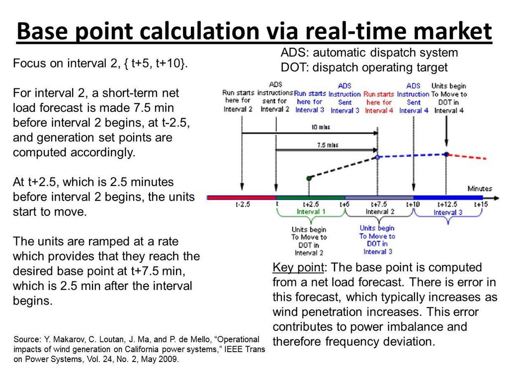
81 8 tie ref L tie m m T V T m ref G G V G V P K t KB t P t P M t P M t M D t P M t t P T t P T t P t P T t R T t P T t P t T t T t P tie 3.0 Bae point calculation A lat comment i that the ACE, being a meaure of how much the total ytem generation need to change, i allocated to the variou unit that comprie the balancing area via participation factor. Thi i illutrated in Fig. 9.5 of W&W. The participation factor are obtained by linearizing the economic maret dipatch about the lat bae point olution ee Wood & Wollenberg, ection 3.8. Bae point calculation i performed by the realtime maret every 5 min, a indicated in the lide at the top of the next page.

82 8

83 4.0 Control performance tandard Control Performance Standard CPS and CPS are two performance metric aociated with load frequency control. Thee meaure depend on area control error ACE, given for control area i a ACE i Pi Bf Pi APi SPi 3 where AP i and SP i are actual and cheduled export, repectively. ACE i i computed on a continuou bai. With thi definition, we can define CPS and CPS a CPS: It meaure ACE variability, a meaure of hortterm error between load and generation [ 6 ]. It i an average of a function combining ACE and interconnection frequency error from chedule [ 7 ]. It meaure control performance by comparing how well a control area ACE perform in conjunction with the frequency error of the interconnection. It i given by CF where CPS CF 00% 4a ControlParameter Month 4b ControlPar ameter ACE 0B min ute F min ute 4c 83

84 CF i the compliance factor, the ratio of the month average control parameter divided by the quare of the frequency target ε. ε i the maximum acceptable teady-tate frequency deviation it i 0.08 Hz=8 mhz in the eatern interconnection. It i illutrated in Fig. 9 [ 8 ]. ε -ε 60-ε 60+ε Fig. 9 [8] The control parameter, a MW-Hz, indicate the extent to which the control area i contributing to or hindering correction of the interconnection frequency error, a illutrated in Fig. 0 [8]. Fig. 0 [8] 84

85 If ACE i poitive, the control area will be increaing it generation, and if ACE i negative, the control area will be decreaing it generation. If F i poitive, then the overall interconnection need to decreae it generation, and if F i negative, then the overall interconnection need to increae it generation. Therefore if the ign of the product ACE F i poitive, then the control area i hindering the needed frequency correction, and if the ign of the product ACE F i negative, then the control area i contributing to the needed frequency correction. o A CPS core of 00% i perfect actual meaured frequency equal cheduled frequency over any - minute period o The minimum paing long-term -month rolling average core for CPS i 00% CPS: The ten-minute average ACE. In ummary, from [ 9 ], CPS meaure the relationhip between the control area ACE and it interconnection frequency on a one-minute average bai. CPS value are recorded every minute, but the metric i evaluated and reported annually. NERC et minimum CPS requirement that each control area mut exceed each year. CPS i a monthly performance tandard that et control-area-pecific limit on the maximum average ACE for every 0-minute period. The underlying iue here i that control area operator are penalized if they do 85

86 not maintain CPS. The ability to maintain thee tandard i decreaed a inertia decreae. 86

87 Appendix A Thee note are adapted from treatment in [0]. Speed governing equipment for team and hydro turbine are conceptually imilar. Mot peed governing ytem are one of two type; mechanical-hydraulic or Electro-hydraulic. Electro-hydraulic governing equipment ue electrical ening intead of mechanical, and variou other function are implemented uing electronic circuitry. Some Electro-hydraulic governing ytem alo incorporate digital computer oftware control to achieve neceary tranient and teady tate control requirement. The mechanical-hydraulic deign illutrated in Fig. A4 i ued with older generator. We review thi older deign here becaue it provide good intuitive undertanding of the primary peed loop operation. Baic operation of thi feedbac control for turbine operating under-peed correponding 87

88 to the cae of loing generation or adding load i indicated by movement of each component a hown by the vertical arrow. Fig. A4 A ω m decreae, the bevel gear decreae their rotational peed, and the rotating flyweight pull together due to decreaed centrifugal force. Thi caue point B and therefore point C to raie. Auming, initially, that point E i fixed, point D alo raie cauing high preure oil to flow into the cylinder through the upper port and releae of the oil through the lower port. The oil caue the main piton to lower, which open the team valve or water gate in the 88

89 cae of a hydro machine, increaing the energy upply to the machine in order to increae the peed. To avoid over-correction, Rod CDE i connected at point E o that when the main piton lower, and thu point E lower, Rod CDE alo lower. Thi caue a reveral of the original action of opening the team valve. The amount of correction obtained in thi action can be adjuted. Thi action provide for an intentional non-zero teady-tate frequency error. There i really only one input to the diagram of Fig. A4, and that i the peed of the governor, which determine how the point B move from it original poition and therefore alo determine the change in the team-valve opening. However, we alo need to be able to et the input of the team-valve opening directly, o that we can change the MW output of the 89

90 generator in order to achieve economic operation. Thi i achieved by enabling direct control of the poition of point C via a ervomotor, a illutrated in Fig. A5. For example, a point A move down, auming contant frequency, point B remain fixed and therefore point C move up. Thi caue point D to raie, opening the valve to increae the team flow. Fig. A5 A model for mall change We deire an analytic model that enable u to tudy the operation of the Fig. A5 controller 90

91 when it undergoe mall change away from a current tate. We utilize the variable hown in Fig. A5, which include ΔP C, Δx A, Δx B, Δx C, Δx D, Δx E. We provide tatement indicating the conceptual bai and then the analytical relation. In each cae, we expre an output or dependent variable a a function of input or independent variable of a certain portion of the controller..bai: Point A, B, C are on the ame rod. Point C i the output. When A i fixed, C move in ame direction a B. When B i fixed, C move in oppoite direction a A. Relation: xc Bx B Ax A A7.Bai: Change in point B depend on the change in frequency Δω. Relation: B xb A8 3.Bai: Change in point A depend on the change in et point ΔP C. Relation: AxA PC A9 Subtitution of A8 & A9 into A7 reult in xc P C A0a 9