THESIS SPATIAL VARIABILITY OF SNOW DEPTH MEASUREMENTS AT TWO MOUNTAIN PASS SNOW TELEMETRY STATIONS. Submitted by. Evan J. Blumberg

Transcription

1 THESIS SPATIAL VARIABILITY OF SNOW DEPTH MEASUREMENTS AT TWO MOUNTAIN PASS SNOW TELEMETRY STATIONS Submitted by Evan J. Blumberg Department of Geosciences In partial fulfillment of the requirements For the Degree of Master of Science Colorado State University Fort Collins, Colorado Fall 2012 Master s Committee: Advisor: Steven Fassnacht Melinda Laituri Greg Butters

2 Copyright by Evan J. Blumberg 2012 All Rights Reserved

3 ABSTRACT SPATIAL VARIABILITY OF SNOW DEPTH MEASUREMENTS AT TWO MOUNTAIN PASS SNOW TELEMETRY STATIONS Much of the Western United States relies heavily on spring snow melt runoff to meet its industrial, agricultural, and household water needs. Water professionals use the network of snowpack telemetry (SNOTEL) stations to help forecast spring melt water runoff. These stations only represent a small area and across a watershed, the variability in snowpack properties can be large. Properties such as snow depth can vary substantially even over distances as short as a meter. Previous studies have examined how snow depth is distributed across the landscape and how terrain and vegetation parameters can be used as surrogates for the meteorological variables that drive the distribution of snow. The parameters are derived from a digital elevation model (DEM) that is now at a 30 resolution, and they include elevation, aspect, slope angle, and canopy cover, as well as clear sky solar radiation and the maximum upwind slope. Typically three to five snow depth measurements are taken to represent each 30 m DEM pixel. This study examines the distribution of variability in snow depth within a pixel. Snow depth surveys were conducted around the Joe Wright SNOTEL station near Cameron Pass in northern Colorado on May 1 st, 2009 and May 1 2, 2010 and around the Togwotee Pass SNOTEL station in north central Wyoming on March 17 th Surveys were performed by taking snow depth measurements in a 1 x 1 kilometer block around each SNOTEL station. Due to the logistics of sampling these two locations that both have dense ii

4 forests and steep terrain, three different sampling methods were employed based on a standard of three points in a row spaced 5 meters apart. To examine the variability at a location (pixel), at least eight additional measurements were taken between the three points (11 points were taken on May 1 st, 2009 at Joe Wright). At Togwotee Pass, 10 additional depth measurements were taken about the mid point, perpendicular to the main transect, yielding 21 points. For the 2010 survey at Joe Wright, the 11 points in a row were supplemented by two points at the beginning, middle and end (three standard points) to yield 17 measurements at a location. From these data the parameters most strongly correlated with the average snow depth, the standard deviation of snow depth, and the coefficient of variation were computed. Binary regression trees were used to further explore the relation between the average and variability and the terrain and canopy parameters. The statistics (average and standard deviation) from the standard three points was compared to all the points (11, 17 or 21) measured at a location. Data were sub set from all the points to determine the average difference and subsequently an appropriate number of depth measurements that should be taken to represent a location. Key variables were not consistent for the 2009 and 2010 Joe Wright SNOTEL surveys, and also varied when looking at standard deviation or coefficient of variation. Among many surveys, canopy cover, elevation, and sin of slope were key variables, but to different degrees. Investigation into survey efficiency show that taking between 3 to 6 data points iii

5 per pre determined sample point is suitable to be within 5% of the overall average, whether it be the 11, 17, or 21 point survey scheme. Blumberg, E.J., Spatial Variability of Snow Depths Measurements at Two Mountain Pass Snow Telemetry Stations. Unpublished M.S. thesis, Department of Geosciences, Colorado State University, Fort Collins, Colorado, USA. iv

6 ACKNOWLEDGEMENTS Funding for the 2009 Joe Wright fieldwork was provided by a grant from the National Oceanic and Atmospheric Administration (NOAA Office of Hydrologic Development grant #NA07NWS ). The Togwotee Pass survey was undertaken by the Colorado State University (CSU) students enrolled in the WR575 (Snow Hydrology Field Methods) class over spring break Their work is acknowledged with thanks. The other surveys were undertaken by CSU student volunteers. Thanks are due to all those who helped in the field and those who digitized the data. v

7 TABLE OF CONTENTS 1.0 INTRODUCTION THE IMPORTANCE OF SNOW SNOWPACK PROPERTIES OPERATIONAL SNOW MEASUREMENTS PREVIOUS WORK PURPOSE OF THIS RESEARCH STUDY SITES SNOTEL STATION CHARACTERISTICS JOE WRIGHT SNOTEL STATION TOGWOTEE PASS SNOTEL STATION METHODS SAMPLING STRATEGIES INDEPENDENT VARIABLES Elevation Aspect a Eastness b Northness Slope Maximum Upwind Slope Clear Sky Solar Radiation Canopy Cover ANALYSIS AND STATISTICAL METHODS RESULTS POINTS COMPARISON INDEPENDENT VARIABLE CORRELATION BINARY REGRESSION TREES INTERANNUAL COMPARISON: JOE WRIGHT 2009 VERSUS SAMPLING METHODS DISCUSSION REGRESSION TREES JOE WRIGHT 2009 VERSUS HUMAN FACTORS SAMPLING STRATEGIES CONCLUSIONS AND RECOMMENDATIONS 50 REFERENCES 51 vi

8 Chapter 1 Introduction 1.1 THE IMPORTANCE OF SNOW In the Western United States, 50 to 80% of the water is derived from snowmelt (USDA NRCS, 2009). This snowmelt contributes to the water supply for drinking water, industry, and irrigation for more than 60 million people (Bales et al., 2006) with an estimated direct and in direct economic impact of 300 billion dollars annually (Cline pers. comm., 2000). In California, 75% of the state s water for agriculture was derived from snowmelt from the Sierra Nevada Mountains (Molotch et al., 2005), while in Colorado waters derived from snow melt along the Continental Divide are not only vital to that state but also to the midwest and far western United States (Campbell et al., 1995). With so much reliance on snowmelt water, it is crucial to have the accurate estimates of amount of snow in the mountains and the subsequently runoff each season for water supply as well as flood preparation and mitigation. 1.2 SNOWPACK PROPERTIES Snow water equivalent (SWE) is the total amount of water that is in the snowpack and is very important for estimating spring snowmelt amounts < However, snow depth (ds) is the easiest snowpack property to measure. SWE is the product of ds and the depth averaged snowpack density (ρs), and ρs has been seen to be less spatially variable than SWE or depth (Logan, 1973; Fassnacht et al., 2010). 1

9 1.3 OPERATIONAL SNOW MEASUREMENTS In the 1930s, the Natural Resource Conservation Service (NRCS) started the snowcourse network across the Western United States to measure snow depth and SWE on a monthly basis, usually from January through June. Typically 10 to 15 snow samples were taken manually by extracting a snow core over a 100 to 300 m transect (USDA NRCS, 2009). The SWE data have been used by the NRCS and the National Weather Service to forecast spring and summer runoff volumes. In the late 1970s, the snowpack telemetry (SNOTEL) network was established to automate the snowpack and related measurements in the often remote mountain watersheds. Numerous snowcourse sites have been replaced by collocated SNOTEL stations. The SNOTEL stations deliver data in real time using meteor burst technology. This involves sending and bouncing radio signals off an ionized meteor band 50 to 75 miles above the Earth, without the use of satellites (USDA NRCS 2009). SNOTEL stations record hourly snow depth, snow water equivalent (SWE), precipitation totals, air temperature, and other hydro climatic data at some stations in real time. SWE is collected by a pressuresensing snow pillow while snow depth is measured using an ultrasonic depth sensor. The snowcourse and SNOTEL network are useful to provide reference points to estimate runoff volumes, but the manual snowcourse measurements are only collected monthly and while the SNOTEL data have an adequate temporal resolution to represent the dynamic evolution of the snowpack, they only represent a small area (~10 m 2 ). To understand the distribution of snow, manual field surveys have been conducted across various small alpine watersheds (e.g., Elder et al., 1991; Balk and Elder, 2002; Erickson et al., 2

10 2005; Molotch and Bales, 2005; Hultstrand et al., 2006). However, almost all snowcourse and SNOTEL sites arelocated in forested areas, and the SNOTEL stations tend not to be representative of the area surrounding them (Molotch and Bales, 2005). Rice and Bales (2010) suggested that a network of sensor should be used to provide a better estimate of snow depth. 1.4 PREVIOUS WORK Numerous studies have estimates snow depth across an area based using different statistical techniques (e.g., Erxleben et al., 2002). Since the distribution of snow is difficult to measure at a fine scale, various spatial terrain and vegetation variables are often used as a surrogate for the meteorology that drives the variability in snowpack properties. Elevation, slope, aspect, net clear sky solar radiation, and vegetation was used to estimate the distribution of snow depth at several Rocky Mountain sites in Colorado for the NASA Cold Land Process Experiment using five statistical models, including inverse distance weighting, kriging, modified residual kriging, cokriging, and binary regression trees (Erxleben et al., 2002). Each models left some spatial variability unexplained, with the binary regression trees being the most successfulexplaining 18 30% of the variability in the snowpack at the studied sties. For alpine areas, wind related factors influence the distribution of snow depth so Winstral et al. (2002) created the maximum upwind slope and topographic break parameters from a digital elevation model (DEM) as surrogates for wind sheltering and drifting. For part of Niwot Ridge Colorado, these wind variables plus elevation, slope and 3

11 solar radiation were all found to be statistically significant in predicting snow depth, with the index of wind sheltering the most significant (Erickson et al., 2005). In an alpine basin of the Sierra Nevada Mountains of California, the spatial distribution of snow water equivalent (SWE) in an alpine basin was primarily controlled by elevation and maximum upwind slope (Molotch et al., 2005). 1.5 PURPOSE OF THIS RESEARCH In a study in Northern Saskatchewan Canada,Neumann et al. (2006) concluded that one single fixed point measurement (such as a SNOTEL station) is not a statistically useful tool to represent the average snow depth of an area, even with a relatively uniform snow pack. For areas of interest that cannot be surveyed manually, multiple automated sensors can be used to increase the accuracy of snow estimates for a particular basin mean within 25% using 1 to 44 sensors, with an average of 5, depending on the snow variability of the basin. More sensors are likely needed to achieve the same accuracy in a more topographically variable study area (Neumann et al., 2006). The goal of this research is to determine how many sampling points are needed to measure a representative snow depth. López Moreno et al. (2011) sampled 121 points at 15 relatively homogenous 100 m 2 plots in the Spanish Pyrenees Mountains. They found that five to seven points produced an average snow depth within 5% of the 121 points. The sampling conducted in this research collected fewer points at each plot (hereinafter called a sampling location) but increased the number sampling location (per day) to more than 130.Each survey used a different number of measurement points at each sampling location 4

12 to exploring the practicality and efficiency of sampling, yet the same question remained: is there specific a number of measurement pointsat a sampling location after which extra depth measurements are not needed to yield a representative average? This question will help inform sampling strategies and survey efficiency, and can lead to a better understanding of snowpack variability. The absolute difference between the average of a sub set of measurement points and all points at a sampling location was computed. Statistically analyses were performed to identify the key terrain and canopy variables that determine the distribution and variability of snow depth around the two SNOTEL stations. The distribution of the snow was computed from the average of the depths at each sampling location, while the variability was computed from the standard deviation of depths per sampling location. The coefficient of variation was used as an integrator of the average and standard deviations. The independent variables included elevation, slope (sine of slope), northness (product of sine of slope and cosine of aspect to represent an integration of wind and sun influences with a steep north facing slope approaching a value of 1 and a steep south facing slope approaching a value of 1), eastness (product of sine of slope and sine of aspect to represent wind processes), cumulative monthly clear sky solar radiation, maximum upwind slope, and canopy density. The strength of the correlation between the independent variables and the snow statistics (average, standard deviation, coefficient of variation) were computed. The relation between these statistics was determined. Binary regression trees were also used to identify the sequence of variables necessary to distribute the average, standard deviation, and coefficient of variation of snow depth. 5

13 Through this research, it is hoped that snow surveys can be more accurate and efficient. Using different statistical methods to identify important factors contributing to snow pack depth will eventually help to determine snow depths over an area more accurately than a localized SNOTEL station, with less energy and time than a full snow survey. In future, models could be developed using the most important variables for a given area to determine the distribution of snow depth without manual measurements. 6

14 Chapter 2 Study Sites 2.1 SNOTEL STATION CHARACTERISTICS For this study, snow depth was measured manually around the Joe Wright SNOTEL station near Cameron Pass in northern Colorado and the Togwotee Pass SNOTEL station (2944 m above sea level) in northwest Wyoming (Figure 2.1). Both areas had extensive Spruce Fir forests. The canopy was more dense at Joe Wright than Togwotee Pass (Figure 2.2). The Togwotee Pass area mostly faced from degrees (south east to south west), while the Joe Wright area faced either degrees (east to south east) or (west to north) (Figures 2.3a and 2.3b). Snow depth data from the SNOTEL sites were compared with manualsnow depth measurements around the each station to determine the spatial variability in snow depths. Each snow surveys attempted to cover a 1 x 1 kilometer areaaround the SNOTEL station with 10 transects each separated by 100 meters. Plots were taken at 50 m intervals along each transect. The basic design was to determine the representivity of the SNOTEL station and the distribution of snow using the average of 3 points taken 5 meters apart (Meromy et al., 2012). All samples were taken at a 1 m interval. The Togwotee Pass survey, conducted on March 17, 2009, used 21 measurement points in a plus configuration (Figure 2.4a), at 159 locations. The May 2, 2009 survey at Joe Wright used 11 measurement pointsin a row (Figure 2.4b), at 203 locations, while the May 1 2, 2010 Joe Wright used 17 measurement points (Figure 2.4c), at 184 locations. This last survey had 11 measurement points in a row with 2 extra points at the beginning, middle and end. 7

15 2.2 JOE WRIGHT SNOTEL STATION The snow season at Cameron Pass (Joe Wright SNOTEL) was slightly above average with a peak SWE of 701 mm, compared to the 30 year average from of 681 mm (Figure 2.5). Peak SWE occurred on May 6, 2009, with the first snowfall occurring on October 12, 2008, first accumulation on October 22, 2008, and last day with snow on the ground being June 18, Snow depth peaked at 218 cm on April 19, In total, there were 246 days with snow on the ground, which is only 2.1 days less than the 30 year average. The snow season of at Joe Wright SNOTEL was below the average peak SWE at 658 cm on May 16, The first snowfall occurred on September 22, 2009, with accumulation beginning on October 5, The last day with snow on the ground was June 17, In total, there were 261 days with snow on the ground. The May 2, 2009 survey at Joe Wright covered a 1x1km block around the SNOTEL station, consisting of 11 points at 203 locations. The 11 points were in a north south direction spaced 1 meter apart. The May 1 2, 2010 survey featured the same 1x1km block around the SNOTEL site, but consisted of 17 points at 184 locations. It was composed of the same north south line, but had one point to the east and west at the end and center locations of the line. 2.3 TOGWOTEE PASS SNOTEL STATION The peak SWE for at the Togwotee Pass was 841mm, occurring on May 8, This peak is above the average from of 700 mm (Figure 2.5). The March 17,

16 Togwotee pass survey of 21 measurement points taken at 159 locations covered an area of 700 m x1 km around the SNOTEL station. At each measurement location, there was a center point with 4 arms going north, south, east, and west for 5 points 1 meter apart. The Togwotee Pass transects ran from west to east while the Joe Wright transects ran from north to south due to the nature of the terrain. Figure 2.1: Regional map of Togwotee Pass, WY and Cameron Pass, CO for the Joe Wright SNOTEL (Image from Google Earth). 9

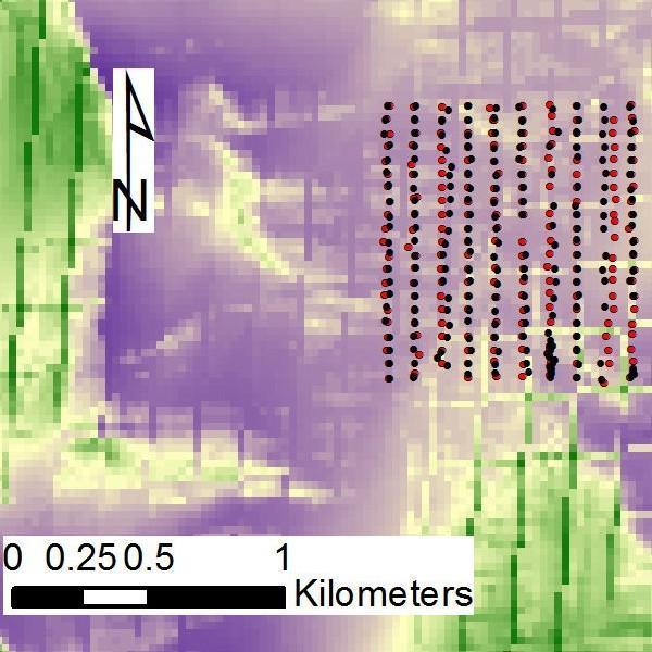
17 Frequency (Percent) Figure 2.2: Canopy density of Togwotee Pass (left) and Joe Wright (right) survey areas, with snow depth sampling locations shown (red=2009, black=2010 for Joe Wright) Joe Wright Togwotee Pass Aspect Figure 2.3a: The distribution of aspect around the Togwotee Pass and Joe Wright SNOTEL stations at the snow depth sampling locations. 10

18 Figure 2.3b: Aspect maps for Togwotee Pass (left) and Joe Wright (right) survey areas, with snow depth sampling locations shown (red=2009, black=2010 for Joe Wright). a) 21 point configuration b) 11 point configuration c) 17 point configuration X (0,+5) X X X X X (0,+5) X X X X X X X X (0,+5) X X X X X X X X X X X X X X X X X X ( 5,0) center center center X (0,0) (+5,0) X (0,0) X (0,0) X X X X X X X X X (0, 5) X (0, 5) X (0, 5) X X X Figure 2.4: Survey sampling scheme for a) Togwotee Pass (March 17, 2009) with 21 points and arms branching out in each direction; b) Joe Wright (May 1, 2009) with 11 points and arms in the north and south direction; and c) Joe Wright (May 1 2, 2010) with 17 points and arms in the north and south direction, plus one sample point to the east and west of the center point and each end point. 11

19 Peak SWE (mm) Joe Wright Togwotee Pass Figure 2.5: Peak SWE for water years at Togwotee Pass SNOTEL and at Joe Wright SNOTEL (data from < 12

20 Chapter 3 Methods 3.1 SAMPLING STRATEGIES During a snow sampling effort, eachsurveyor used a GPS unit to navigate to the start of a transect at a predetermined sample coordinate,and proceeded to follow their transect north south (Joe Wright survey) or east west (Togwotee Pass survey) at 50 m intervals. Each person was instructed to navigate to within 10 meters for any given coordinate, and record the GPS coordinates at the center point to the nearest one meter. A1 cm diameter aluminum probe(extendable in 1 meter lengths)was used to measure snow depth to the nearest one centimeter. All measurements that were anthropogenically influenced, such as a road or the snow bank beside a road was noted, and the data were not used in the analysis. A measure of the canopy cover (closed, partially closed, open, or no trees), and the GPS error were also recorded.the data were entered into an electronic spreadsheet shortly after each survey was performed. 3.2 INDEPENDENT VARIABLES Several variables were generated from the DEM using GIS software to examine their relationto average snow depth and variability. Canopy density was also used but this product was obtained directly. The following is a brief explanationof each variable used. 13

21 3.2.1 Elevation Elevation data (Figure 3.1) were obtained from the USGS 30 meter DEM< Data points were overlain onto the DEM in Arc Map GIS software, and elevation for each data point was then extracted and entered into a spreadsheet. Elevation is important in higher mountain such as Cameron Pass, since more precipitation (Dingman et al., 1988) and thus more snow (Fassnacht et al., 2003) is typically observed as elevation increases. Although this is the case, factors such as wind can scour high elevation areas, and deposit greater amounts of snow at lower elevations Aspect The aspect was determined for each point where snow depth was measured (Figures 2.2a and 2.2b). Aspect plays a very important role regarding snow depth, as it determines what areas get more or less sun throughout the winter and spring (Figure 3.2). At mid latitudes, such as Colorado and Wyoming, aspect is very important, as north facing areas will see little sun through the winter, while south facing snow can see a significant amount of sun. At high and low latitudes, aspect is not as important as the sun is either too weak to heavily affect the snow, or it is higher overhead, giving each aspect more consistent radiation a Eastness Since aspect is a merely bearing denoting the slope angle from 0 to 360 degrees, Eastnesswas computed as a measure of how east an area faces, and is defined as: Eastness = sine ( aspect n 180 ) x sine ( s1ope n ) (3.1),

22 as defined by Wallace and Gass (2008). Similar to aspect, eastness is important because of how much solar radiation a given area will receive. More easterly aspects will receive earlier sun, while the northerly aspects will receive less solar radiation overall b Northness Similar to eastness, northness is the measure of how north an area faces. It is defined as: Northness = cosine ( aspect n 180 ) x sine ( s1ope n ) (3.2), 180 as defined by Wallace and Gass (2008). It is important since it influences the amount of solar radiation that a given area will receive, i.e., the more an area faces north, the less sunlight it will see, keeping the snow colder, and thus taking more time to melt Slope Slope values were determined using GIS software for each snow depth data point (Figure 3.3). Slope can be important in steep areas, where snow can either sluff off or avalanche off down to lower slopes. This can have major impacts on snow depth and variability, as steep slopes may have lower snow depths, while shallow slopes in close proximity can be deeper due to the collection of the transported snow due to gravity. 15

23 3.2.4 Maximum Upwind Slope Maximum upwind slope is a parameter used to describe the topographic shelter or exposure relative to a specific wind direction (Winstral and Marks, 2002). This is particularly important as it describes the variability in snow deposition due to wind transport and redistribution (Molotchet al., 2005). It is defined as: SxA,dmax(xi,yi) = max (tan 1 { ELEV(sµ,µµ) ELEV (si,µi) [(sµ si)2+(µµ µi)2].j } ) (3.3), where A is the azimuth of the search direction, dmax controls the lateral extent of the search, (xi,yi) are the coordinates of the studied cell, (xy,yy) are the set of cell coordinates located along the line segment defined by A, dmax, and (xi,yi) (Winstral et al., 2002). In alpine areas such as Cameron Pass (Figure 3.4), and Colorado in general, wind can be responsible for stripping snow from westerly alpine areas and redistributing and loading it onto easterly aspects. This has a large impact on snow depth, as within a few meters, snow can be non existent to several meters in depth Clear Sky Solar Radiation Both snow survey locations of Cameron Pass and Togwotee Pass have unique solar radiation values for the month that the survey took place (Figure 3.5). This is a measure of the solar radiation impacting a specific area. Like aspect, this is important as it will impact the snow depth, as areas seeing more intense sun will melt (and consolidate) faster than areas that do not see as much sun. 16

24 3.2.6 Canopy Cover Canopy cover data were obtained from the USGS < and using GIS software the snow depth points were overlainon the canopy cover raster layer (Figure 2.1). Canopy cover is important, as it offers snow protection from the wind, and provides shade on sunny aspects. This can affect the snow depth, as a treed south facing slope may not be as melted out as an open south facing slope following a warm sunny spell. Protection from the wind can also keep the snow in place, keeping the snowpack deeper and preventing snow drifting and wind scouring. 3.3 ANALYSIS AND STATISTICAL METHODS From the snow depth data at each plot, average, standard deviation and coefficient of variation were calculated. Correlations between average snow depth, standard deviation, and coefficient of variation with each independent variable were calculated in the Microsoft Excel spreadsheet software. For each statistic and each study site/date, the independent variables were then ranked based on their correlation. Binary regression trees are an effective technique in identifying key variables affecting snow depth (Elder et al., 1991), and have been used to map the distribution of snow (Erxleben et al., 2002). Here regression trees were used to predict the key factors affecting average snow depth, standard deviation, and coefficient of variation. Regression trees were constructed in the statistical program R < project.org>. Reading through a binary regression tree starts with the root node at the top of the tree, which is also the most critical variable. The root node will consist of all data points 17

25 being regressed and an average overall value (snow depth average, standard deviation, or coefficient of variation for this study), as well as a value for the variable that is either less than, less than or equal, greater than, or greater than or equal. The tree then breaks down to less important variables in the same manner. When the variable is exhausted, there is a terminal node with the predicted value (snow depth average, standard deviation, or coefficient of variation) along with how many of the overall sample points are predicted to fall in that estimate. Comparisons of the 2009 and 2010 Joe Wright survey were conducted by overlapping both datasets to ensure that each corresponding data point from both years was actually at the same location, i.e., within the same pixel (pixels were approximately 30 m in size). A second comparison used points within one pixel to increase the number of comparable points between the 2009 and 2010 surveys. This enables highlighting similarities and differences between both years, including variability among the snowpack. To examine the impact of the number of sampling points per plot the average and standard deviation for the three (five for Togwotee Pass) points at the extremes of plot (+5, 5) were compared to the average and standard deviation of all points within a plot. Further, an average was computed starting with the one center point and adding points until all data points at a plot were used (moving outward from the center). These averages were compared to the overall average at each plot (11 measurement points for the 2009 Joe Wright survey, 17 measurement points for the 2010 Joe Wright survey, and 21 measurement points for the 2009 Togwotee Pass survey) to compute the absolute percent difference from the overall average. 18

26 Figure 3.1: GIS elevation data for the a) Togwotee Pass and b) Joe Wright survey areas, with snow depth sampling locations shown (red=2009, black=2010 for Joe Wright). Figure 3.2: The relation between aspect and latitude (from < 19

27 Figure 3.3: Slope data for the a) Togwotee Pass and b) Joe Wright survey areas, with snow depth sampling locations shown (red=2009, black=2010 for Joe Wright). Figure 3.4: Maximum upwind slope for the a) Togwotee Pass and b) Joe Wright survey areas, with snow depth sampling locations shown (red=2009, black=2010 for Joe Wright). 20

28 Figure 3.5: Solar radiation for the 2009 calendar snow year (October 15 April 15) for the a) Togwotee Pass and b) Joe Wright survey areas, with snow depth sampling locations shown (red=2009, black=2010 for Joe Wright). 21

29 Chapter 4 Results 4.1 POINTS COMPARISON For each survey, the average snow depth and standard deviation were compared for each sampling location (Figure 4.1a c and Table 4.1). For the Joe Wright 2009 survey, average snow depth fromthe three mainmeasurement points (center, northern most and southern most points in Figure 2.3) was almost the same as the average of all 11 measurement points with a Nash Sutcliffe efficiency coefficient (N S) of (Figure 4.1ai), while the three measurement point standard deviation was much less similar with an N S value of only (Figure 4aiii). There was no correlation between the average depth (from all 11 measurement points) and the standard deviation (Figure 4aii). Since 17 points were measured at Joe Wright in 2010 (Figure 2.3), the averages and standard deviations were compared from the three main points, as per Joe Wright 2009, the 11 points in a row, as per Joe Wright 2009, and all 17 points (Table 4.1). All the averages were similar (Figure 4.1bi) with all N S values being greater than 0.88, but the three versus 11 averages were less similar in 2010 than in 2009 with almost the same number of plots being collected each year (203 in 2009 and 206 in 2010). There was also less correlation with the standard deviations (negative N S value for 3 vs. 11 and 3 vs. 17) and again no correlation between average snow depth and the variation in snow depth presented as the standard deviation (Figure 4bii). A similar procedure was followed for the 2009 Togwotee Pass survey, with three, five (center, northern, southern, eastern, western most points), 11 and 21 points being considered (Figure 2.3). Three points produced similar averages as did 11 or 21 (N S of

30 and 0.831, respectively) and the five points also represented the 21 point average (N S of 0.904) (Figure 4.1ci). The standard deviation of the three points represented the 11 point standard deviation (N S of 0.222) better than the 21 point standard deviation (N S of 0.03) while the five points produced a better variability estimate compared to the 21 points (N S of 0.461). Again there was no correlation between the average and standard deviation of snow depth (Figure 4cii). 4.2 INDEPENDENT VARIABLE CORRELATION The correlations between the independent variables (Chapter 3.2) and average snow depth, standard deviation of the snow depth, and the coefficient of variation were computed and ranked (Tables 4.2a, 4.2b, 4,2c). Canopy density was negatively correlated to the average, the standard deviation and the coefficient of variation. Canopy density was more correlated to the average at Joe Wright than Togwotee Pass. Elevation was negatively correlated with the standard deviation and coefficient of variation for both sites. The sine of slope was negatively correlated to the coefficient of variation at both sites, and with the standard deviation at Joe Wright, but it is positive for Togwotee Pass. The more correlated independent variables were somewhat consistent having similar correlation strengths each year (at Joe Wright for 2009 and 2010), but there was less consistency for the correlations between the two sites.when 11 measurement points were used to compute the statistics for the same pixels sampled in 2009 and 2010, the independent variables correlated to average snow depth were almost identical (Table 4.3), with the relations being stronger in For the standard deviation the variables were less consistent with three of the top five being the same (solar radiation, sine of slope, and 23

31 maximum upwind slope), but in a different order. The order and strength of the relation for the coefficient of variation was more consistent as it followed the ranking for the average snow depth. For the 2010 sampling, all correlations were equal or stronger when only 11 measurement points were used compared to 17, with the ranking being in the same order as shown in Table 4.3 for the 11 points. Overall the independent variables were more correlated with the average and standard deviation at Joe Wright than at Togwotee Pass, although none of the individual correlations were strong; the largest correlation coefficient was (Table 4.2a). While it was not explored further, the location (UTM easting) was the most highly correlated variable at Togwotee Pass with the standard deviation ( 0.169) and coefficient of variation ( 0.142). 4.3 BINARY REGRESSION TREES Regression trees were constructed in the statistical program R for each snow survey to identify the most important variables affecting snow depth. Three binary regression trees were made for each survey: average snow depth, standard deviation of snow depth, and coefficient of variation. The following seven independent variables were used to generate: elevation, sine of slope, northness, eastness, canopy cover, solar radiation (May for Joe Wright surveys and March for Togwotee Pass survey), and maximum upwind slope. For each average snow depth regression tree, the independent variable and associated value are listed first, followed by the average snow depth (in centimeters), then by the number of data points being divided into each branch of the tree (Figures 4.2a c, 4.3a c, 4.4a c). At 24

32 each terminal nodes, the average snow depth and number of plots in the category are listed.the standard deviation and coefficient of variation regression trees are presented in the same manner, with the standard deviation or coefficient of variation listed in place of the average snow depth. The first and second nodes in each regression tree are summarized in Table 4.4. Variables used in the creation of the average snow depth regression tree for the Joe Wright 2009 survey were canopy cover (root node), elevation, northness, and sin of slope. When standard deviation of average snow depth is regressed, sin of slope (root node), canopy cover, eastness, May solar radiation, northness, and maximum upwind slope were used in the construction of the tree. When coefficient of variation is regressed, elevation (root node), canopy cover, eastness, maximum upwind slope, northness, and sin of slope were used in construction of the regression tree. The Joe Wright 2010 snow survey average snow depth regression tree was constructed using eastness (root node), canopy cover, elevation, northness, and sin of slope. The regression tree for standard deviation of average snow depth was constructed with sin of slope (root node), canopy cover, elevation, May solar radiation, northness, while the tree for coefficient of variation of average snow depth was constructed with elevation (root node), canopy cover, eastness, northness, and sin of slope. The Togwotee Pass snow survey average snow depth regression tree was constructed with the variables eastness (root node), canopy cover, maximum upwind slope, elevation, March solar radiation, and sin of slope. The regression tree for standard deviation of average snow depth was constructed with the variables elevation (root node), 25

33 sin of slope, maximum upwind slope, March solar radiation, and canopy cover. Key variables in the construction of the regression tree for coefficient of variation of average snow depth included elevation (root node), maximum upwind slope, sin of slope, canopy, and northness. 4.4 INTERANNUAL COMPARISON: JOE WRIGHT 2009 VERSUS 2010 To compare the May 2009 and May 2010 snow surveys at Joe Wright, measurement plots were identified that were centered on the same DEM pixel which has a resolution of 30 m, yielding 99 measurement plots (~50% of all plots) that were on pixels that same pixel between the two years. The correlation with independent variables is presented in Table 4.3 and was discussed above. Seventy additional measurement plots were identified that were within one pixel, with 13 more that were within 2 pixels from year to year. Only the same pixels and then within one pixel measurements were compared in terms of the average, standard deviation and coefficient of variation. Average snow depths were not well correlated (Figure 4.5a) between the two years for the same pixels (an R 2 value of 0.260) and even less correlated for all 176 plots at the same pixel or with one pixel (an R 2 value of 0.114). The slope of the line relating the two years was only 0.50 and 0.32 for the same and all pixels, respectively. The standard deviations were less correlated between the years (Figure 4.5b) than the average (an R 2 value of and for the same and all pixels) with shallow slopes (0.21 and 0.22). The coefficient of variation compared similarly (Figure 4.5c) with an R 2 value of and 0.110, and slopes of 0.32 and 0.37 for the same and all pixels. 26

34 4.5 SAMPLING METHODS Due to sampling logistics, the Togwotee Pass survey included 21 measurement points while the Joe Wright survey used only 11 points in 2009 and 17 in 2010, but will all points being 1 m apart. The average computed for all measurement points at each location was assumed to be the true snow depth for a particular pixel. To determine how many measurement points were needed to represent the true snow depth, the snow depth at the center point was compared to the average of all points. The mean absolute difference between the one point and all points was computed. The number of measurement points used to compute the average was increased by one and again compared to the all point average. This was repeated until all measurement points were used in the average. The absolute percent difference plotted versus the number of points illustrates that as more points are added, the deviation from the true snow depth decreases (Figure 4.6a). Since the total number of measurement points varied (11, 17, 21), the number of points to be within 5% of the true snow depth (as suggested by López Moreno et al., 2011) increased between the two Joe Wright surveys (Table 4.5). Examining these differences as a function of the percentage of total points (Figure 4.6b) shows that the deviation decreases most for the first few points then decreases at the same linear rate for both Joe Wright surveys. Togwotee Pass was less variable between 20 and 50% of the points included in the average. 27

35 Table 4.1: Nash Sutcliffe efficiency coefficient for the comparison between a different number of measurement points per plot for the average and standard deviation at Joe Wright (2009 and 2010) and Togwotee Pass. These values correspond to Figure 4.1a c i and iii. location and date points comparison average snow depth standard deviation Joe Wright vs Joe Wright vs Joe Wright vs Joe Wright vs Togwotee Pass vs Togwotee Pass vs Togwotee Pass vs Table 4.2a: Top five correlations (with correlation coefficient) for average snow depth, standard deviation, and coefficient of variation for Joe Wright in rank average snow depth standard deviation coefficient of variation 1 canopy density ( 0.171) sine of slope ( 0.265) sine of slope ( 0.274) 2 northness (0.152) elevation ( 0.190) elevation( 0.244) 3 eastness(0.131) canopy density ( 0.150) canopy density ( 0.134) 4 solar radiation( 0.131) max upwind slope(0.088) max upwind slope (0.123) 5 elevation (0.120) solar radiation (0.079) solar radiation (0.119) /eastness ( 0.190) Table 4.2b: Top five correlations (with correlation coefficient) for average snow depth, standard deviation, and coefficient of variation for Joe Wright in rank average snow depth standard deviation coefficient of variation 1 elevation (0.207) elevation ( 0.239) elevation( 0.273) 2 canopy density ( 0.161) sine of slope ( 0.208) sine of slope ( 0.209) 3 northness (0.101) maxupwind slope(0.149) max upwind slope (0.136) 4 sine of slope(0.093) canopy density ( 0.128) northness ( 0.113) 5 eastness ( 0.085) solar radiation (0.106) solar radiation (0.113) Table 4.2c: Top five correlations (with correlation coefficient) for average snow depth, standard deviation, and coefficient of variation for Togwotee Pass in rank average snow depth standard deviation coefficient of variation 1 eastness (0.236) canopy density ( 0.075) eastness ( 0.080) 2 max upwind slope(0.160) elevation ( 0.061) elevation( 0.043) 3 sine of slope (0.101) sine of slope (0.049 solar radiation ( 0.032) 4 canopy density ( 0.097) solar radiation ( 0.033) canopy density( 0.025) 5 solar radiation ( 0.034) northness (0.033) northness (0.024) 28

36 Table 4.3: Top five correlations (with correlation coefficient) for the measurements at the same pixel using 11 points between 2009 and 2010 (99 pixels) at Joe Wrightfor average snow depth, standard deviation, and coefficient of variation. rank average snow depth standard deviation coefficient of variation elevation (0.206) elevation (0.318) northness ( 0.139) elevation ( 0.242) northness ( 0.186) elevation ( 0.286) canopy density ( 0.169) canopy density ( 0.177) solar radiation (0.128) sine of slope ( 0.218) elevation( 0.182) sin of slope ( 0.208) northness (0.144) sine of slope (0.170) eastness ( 0.126) canopy density ( 0.208) sin of slope ( 0.179) max upwind slope (0.190) solar radiation( 0.126) northness (0.122) sine of slope ( 0.123) max upwind slope(0.200) eastness ( 0.178) northness ( 0.173) eastness (0.125) solar radiation ( 0.099) max upwind slope(0.102)solar radiation (0.175) solar radiation (0.177) solar radiation (0.162) Table 4.4: Binary regression tree summary table, with variable at first root node and second node split for each tree. location and variable first/root node split second node split date Joe Wright 2009 Average Snow Depth Canopy Elevation Joe Wright 2009 Standard Deviation Sin of Slope Canopy Joe Wright 2009 Coefficient of Variation Elevation Canopy, Maximum Upwind Slope Joe Wright 2010 Average Snow Depth Eastness Eastness, Northness Joe Wright 2010 Standard Deviation Sin of Slope Canopy Joe Wright 2010 Coefficient of Variation Elevation Sin of Slope, Canopy Togwotee Pass Average Snow Depth Eastness Canopy Togwotee Pass Standard Deviation Elevation Sin of Slope, Elevation Togwotee Pass Coefficient of Variation Elevation Maximum Upwind Slope, Elevation Table 4.5: Average number and percentage of points per plot to achieve less than a 5% absolute difference from the average computed using all points per plot. location and date # of Points to be Within 5% Threshold % of Points to be Within 5% Threshold % Difference from Total Points Joe Wright of % 4.4% Joe Wright of Togwotee Pass 4 of

37 Figure 4.1: Comparison of i) 3 point average versus all points, ii) standard deviation vs. average and iii) 3 point standard deviation versus all pointsfor a) Joe Wright in 2009, b) Joe Wright in 2010, and c) Togwotee Pass in

38 Canopy cm n = 203 Elevation < cm n = cm n = 15 Sin Slope cm n = 73 Elevation < cm n = 115 Northness < cm n = cm n = 17 Northness < cm n = cm n = 16 Canopy < cm n = cm n = cm n = 30 Canopy cm n = 69 Northness cm n =25 Canopy cm n = cm n = cm n = cm n = cm n = cm n = cm n = 8 Figure 4.2a: Joe Wright 2009 regression tree for average snow depth. Boxes without a variable represent a terminal node, with the average snow depth and how many points fit in that category. 31

39 Sin Slope n = 203 Canopy n = n = 7 Sin Slope n = 132 Eastness < n = 64 May Sol Rad < 6..57e n = n = 13 Eastness n = 35 Sin Slope n = 29 Sin Slope < n = 107 Northness < n = n = n = 8 Max Upwind Slope n = n = 10 Max Upwind Slope < n = n = n = n = n = 26 Northness n= n = n = n = n = 27 Figure 4.2b: Joe Wright 2009 regression tree for standard deviation of average snow depth. Boxes without a variable represent a terminal node, with the average snow depth and how many points fit in that category. 32

40 Elevation n = 203 Canopy n = 140 Maximum Upwind Slope < n = 63 Sin Slope n = 118 Sin Slope n = 7 n =118 Sin Slope < n = 7 n =111 Northness n = 7 n =104 Max Upwind Slope < n = n = 7 n = n = n = 18 Max Upwind Slope < n = 40 Eastness n = n = 8 Sin Slope n = n = n = n = n = 10 Figure 4.2c: Joe Wright 2009 regression tree for standard deviation of average snow depth. Boxes without a variable represent a terminal node, with the average snow depth and how many points fit in that category. 33

41 Elevation n = 203 Canopy n = 140 Maximum Upwind Slope < n = 63 Sin Slope n = 118 Sin Slope n = 7 n =118 Sin Slope < n = 7 n =111 Northness n = 7 n = n = 94 n = 10 Max Upwind Slope < n = Sin Slope n = 16 n = Max Upwind Slope < n = 15 n = n = 40 Eastness n = 14 n = n = 18 n = n = 7 Figure 4.3a: Joe Wright regression tree for average snow depth. Boxes without a variable represent a terminal node, with the averagee snow depth and how many points fit in that category. 34

42 Sin Slope n = 184 Canopy n = 133 Sin Slope n = 91 Eastness n = 111 n = 80 Sin Slope < n = 10 n =70 Sin Slope n = 7 n =63 Sin Slope < n = n = 15 Canopy < n = 51 Elevation n = 27 Northness n = n = 11 May Solar Radiation 5.74e n = n = 28 n = n = 7 Sin Slope < n = n = n = n = n = n = 43 Figure 4.3b: Joe Wright regression tree for standard deviation of average snow depth. Boxes without a variable represent a terminal node, with the average snow depth and how many points fit in that category. 35

43 Elevation n = 184 Sin Slope n = 118 Canopy < n = 66 Canopy n = n = n = 13 Eastness n = n =11 Sin Slope n =80 Eastness n = 69 Northnesss n = n = n = n = 16 Canopy n = 46 Canopy < n = 30 Canopy n = n = n = n = n = n = n = 8 Figure 4.3c: Joe Wright regression tree for covariance of average snow depth. Boxes without a variable represent a terminal node, with the average snow depth and how many points fit in that category. 36

44 Eastness < cm n = cm n = 13 Canopy cm n = cm n = 18 Elevation < cm n = 74 Maximum Upwind Slope < cm n = 126 Eastness < cm n = 52 March Sol Rad < 2.278e cm n =21 March Sol Rad 2.34e cm n = 53 Elevation < cm n = cm n = cm n = cm n = cm n = 19 Sin Slope < cm n = cm n = 16 Eastness cm n = cm n = cm n = cm n = 16 March Solar Radiation < 2.4e cm n = cm n = cm n = 9 Figure 4.4a: Togwotee Pass 2009 regression tree for average snow depth. Boxes without a variable represent a terminal node, with the average snow depth and how many points fit in that category. 37

45 Elevation n = 156 Elevation < n = 75 Sin Slope n = 81 Sin Slope < n = n = 7 Maximum Upwind Slope n = n = 11 Maximum Upwind Slope n = Canopy 75 n = n = n = 16 n = n = n = 14 Elevation n = 41 Sin Slope < n = 27 March Solar Radiation < 2.4e n = n = n = n = n = 14 Figure 4.4b: Togwotee Pass 2009 regression tree for standard deviation of average snow depth. Boxes without a variable represent a terminal node, with the average snow depth and how many points fit in that category. 38

46 Eastness < cm n = cm n = 13 Canopy cm n = cm n = 18 Maximum Upwind Slope < cm n = 126 Elevation < cm n = 74 Eastness < cm n = cm n = 13 March Sol Rad 2.34e5 March Sol Rad < 2.278e cm n = cm n = 53 Elevation < cm n = cm n = cm n = cm n = 19 Sin Slope < cm cm n = 9 n = 44 Eastness cm n = cm n = cm n = 14 March Solar Radiation < 2.4e cm n = cm n = cm n = cm n = 9 Figure 4.4c: Togwotee Pass 2009 regression tree for covariance of average snow depth. Boxes without a variable represent a terminal node, with the average snow depth and how many points fit in that category. 39