BIAS-ADJUSTMENT TECHNIQUES FOR IMPROVING OZONE AIR QUALITY FORECASTS. US Environmental Protection Agency, RTP, NC 27711, USA

Transcription

1 BIAS-ADJUSTMENT TECHNIQUES FOR IMPROVING OZONE AIR QUALITY FORECASTS Daiwen Kang* $#, Rohit Mathur +, S. Trivikrama Rao +, and Shaocai Yu $ + Atmospheric Modeling Division, National Exposure Research Laboratory, US Environmental Protection Agency, RTP, NC 27711, USA $ Science and Technology Corporation, 10 Basil Sawyer Drive, Hampton, VA, USA *Corresponding author kang.daiwen@epa.gov Phone: (919) # Current address: Atmospheric Modeling Division, US EPA, Mail Drop E243-03, RTP, NC August 2007 Revised March 2008 Revised July 2008

2 ABSTRACT In this study, we apply two bias-adjustment techniques to help improve forecast accuracy by post-processing air quality forecast (AQF) model outputs. These techniques are applied to modeled ozone (O 3 ) forecasts over the continental United States during the summer of The first technique, referred to as the Hybrid Forecast (HF), combines the most recent observed ozone with model-predicted ozone tendency for the subsequent forecast time period. The second technique applied here is the Kalman Filter (KF), which is a recursive, linear, and adaptive method that takes into account the temporal variation of forecast errors at a specific location. Two modifications to the Kalman Filter are investigated. A key parameter in the KF approach is the error ratio, which determines the relative weighting of observed and forecast ozone values. This parameter is optimized to improve the prediction of ozone based on time series data at individual monitoring sites in the Aerometric Information Retrieval Now (AIRNow) network. The optimal error ratios inherent in the KF algorithm implementation are found to vary across space; however, comparisons of the resultant KF-adjusted forecasts using a single fixed value of this parameter with those using the optimal values determined for each individual site reveal similar results, suggesting that the uncertainty in the estimation of this parameter does not have a significant impact on the final bias-adjusted predictions. The KF post-processing is also combined with the Kolmogorov-Zurbenko (KZ) filter, which extracts the intra-day variability in the observed ozone time series; the results indicate a significant improvement in the ozone forecasts at locations in the Pacific Coast region, but not as much at locations across the rest of the continental U.S. domain. Both HF and KF bias-adjustment techniques help significantly reduce the systematic errors in ozone forecasts. For most of the global performance metrics examined, the KF 1

3 approach performed better than the HF method. For the given model applications, both methods are effective in reducing biases at low ozone mixing ratio levels, but not as well at the high mixing ratio levels. This is due in part to the fact that high ambient ozone levels occur much less frequently than low to moderate levels for which the current model exhibits a systematic high bias. Additionally, the 12 km model grid structure is often unable to adequately capture the magnitude of peak O 3 levels. Thus, these extreme events at discrete monitor locations are more difficult to predict. Keywords: Air Quality Forecast; Kalman Filter; KZ filtering, Bias-correction; Ozone; Air Quality Modeling 2

4 1. INTRODUCTION There is a growing need to accurately forecast air quality to alert sensitive populations of unhealthful levels of air pollution. Recent advances in computing technology have now made it possible to apply comprehensive numerical photochemical models to forecast air quality on regional to continental scales. The simulation of atmospheric processes will always be imperfect since model assumptions, data limitations, and an incomplete understanding of physical/chemical processes introduce errors into the simulation results. Since air quality observations are the only means to quantify the actual conditions of the environment, simulation results should be evaluated against observations to judge model performance. Also, since numerical simulations are based on the solution of differential equations (i.e, changes of quantities over time and space), even a perfect numerical model cannot be expected to reproduce the observations because the initial state of the atmosphere is imperfectly known and the short-term temporal variability in the driving meteorology and emissions are not accurately quantified. Assuming that the model is capable of simulating the changes from a given initial state reasonably well, the forecast accuracy may be improved by post-processing the model results using appropriate bias-adjustment techniques. The air quality forecast system (AQFS) (Otte et al., 2005), developed through the partnership between the National Oceanic and Atmospheric Administration (NOAA) and the U.S. Environmental Protection Agency (EPA), entails coupling the operational North American Mesoscale (NAM) weather prediction model (Black 1994; Rogers et al., 1996) with the Community Multiscale Air Quality (CMAQ) model (Byun and Schere, 2006). The NAM-CMAQ modeling system has been used to provide forecasts of surface-level ozone (O 3 ) mixing ratios since Comparisons of O 3 forecasts with observations reveal that even though the day-to-day variability in O 3 is simulated quite well, the model 3

5 has a tendency to consistently overestimates the O 3 mixing ratios at the lower end of the mixing ratio distribution. This suggests that the forecast results could be improved by combining observations with forecast biases to create a more accurate forecast. Utilization of a post-processing bias-adjustment method incorporates recent model forecasts with observations to adjust current model forecasts. Previous bias in the forecast values are used to estimate the systematic errors in the forecast. Conceptually, once the future bias has been estimated, it can be removed from the model forecast to produce an adjusted forecast. Such an adjusted forecast should be statistically more accurate than the forecast based on the raw model output. Model post-processing techniques were first used in weather forecasts, especially for precipitation forecasts (Glahn and Lowry 1972; One of the principal reasons for this is that despite decades of refinement and improvement, meteorological models still contain significant errors in model physics (Wilczak et al., 2006). Air quality models are likely to have even greater model errors since they utilize the meteorological model output and highly uncertain emission inventories as inputs to drive complex chemistry and transport calculations. Various bias-adjustment methods have been proposed to postprocess model outputs. Wilczak et al. (2006) and McKeen et al. (2005) used a so-called mean subtraction bias correction in which the mean bias estimated over the entire forecast period at each site was subtracted from O 3 forecast at each hour. Homleid (1995) applied the Kalman Filter (KF) to diurnal corrections of short-term surface temperature forecasts, and more recently Delle Monache et al. (2006) applied Kalman filter (KF) to O 3 forecasts at five monitoring stations in the Lower Fraser Valley, British Columbia, Canada, for a short forecast period. These studies showed that bias-adjustment techniques, especially KF, can improve forecast skills relative to the raw model forecasts and that the KF bias-adjustment technique can effectively reduce systematic errors in 4

6 model output. Besides its recent application in bias-adjustment for post-processing forecast atmospheric variables, KF technique has been extensively used in meteorology for data assimilation (Whitaker et al., 2004; Houtekamer et al., 2005; and Wang et al., 2007). In this study, we apply the KF bias-adjustment technique, along with another simple bias-adjustment technique (referred to as the Hybrid Forecast, HF) to examine their relative strengths and weaknesses. Time series of atmospheric O 3 mixing ratios are influenced by various physical forcings. These can be effectively decomposed into different spectral components representing the different scales of forcing using the Kolmogorov-Zurbenko (KZ) filter (Zurbenko, 1986; Rao and Zurbenko, 1994; Eskridge et al., 1997; Rao et al., 1997; Hogrefe et al., 2000, 2001 a and b; Biswas et al., 2001). Since models exhibit significantly varying skills in simulating these different forcings (Hogrefe et al., 2001b), we apply KF to the KZ-decomposed O 3 mixing ratio time series to generate a KF bias-adjustment variant. These techniques are applied to O 3 forecasts at over 1000 measurement locations over the continental U.S. for the forecast period 1 July to 30 September, The 3-month forecast period over the continental U.S. provides a unique data set to examine the performance of these methods since a wide range atmospheric conditions occurred during the summer of During this period, many O 3 episodes (daily maximum 8-hr O 3 mixing ratios greater or equal than 85 ppb were recorded 570 times at AIRNOW monitoring stations) were observed at different locations; consequently, this 3-month period provides a broad range of O 3 mixing ratios to test the performance of the bias-adjustment techniques. The objectives of this study are to: (1) evaluate the efficacy of the post-processing techniques to improve skill for real-time O 3 forecasts, (2) investigate the spatial and temporal characteristics of these techniques when applied to O 3 forecasts, (3) analyze the 5

7 impact of these techniques on the systematic and unsystematic errors in model forecasts, (4) examine the possible combination of KF with spectrally-decomposed intra-day forcing using the KZ filter and its impact on forecast errors, and (5) since the skill of the air quality model is inherently dependent on quality of the input data used, assess the skill of key meteorological variables to provide guidance on the performance criteria for air quality forecasts. 2. BIAS-ADJUSTMENT TECHNIQUES 2.1 Hybrid Forecast (HF) The Hybrid Forecast (HF) is based on the simple assumption that the model is capable of predicting the change in the pollutant mixing ratio from one day to the next due to changing in the synoptic or large-scale forcing. Thus, forecast accuracy at given monitoring locations can be improved by combining the observed value at the previous time (the most accurate representation of the previous state) with the forecasted change in the mixing ratio from the previous to current time. The current observation at a location serves as the true initial condition for the forecast, while the forecast change from the model at the same location reflects the change of state. Thus, the bias-adjusted hybrid forecast (HF t+ t ) for a future time (t+ t) can be represented as: HF t+ Δt = Ot + ( M t+ Δt M t ) (1) where O t are observations at time t, and M t+ t and M t are modeled ozone forecast values at time t+ t and t, respectively. Here t is 24 hours. 2.2 Kalman Filter Predictor Forecast (KF) 6

8 A detailed description of the KF algorithm can be found in Delle Monache et al. (2006). For the sake of completeness, we provide a brief description of the methodology in Appendix A1. As stated by Delle Monache (2006), the KF performance is sensitive to the error ratio σ / σ and there exists an optimal value of the ratio given the forecast model and the 2 η 2 ε observation at each specific location. Later in this paper, we discuss our methodology for estimating the optimal error ratios for all locations within the continental U.S. domain and their impacts on the bias-adjusted forecasts. 2.3 Kalman Filter along with Spectral Decomposition Since time series of atmospheric pollutant mixing ratios contain the influence of various physical/chemical forcings, it can be decomposed into different timescales using a variety of filtering techniques (Rao et al., 1997; Hogrefe et al., 2000; Hogrefe et al., 2003; Wise and Comrie, 2005). The Kolmogorov-Zurbenko (KZ) filter (Zurbenko, 1986; Eskridge et al.; 1997; Rao et al., 1997; and Hogrefe et al., 2000) is often applied to O 3 time series analysis (e.g. Rao and Zurbenko, 1994 and Hogrefe et al., 2000). A time series of hourly O 3 varies over a 3-month period can be spectrally decomposed into its intra-day (ID), diurnal (DU), synoptic (SY), and baseline (BL) components. The atmospheric processes that may contribute to O 3 intra-day variations include turbulent mixing, local NO titration from fresh emissions, fast-changing emission patterns during rush hours, rapid boundary-layer growth and decay, and change in wind speed and/or actinic flux on this time scale (timescale < 11 hrs). Hogrefe et al. (2000, 2001b) have shown that the intra-day forcing has little temporal structure. In addition, our analysis and that of Hogrefe et al. (2000) suggest that while the intra-day forcing is nearly time 7

9 invariant at a given location, it does exhibit significant spatial heterogeneity as further discussed in subsequent Section 5.2. For instance, we examined the standard deviation of the intra-day component at a few locations over the entire analysis period of our study, and found that over a diurnal cycle, it is generally only a few ppb for the hourly O 3 observations. In addition, time series of the O 3 intra-day component do not show any significant correlation with intra-day components of any meteorological variable (Chan et al., 1999). Comparisons of modeled and observed intra-day O 3 components by Hogrefe et al. (2000) further suggests that deterministic numerical models do not adequately simulate the intra-day variations embedded in the observations. To account for this inherent uncertainty in the deterministic models, we investigated a modified approach for the Kalman Filter application. In this extension of the KF technique, the intra-day variations embedded in both the hourly O 3 observations and forecasts are extracted using the KZ filter following the methodology outlined by Hogrefe et al. (2000). Since a detailed discussion of the KZ filter can be found in Eskridge et al. (1997) and Rao et al. (1997), only a brief description of the technique is outlined in Appendix A2. After the decomposition using the KZ filter with a window size of 3 hours and 3 iterations (KZ 3,3 ), there are 18 hours left per day for the intra-day components (the first and last 3 hours are left out due to the process of running average with KZ 3,3 ). Next, the respective intra-day component time series is subtracted from the original time series at the corresponding hour for both observations and model forecasts. This leaves the time series of those most influenced by diurnal, synoptic, and baseline forcings which numerical models try to capture. KF is then applied to the resultant observation and forecast time series devoid of intra-day forcing. Finally, the intra-day forcing of the corresponding hour extracted from prior day s observations is added to the KF-generated forecasts, and the daily maximum 8-hr O 3 mixing ratios for the adjusted forecasts are then estimated from the resultant 8

10 hourly time series. Conceptually, the methodology described above attempts to recognize the inherent difficulties in comparing and combining grid-average values with point measurements; the utilization of the KZ filter results in model and observation series of compatible modes, and thus facilitating the assessment of systematic model biases. 3. MODELING SYSTEM AND MEASUREMENT DATASETS 3.1 The ETA-CMAQ Air Quality Forecast System In 2006, the WRF-NMM replaced the Eta model as the National Weather Service s North American Mesoscale (NAM) weather prediction model. In the applications discussed here, the Eta model provided the meteorological fields for input to CMAQ (Otte et al., 2005). The processing of the emission data for various pollutant sources has been adapted from the Sparse Matrix Operator Kernel Emissions (SMOKE) modeling system (Houyoux et al., 2000) using input from the U.S. EPA national emission inventory. The Carbon Bond chemical mechanism (version 4.2) is used to represent the photochemical reactions. Detailed information on the transport and cloud processes used in the CMAQ is described in Byun and Schere (2006). For this application, surface-level O 3 mixing ratios are forecast over a domain covering the continental U.S. (Figure 1) using a 12-km horizontal grid set on a Lambert Conformal map projection. 22 vertical layers of varying thickness set on a sigma coordinate are used to discretize the vertical extent ranging from the surface to 100 hpa. The chemical fields for CMAQ are initialized using the previous forecast cycle. The primary Eta-CMAQ model forecast for next-day surface-layer O 3 is based on the current day s 12 UTC cycle. 9

11 3.2 Observations Hourly, near real-time O 3 observations (ppb) obtained from EPA s AIRNow measurement network are used in this study ( Over 1000 monitoring stations are available within the continental US domain (Figure 1) for O 3 for the three month period from July to September, Daily maximum 8-hr O 3 mixing ratios are often used for verification purposes and for other forecast products. Note that the 8-hr O 3 mixing ratios are calculated using a forward calculation method, i.e., the 8-hr O 3 mixing ratio at a current hour is the average of hourly O 3 mixing ratios of the current and the succeeding 7 hours and assigned as the value for the current hour. In calculating the 8-hr average values, if 4 hourly values within an 8-hr window are missing, then the corresponding 8-hr average value is treated as missing, and if half of the 8-hr average values are missing within a day, the daily maximum 8-hr mixing ratio for this day is treated as missing. The data set is screened for missing data before the bias-adjustment techniques are applied. If the hourly values or daily maximum 8-hr mixing ratios at a station are missing on three consecutive days, the station is dropped from the data set for bias-adjustment. In our applications of the bias-adjustment techniques, when observations are missing for a time step, the KF uses the last known bias for the same time step from an earlier day, while the HF uses the corresponding model forecast values at the same time step. 3.3 Verification Statistics The Root Mean Square Error (RMSE) is often used to evaluate model performance since it quantifies the magnitude of the error in the model (Fox, 1981). The RMSE can be estimated as: 10

12 RMSE = 1 N N i= 1 ( C m C (, i) ( o, i) ) 2 (2) where i is the ith paired (model-observation) data point, N is the total number of paired,data points, and C (m,i) and C (o,i) are the ith modeled and observed mixing ratios, respectively. Following Willmott (1981), the RMSE can be split into its systematic and unsystematic components by regressing linearly the modeled (C m ) and observed (C o ) mixing ratios to yield the best fit line: * = a bco C + (3) where a and b are the least-square regression coefficients of C m and C o. The systematic (RMSEs) and the unsystematic (RMSEu) components are estimated as: RMSEs = 1 N N i= 1 ( C * C( o, i) ) 2 (4) RMSEu = 1 N N i= 1 ( C * C( m, i ) ) 2 (5) Additional metrics such as the Mean Bias (MB) and Index of Agreement (IOA) (Willmott, 1981) are also used in model evaluation. MB is defined as: MB = 1 N N i= 1 ( C m C (, i) ( o, i) ) (6) The MB provides the information on overall overprediction/underprediction in the forecasts. IOA is defined as: IOA = 1 N i= 1 N i= 1 ( C ( Cˆ ( m, i) ( m, i) C + Cˆ ( o, i) ( o, i) ) 2 ) 2 (7) 11

13 where ˆ ( m, i) = C( m, i) C, o C( o, i) = C( o, i) C o C ˆ, and C is the mean observed mixing ratios. o IOA specifies the degree to which the observed deviations about Co correspond, both in magnitude and sign, to the predicted deviations aboutc. The value of IOA varies between 0.0 to 1.0, representing limits of complete disagreement to perfect agreement between the observations and predictions. o 4. IMPLEMENTATION OF THE KF AND ERROR-RATIO OPTIMIZATION 4.1 KF Implementation Even though both observations and model forecasts provide hourly O 3 mixing ratios, the daily maximum 8-hr O 3 mixing ratios are currently being used to characterize the severity of O 3 pollution. The KF bias-adjustment for the predicted daily maximum 8- hr O 3 can be applied in two ways. Method 1 involves calculating the daily maximum 8-hr O 3 mixing ratios using the original model forecast and observed time series and then applying the KF to these data. In this case, there is only one value per day at each site. Method 2 entails the application of the KF to the original hourly O 3 time series to develop a KF-adjusted hourly O 3 time series, which is then used to compute the daily maximum 8-hr O 3 from the adjusted hourly time series. Figure 2 displays the relationship between the daily maximum 8-hr O 3 mixing ratios from the two methods at a monitoring station in North Carolina; similar level of agreement between the two methods was also found at several other locations. Figure 2 illustrates that there is little difference between these two methods. Although either method can be used, Method 1 involves significantly fewer computations than Method Optimization of the Error-Ratio 12

14 As discussed in Section 2.2, previous studies suggest that the KF performance can be sensitive to the error ratio σ / σ, which dictates the manner in which the KF responds 2 η 2 ε to the variations in biases at prior steps. At each location, given the climatology (related to observations) and the modeling system, there exists an optimal error-ratio value to generate the best KF forecasts. Homleid (1995) tested three different values of the ratio (0.01, 0.06, and 0.16) for temperature forecast adjustment in Norway and found that the sensitivity to the specification of the error ratio value is low with respect to bias reduction; he ended up choosing a happy medium value of Delle Monache et al. (2006) used a ratio value of 0.01, which was also used in previous KF bias-adjustment for weather forecasts in that area, to conduct KF bias-adjustment for O 3 forecasts. Delle Monache et al. (2007) investigated the optimization of the ratio values for ensemble O 3 forecasts over eastern North America during the summer of Relatively few systematic studies have been conducted with regard to how this important parameter in KF application should be optimized and to quantify its impact on the performance of KF bias-adjustment over a wide range of atmospheric conditions and geographical regions. In this study, optimal values of the error ratio at each location were determined by applying the KF correction to forecast time series over the three month period with a range of error ratio values (from to 10 with increments of ). The location specific optimal error ratio was then determined as the value which yielded the minimum RMSE in the adjusted forecasts. Figure 3 displays the optimal values of the error-ratio at each location. As shown in Figure 3, the optimal error-ratio values vary spatially by four orders of magnitude from In the eastern part of the domain, especially in the Northeast, the values tend to be small and in the range of to 0.1 at majority of the locations. Larger error-ratio 13

15 values in the 1-10 range are noted in the Midwest and Pacific coast region. Higher optimal error ratio values generally occurred in the areas where the model didn t perform well. This indicates that the bias-adjustment forecasts are more sensitive to the latest observations (i.e. persistence dominates the adjusted forecasts), while lower optimal error ratio values occurred in areas where the model performed well during this period; this signifies that the model forecasts play a greater role in the adjusted forecasts (i.e. the model forecasts dominate the adjusted forecasts, or in other words, the model performs well in reproducing the observations). The model performed quite well in the eastern part of the domain, especially in the Northeast. For the western portion of the domain, especially in Pacific Coast, the model didn t perform as well as it did in the east, which may in part be attributed to a combination of effects associated with the current model grid resolution, which is not sufficient to resolve the complex mountainous terrain, highly-variable meteorological conditions, spatial and temporal variability in emissions, and consequently the evolution of sub-grid chemistry leading to O 3 formation. Although the estimated optimal error-ratio values exhibit large spatial variability, their impact on the performance of the KF-adjustment was found to be insignificant compared to using a fixed value of 0.06 (based on Homleid, 1995, which is close to the median value, 0.05, of the estimated optimum error ratios across all sites). This is illustrated in Figure 4 which compares the RMSE for the adjusted forecasts using a fixed versus variable optimal error ratio values. Figure 4a presents the RMSE values from the raw model forecasts, Figure 4b displays the RMSE values from KF forecasts with a uniform error-ratio value of 0.06 for all locations in the domain, while Figure 4c provides the RMSE values from KF forecasts using the optimal error-ratio value shown in Figure 3 for each location. The KF forecasts greatly reduce RMSE values at almost all locations within the domain (compare Figure 4a and 4b). However, little improvement is evident in 14

16 using the optimal error-ratio values compared to the case with a uniform value of 0.06 for all locations (compare Figures 4b and 4c). The reduction in RMSE values is less than 1% in going from a KF using a moderate error-ratio value to the optimal one. This suggests that an error-ratio value in the range of 0.01 to 0.1 can be uniformly applied to all locations in KF forecasts to achieve good performance; this, in turn, helps simplify the use of KF in practical applications. In the subsequent analysis, the error-ratio value of 0.06 is used for all the monitoring stations. 5. RESULTS 5.1 Bias-Adjustment for O 3 Forecasts Figure 5 presents an illustration of the impact of the application of the HF and KF bias adjusted O 3 forecasts relative to both the observations and the raw model at a representative monitoring station located in Fuquay-Varina, North Carolina (Site ID: ). In Figure 5a, the histograms of model forecasts and observations along with the probability density functions (PDFs) are displayed. Application of the KF and HF adjustment techniques bring the PDFs of forecast values much closer to the observations, with KF providing better match with the observed distribution than HF. The improvement of the bias-adjusted forecasts over the original forecasts is further illustrated in the time series comparisons shown in Figure 5b. Compared to the observations, the raw model tends to overestimates O 3 on almost all days at this station. Though, HF-adjustment technique tends to bring the forecast closer to the observation as compared to the raw model forecasts, spikes or overshoots relative to the observations are also apparent (e.g. times when the green dashed lines appear to overshoot the peaks and troughs in the observed time series). The KF-adjusted forecasts track the observations more closely than the other two despite some spikes when the model forecasts and/or the 15

17 observations exhibit dramatic changes from the prior days. The KF forecasts are closer to the raw model forecasts at the beginning and get trained to gradually converge towards to the observations within a few days (3 to 5 days in the case shown in Figure 5b). Similar trends are found at other monitoring sites. Figure 6 presents scatter plots of forecast and observed percentiles for the daily maximum 8-hr O 3 mixing ratios for all the stations within the continental US domain. In constructing this figure following Mathur et al. [2008], at each site the time-series of both measured and model (or bias-adjusted model) daily-maximum 8-hr average O 3 over a season was examined and percentiles of the distribution over the season were computed for both the model and the measurements. Scatter plots of specific percentiles of the mixing ratio distributions (median) of the model and observed time-series are then examined to assess the ability of the model to capture the spatial variability in frequency distributions of O 3 mixing ratios across the sites (cf. Mathur et al, 2008). At each monitoring site, we examined the various percentiles of raw model (or bias-adjusted model) O 3 mixing ratio predictions over a season and compared them with the corresponding percentiles from the measured time-series as illustrated in Figure 6. As illustrated in this figure, the raw model forecast tends to overestimate across all O 3 mixing ratio ranges. The application of the bias-adjustment techniques reduce the systematic overestimation, thereby providing a better match with the observed distributions as reflected by the reduced scatter about the 1:1 line (i.e., perfect prediction). The HF forecasts underpredict at the lower percentiles (especially 5 th percentile) but overpredict at the higher percentiles (95 th ). The KF forecasts are the best with the data points almost evenly distributed around the 1:1 line. However, there is more scatter at lower and upper percentiles than in the middle mixing ratio range; illustrating model s difficulty in simulating the outliers. 16

18 Comparisons of the distribution of monthly RMSE values of maximum 8-hr O 3 mixing ratios of the raw model, KF, HF, and persistence forecasts over all the monitoring stations within the continental US domain are presented in Figure 7. In the persistence forecast, today s observed O 3 mixing ratio at any monitoring location is used as tomorrow s forecast. As seen in the figure, RMSE values are largest for the raw model forecasts, lowest for the KF forecasts, and in between for the HF forecasts and persistence forecasts for the given period. When the forecasts are evaluated using global statistical measures like RMSE, the persistence forecasts performed as well as the raw model forecasts; however, when evaluated using non-global measures such as time series, model forecasts have better performance especially during conditions representing the onset and dissipation of O 3 episodes as well as changing meteorological conditions. The boxplots in Figure 8 show the distribution of the RMSE, and its systematic and unsystematic components in the predicted daily maximum 8-hr O 3 mixing ratios for the raw model, KF, and HF forecasts for all the stations within the continental US domain. The RMSE values are largest in the raw model forecasts and smallest in the KF forecasts. As expected, both KF and HF forecasts greatly reduce the systematic part of RMSE, but not the unsystematic component of RMSE. Figure 8 shows that the unsystematic component of RMSE in the bias-adjusted forecasts increased when compared with the raw model forecasts; these trends are associated with the formulation of the bias-adjustment methods. Since the HF forecast represents the sum of the previous day observation and the simulated change between the previous and current day, unsystematic errors can be further magnified in the calculation of the change of the model forecasts between two consecutive bias-adjusting time steps. For instance, random errors can be additive during add or subtract operations. For instance, if the error associated with each term, M t and M t+ t, in Equation (1) is E, then the combined error during the 17

19 operation M t+ t - M t could be of the order 2E. In Figure 8, the mean RMSEu of the raw model forecasts is Theoretically, the RMSEu in HF forecasts (associated with M t+ t - M t ) can be as high as ( ), and this is very close to the real value of The KF adjustment is specifically formulated to reduce the systematic errors. However, small random errors could be introduced during the iteration calculations as shown in Figure 8, though the magnitude is quite small (the mean RMSEu of KF is 9.73 compared with 8.86 in the raw model forecasts, and in the HF forecasts). Figure 8 reveals that while bias-adjustment techniques help reduce the systematic errors in model forecasts, some residual error still exists in the adjusted forecasts which is primarily constituted by the unsystematic or random errors. This residual error represents the stochastic error associated with the inherent variability in the observations which cannot be adequately resolved by deterministic grid models. It should be noted that while model estimates represent volume-average concentrations, observations reflect point measurements. Furthermore, any observation at a given time reflects an event out of a population whereas model estimate represents the population average. Therefore, when paired in space and time model predictions will always differ from observations. The index of agreement (IOA) is another metric that can be used to assess improvements resulting from the application of bias-adjustment methods. As shown in Figure 9, the IOA increased on average by 14% and 13% for the KF and HF forecasts, respectively, demonstrating an improvement over the raw model forecasts. 5.2 KF with Treatment for the Intra-day Component for O 3 Forecasts As illustrated in the analysis above, while the HF and KF bias adjustment methods can significantly reduce the systematic errors in model O 3 forecast, they cannot 18

20 reduce the errors that are associated with the model s inability to adequately represent the high-frequency/high-wave number portion of the evolving spectrum of observations. The intra-day component of O 3 time series to a large extent represents this short-term variability in the observations. Additionally, since the driving meteorological models also under represent the intra-day components of key variables such as winds and temperature (Hogrefe et al., 2001a), accurate simulation of the ID forcing for pollutant species by air quality models should not be expected. Consequently, we investigated an extension to the KF technique in which it was combined with the KZ-decomposed intra-day component (KFid) as described earlier in Section 2.3. Figure 10 displays the spatial distributions of IOA values for all the stations within the continental U.S. domain for the raw model, the KF, and the KFid forecasts. Higher IOA values are noted almost everywhere with the KF forecasts (Figures 10a and 10b). However, even though the IOA values increase (from red to yellow or from yellow to green) in the Pacific Coast (PC) region, they are still noticeably lower than those for the rest of the domain. Although the IOA values of the KFid forecasts increase in the PC region, there is little change across the rest of the domain (Figure 10c). This suggests that the KF modification with the treatment for intra-day component (KFid) is more effective for the PC region. As the majority of the monitoring stations in the PC region are located in California, further investigation of the performance of the KFid forecasts in California was performed. Figure 11 displays the distributions of the RMSE and its systematic and unsystematic components for the raw model, the KF, and the KFid forecasts at monitoring stations only in California. Similar to the trends noted in Figure 8 for the entire continental US domain, RMSE values are much reduced by the KF and KFid forecasts when compared with the raw model forecasts. In California, the KFid forecasts reduced the RMSE values further than the KF forecasts. The KF and KFid forecasts have 19

21 much smaller RMSEs than the raw model forecasts, but exhibit slightly larger RMSEu values. The improvement in model with the KF and KFid methods over the raw model forecasts is also indicated by the IOA values across the monitoring stations in California shown in Figure 12. The boxplots of IOA values in KF and KFid forecasts are similar with a slightly larger median IOA for KFid than that for KF. The impacts of the bias-adjustment techniques on categorical forecast performance (see Kang et al., 2005) is examined in Figure 13 which presents the False Alarm Ratio (FAR) and Hit Rate (H) for the three forecast methods for stations in California (Figure 13a) and stations across the rest of the domain (i.e., excluding California) (Figure 13b), respectively. In California, the raw model and the KF forecasts have similar hit rate (H), while the H increases from 15% to 32% when the KFid method is applied in California. The false alarm ratio (FAR) values are lower in the KF and KFid forecasts than in the raw model forecasts. For the rest of the domain, H is highest in the raw model forecasts, while no significant difference is noted between the KF and KFid forecasts. FAR is the largest in the raw model forecasts, but again is similar between the two bias-adjusted forecasts. These analyses raise an interesting issue on differing performance of the KFid methodology for California relative to the rest of the domain. Recall that in the KFid formulation (Section 2.3), the intra-day forcing from the raw model forecasts and observations are removed from the original time series prior to the application of the KF; the intra-day component extracted from the `prior day s observations for the corresponding hour is then added back to the resultant KF adjusted time series. The performance discrepancy arises from the differences in the intra-day components embedded in the observations and model forecasts. The relatively larger variations in the intra-day component in the west coast than in the east could result from a combination of 20

22 effects arising from complex topography, land-sea breeze transitions, spatial heterogeneity in emissions, and their impact on chemistry leading to O 3 formation and distributions in the region. This is further confirmed by the histograms and the fitted Gaussian PDFs of the O 3 intra-day component (Figure 14). Figure 14a presents both the observed (black) and forecast (red) histograms of the O 3 intra-day components and the corresponding PDFs for all monitoring stations located in CA while Figure 14b presents similar plot for all monitoring stations located in the eastern US. The intra-day forcing in observations in CA is a bit stronger (standard deviation ~ 4 ppb) than those at the eastern US sites (standard deviation ~ 3 ppb). However, the modeled intra-day forcing across the entire domain is similar (standard deveiation ~ 3 ppb). Because the intra-day forcing in the observations in CA has larger variability than that in the model forecasts, the KFid approach resulted in the noted improved performance in CA. 5.3 Limitations of bias-adjustment The results discussed so far are based on average characteristics, i.e., the RMSE and AOI values are calculated across the entire range of mixing ratios. Figure 15 displays the forecast RMSE (a, b) and MB (c, d) values as a function of different subranges of the observed mixing ratios for stations located in California (a, c) and stations in the rest of the modeling domain (b, d). For the locations in California, at lower mixing ratios (<50 ppb), the KF and KFid bias-adjustment techniques exhibit smaller RMSE values compared to both the raw model forecasts and the HF bias-adjustment forecasts. Within the range of ppb, the KF, KFid, and the raw model forecasts have similar RMSE values. When the observed mixing ratios are larger than 70 ppb, the KF and KFid biasadjustment method exhibits lower RMSE values than the raw model forecasts. The HF forecasts have the largest RMSE values across most of the mixing ratio range. For the 21

23 rest of the modeling domain, the KF and KFid bias-adjustment techniques perform similar across the entire mixing ratio range; when compared to the raw model, both techniques reduce RMSE values at lower mixing ratios (<50 ppb), have similar values within the range of ppb, and produce larger values when the observed mixing ratios are larger than 70 ppb. The HF bias-adjustment technique has lower RMSE values than the raw model forecasts, but higher than the KF and KFid forecasts at lower mixing ratio range; it produces the largest RMSE values at higher O 3 mixing ratio range. This indicates that the KF is only effective at the lower end of the mixing ratio distribution, while the HF has little impact on reducing RMSE values at any mixing ratio levels. An examination of the distribution of the mean bias (MB) across the observed mixing ratio ranges is presented in Figures 15 c and 15d; in California, the KFid forecasts exhibit the smallest MB values (closest to 0) across all mixing ratio ranges though the values are close to those in the KF forecasts. The MB values for HF forecasts are similar to the KF and KFid approaches. For the rest of the domain, the MB values are always lower in the bias-adjusted forecasts compared to the raw model forecasts. At lower mixing ratios (< 70 ppb) the air quality model tends to overpredict, while at higher mixing ratios (> 70 ppb) it underpredicts, suggesting that the behavior of the model forecast bias is non-linear across different mixing ratio ranges (Yu, et al., 2007; Appel, et al., 2007). Since the KF bias-adjustment method is a linear algorithm and since the majority of the data points are typically lower than 70 ppb, when the method is applied to such a data set it gets trained as a corrector for overpredictions. This correction tends to extend to the higher O 3 mixing ratio range, further magnifying the model underestimations at the higher mixing ratios as indicated by the larger negative MB in Figure 15. Therefore, in the applications discussed here the effectiveness of KF bias-adjustment on model forecasts is limited to the lower O 3 mixing ratio range. When the behavior of the model forecasts 22

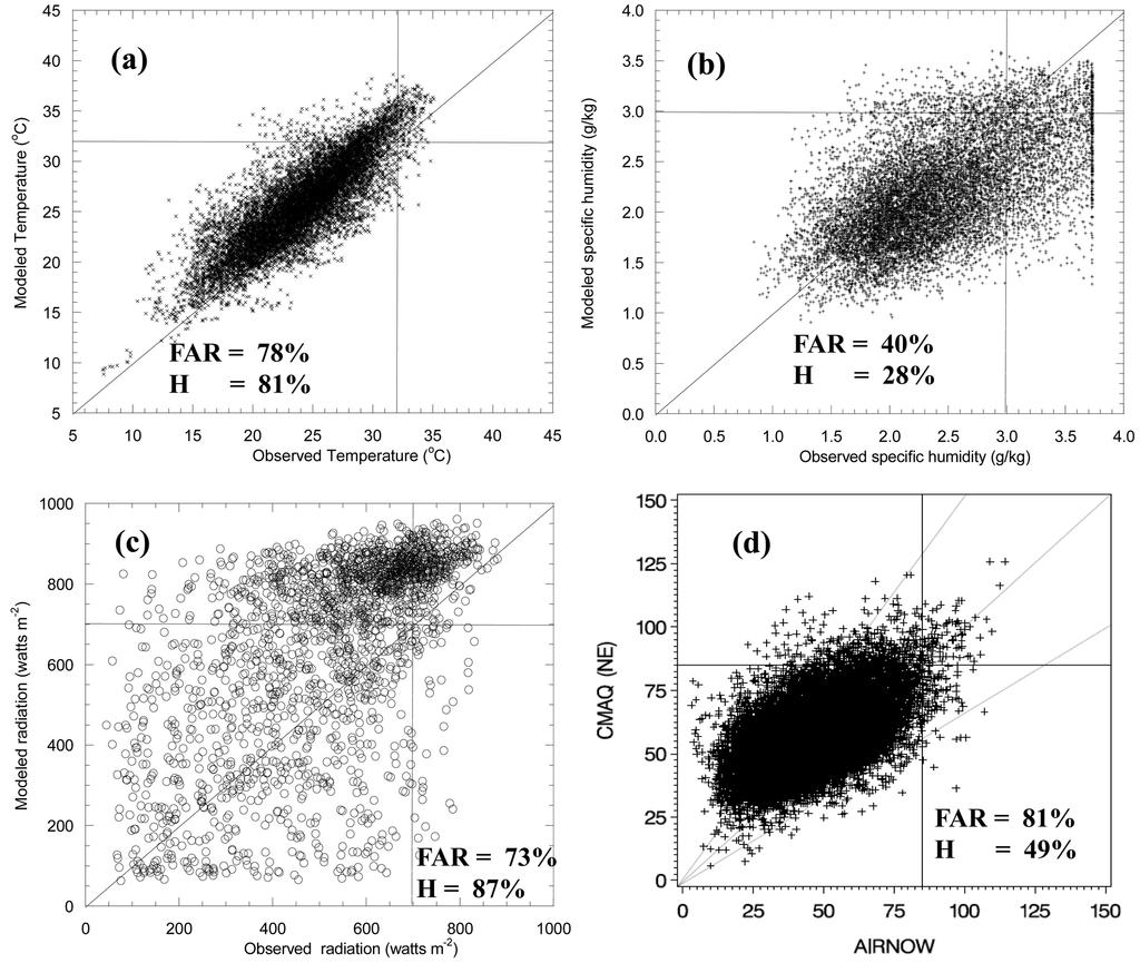
24 changes from one realm (overprediction) to another (underprediction), the KF approach is unable to respond to the change, resulting in the noted degradation of bias-adjusted forecast results. 5.4 Air Quality Forecast Accuracy: Practical Considerations Meteorological conditions and emissions information are the two primary inputs to air quality models; uncertainties associated with these inputs are propagated through air quality model calculations, affecting the O 3 mixing ratios output from the air quality model. From a practical standpoint, the prediction skill for these key input parameters must be considered in setting the performance criteria for the air quality prediction. Meteorological variables such as radiation, temperature, soil moisture, specific humidity, have a large impact on surface-level O 3 production. An illustration of the relative skills in predictions of meteorological and air quality variables is shown in Figure 16 which presents scatter plots of daytime (from 11:00 am to 4:00 pm Local Standard Time (LST)) hourly temperature, specific humidity, radiation, and daily maximum 8-hr O 3 mixing ratios for the period of July 2 to August 20, 2004 at locations across the northeastern U.S. To illustrate the performance of meteorological models in predicting extremes or episodic events, threshold values for temperature, specific humidity, and radiation are set at 32 ºC, 2.98g/kg, and 700 watts/m 2 (80% of the data range), respectively, while the threshold value for daily maximum 8-hr O 3 mixing ratio is set at the National Ambient Air Quality Standard (NAAQS) of 85 ppb for O 3. The categorical metrics, False Alarm Ratio (FAR) and Hit Rate (H), calculated based on these threshold values are shown in Figure 16. Note that if different threshold values are selected for the meteorological variables the corresponding categorical metrics may be slightly different 23

25 and also that the threshold values chosen for the meteorological variables do not directly correspond in any exact sense to the 85 ppb threshold value for O 3. Significant scatter between modeled and observed values is evident for all the variables in Figure 16, with a FAR of 78% and H of 81% for daytime temperatures, a FAR of 40% and H of 28% for daytime specific humidity, and a FAR of 73% and H of 87% for daytime mean radiation. The air quality predictions have a FAR of 81% and H of 49% for daily maximum 8-hr O 3 forecasts for the same time period. Since O 3 production is strongly dependent on these meteorological variables (i.e. temperature, moisture, cloud cover), the accuracy of model O 3 forecasts should be expected to be limited by the accuracy with which these key variables are simulated by the meteorology model. The results shown in Figure 16 illustrate that when the quality of air quality or meteorological predictions is assessed in this categorical sense of predicting an exceedance threshold, it is evident that the performance of meteorological and air quality models is comparable. 6. SUMMARY Air quality forecasts over a three-month period in 2005 are used to evaluate the merits of post-processing or bias-adjustment techniques. The results indicate that both Hybrid forecast (HF) correction and the Kalman filter (KF) predictor bias-adjustment methods can improve accuracy of model forecasts of O 3 by reducing forecast errors. For most of the global performance metrics examined, the KF approach performed better than the HF. Even though the estimated optimal error-ratios used in the KF approach vary from one location to another, the results presented here indicate that the impact of using spatially-varying optimal ratios (determined as those that resulted in least RMSE at the individual location) is marginal; a reasonable universal value within 0.01 to 0.1 would 24

26 present similar results for bias-adjustment of O 3 forecasts over the continental U.S. using the KF method. Although our analysis suggests that both the KF and HF methods can reduce the systematic errors significantly, the relative improvements from the application of these methods at peak O 3 mixing ratios were limited since the model exhibits differing bias characteristics at different mixing ratio ranges. For instance, for the model results examined here, a positive bias (overestimation) was noted at all mixing ratio ranges except when the maximum 8-hr O 3 > 70 ppb. Since the daily maximum 8-hr O 3 mixing ratios were predominantly in the < 70 ppb range, the adjustment methods tend to get trained for these conditions. Consequently, the application of the method to the higher O 3 mixing ratio range resulted in further magnifying the model s underpredictions at the high mixing ratio range. As a result, no appreciable improvement in the categorical forecast skills (the exceedance events for maximum 8-hr O 3 ) were noted with these biasadjustment techniques. However, modifications to the Kalman Filter technique with a time filtering technique accounting for the intra-day forcing at monitoring sites, result in improvements in categorical forecast skill metrics at locations in California. As indicated by our analysis, the reduction in RSME resulting from the application of the bias-adjustment techniques largely results from the reduction of the systematic component of the error. Much of the error (>70%) is associated with unsystematic errors, the magnitude of which cannot be reduced by these techniques. These unsystematic errors stem from the inability of the deterministic models to simulate the random component inherent in observations. The limitation of these bias-adjustment techniques is model-specific. It can be anticipated that if a model exhibits systematic biases (consistent overprediction or 25

27 underprediction across all O 3 mixing ratio ranges), these techniques should yield improvements greater than those noted here. In the applications presented in this study, the bias-adjustment techniques are only applied at discrete points, i.e., at location of the monitors. The extension of these methods for the development of bias-adjusted spatial maps (i.e., also at location where no monitor information is available) forecast surface-level O 3 distributions is an area for further research. Since surface-level O 3 distributions are influenced by local forcing associated with several meteorological drivers and spatially heterogeneous emissions, information on the spatial representativeness of the individual measurements and, consequently, the adjusted bias is critical to the extension of the methods presented here to develop biasadjusted spatial maps of O 3 forecast. The final performance of bias-adjusted forecasts depends on the performance of the model to which the bias-adjusted technique is applied. Since bias-adjusted techniques can only reduce systematic errors inherent in the model, additional improvements in model physics and chemistry are needed to reduce both systematic and unsystematic errors to further improve forecast performance. Additional research is also needed to develop methods to improve forecast accuracy for higher mixing ratios since they are most important from the human health and air quality regulations perspectives. 7. ACKNOWLEDGEMENTS The authors are grateful to Drs. Brian Eder and Kristen Foley for their constructive and insightful comments on initial drafts of this manuscript. We thank Drs. Luca Delle Monache and Roland B. Stull for providing their original Kalman Filter code. This manuscript has greatly benefited from extensive constructive suggestions of three anonymous reviewers. The research presented here was performed under the 26

28 Memorandum of Understanding between the U.S. Environmental Protection Agency (EPA) and the U.S. Department of Commerce's National Oceanic and Atmospheric Administration (NOAA) and under agreement number DW This work constitutes a contribution to the NOAA Air Quality Program. Although it has been reviewed by EPA and NOAA and approved for publication, it does not necessarily reflect their policies or views. 27

29 8. REFERENCE Appel, K.W., A.B. Gilliland, G. Sarwar, R.C. Gilliam, 2007: Evaluation of the Community Mulitiscale Air Quality (CMAQ) model version 4.5: Uncertainties and sensitivities impacting model performance; Part I ozone, Atmospheric Environment, in press. Black, T. 1994: The new NMC mesoscale Eta Model: Description and forecast examples. Wea. Forecasting, 9, Biswas, J. and Rao, S.T., 2001: Uncertainties in episodic ozone modeling stemming from uncertainties in meteorological fields. Journal of Applied Meteorology 40, pp Byun, D.W. and K.L. Schere, 2006: Review of the governing equations, computational algorithms, and other components of the Models-3 Community Multiscale Air Quality (CMAQ) modeling system. Appl. Mech. Rev., 59, Byun, D.W. and J.K.S. Ching, Eds., 1999: Science algorithms of the EPA Models-3 Community Multiscale Air Quality (CMAQ) modeling system, U.S. Environmental Protection Agency, EPA-600/R-99/030, 727 pp. Chan, D., S.T. Rao, I.G. Zurbenko, and P.S. Porter, 1999: Linking changes in ozone to changes in emissions and meteorology. Proc. Air Pollution 99 Conf., Palo Alto, CA, Wessex Institute of Technology, Delle Monache, L., T. Nipen, X. Deng, Y. Zhou, and R. Stull, 2006: Ozone ensemble forecasts: 2. A Kalman filter predictor bias correction, J. Geophys. Res., 111, D05308, doi: /2005jd Delle Monache, L., J. Wilczak, S. Mckeen, G. Grell, M. Pagowski, S. Peckham, R. Stull, J. Mchenry, and J. McQueen, 2007: A Kalman-filter bias correction method applied 28

30 to deterministic, ensemble averaged, and probabilistic forecasts of surface ozone, in press, Tellus B. Eder, B., D. Kang, R. Mathur, S. Yu, and K. Schere, 2006: An operational evaluation of the Eta-CMAQ air quality forecast model, Atmospheric Environment, 40, Eskridge, R. E., J.-Y. Ku, S. T. Rao, P. S. Porter, and I. G. Zurbenko, 1997: Separating different scales of motion in time series of meteorological variables, Bull. Amer. Meteor. Soc., 78, Fox, D. G., 1981: Judging air quality model performance: A summary of the AMS Workshop on Dispersion Model Performance, Bull. Amer. Meteor. Soc., 62, Glahn, H. R. and D. A. Lowry, 1972: The use of model output statistics (MOS) in objective weather forecasting, J. Appl. Meteor., 11, Hogrefe, C., S. T. Rao, I. G. Zurbenko, and P. S. Porter, 2000: Interpreting the information in ozone observations and model predictions relevant to regulatory policies in the eastern United States, Bull. Amer. Meteor. Soc., 81, Hogrefe, C., S. T. Rao, P. Kasibhatla, G. Kallos, C.J. Tremback, W. Hao, D. Olerud, A. Xiu, J. McHenry, and K. Alapaty, 2001a: Evaluating the performance of regionalscale photochemical modeling systems: Part I meteorological predictions, Atmospheric Environment, 35, Hogrefe, C., S.T. Rao, P. Kasibhatla, W. Hao, G. Sistla, R. Mathur, and J. Mchenry, 2001b: Evaluating the performance of regional-scale photochemical modeling systems: Part II ozone predictions, Atmospheric Environment, 35, Hogrefe, C., S. Vempaty, S. T. Rao, P. S. Porter, 2003: A comparison of four techniques for separating different time scales in atmospheric variables, Atmospheric Environment, 37,

31 Homleid, M., 1995: Diurnal corrections of short-term surface temperature forecasts using Kalman filter, Weather Forecasting, 10, Houtekamer, P.L., H.L. Mitchell, G. Pellerin, M. Buehner, M. Charron, L. Spacek, and B. Hansen, 2005: Atmospheric data assimilation with an Ensemble Kalman Filter: Results with real observations, Mon. Weather Rev., 133, Houyoux, M.R., J.M. Vukovich, C.J. Coats Jr., N.M. Wheeler, and P.S. Kasibhatla, 2000: Emission inventory development and processing for the Seasonal Model for Regional Air Quality (SMRAQ) project. J. Geophys. Res., 105, Kalman, R. E., 1960: A new approach to linear filtering and prediction problems, J. Basic Eng., 82, Kang, D., B.K. Eder, A.F. Stein, G.A. Grell, S.E. Peckham, and J. McHenry, 2005: The New England air quality forecasting pilot program: Development of an evaluation protocol and performance benchmark. J. Air Waste Manage. Assoc., 55, Mathur, R. S. Yu, D. Kang, and K. Schere, 2008: Assessment of the Winter-time Performance of Developmental Particulate Matter Forecasts with the Eta-CMAQ Modeling System, J. Geophys. Res., doi: /2007jd008580, 113, D McKeen, S., et al., 2005: Assessment of an ensemble of seven real-time ozone forecasts over eastern North America during the summer of 2004, J. Geophys. Res., 110, doi: /2005jd Otte, T.L., and Coauthors, 2005: Linking the Eta Model with the Community Multiscale Air Quality (CMAQ) modeling system to build a national air quality forecasting system. Wea. Forecasting, 20, Rao, S.T., I.G. Zurbenko, R. Neagu, P.S. Porter, J.Y. Ku, and R.F. Henry, 1997: Space and time scales in ambient ozone data. Bull. Amer. Met. Soc., 78,

32 Rao, S.T. and I.G. Zurbenko, 1994: Detecting and tracking changes in ozone air quality, J. Air Waste Manage. Assoc., 44, Roeger, C., R. B. Stull, D. McClung, J. Hacker, X. Deng, and H. Modzelewski, 2003: Verification of mesoscale numerical weather forecast in mountainous terrain for application to avalanche prediction, Weather Forecasting, 18, Rogers, E., T. L. Black, D. G. Deaven, G. J. DiMego, O. Zhao, M. Baldwin, N. W. Junker, and Y. Lin, 1996: Changes to the operational early Eta Analysis/Forecast System at the National Centers for Environmental Prediction. Wea. Forecasting, 11, Segers, A.J., H.J. Eskes, R.J. van der A, R.F. van Oss, and P.F.J. van Velthoven, 2005: Assimilation of GONE ozone profiles and a global chemistry-transport model using a Kalman filter with anisotropic covariance, Q. J. R. Meteorol. Soc., 131, Wang, X., T.M. Hamill, J.S. Whitaker, and C.H. Bishop, 2007: A comparison of hybrid ensemble transform Kalman filter-optimum interpolation and the ensemble square root filter analysis schemes. Mon. Wea. Rev., 135, Whitaker, J.S., G.P. Compo, X. Wei, and T.M. Hamill, 2004: Reanalysis without radiosondes with real observations. Mon. Wea. Rev., 132, Wilczak, J., S. McKeen, I. Djalalova, G. Grell, S. Peckham, W. Gong, V. Bouchet, R. Moffet, J. McHenry, P. Lee, Y. Tang, and G. R. Carmichael, 2006: Bias-corrected ensemble and probabilistic forecasts of surface ozone over eastern North America during the summer of 2004, J. Geophys. Res., 111, D23S28, doi: /2006jd Willmott, C. J., 1981: On the validation of models, Phys. Geogr., 2, Wise, E.K. and A.C. Comrie, 2005: Meteorologically adjusted urban air quality trends in the Southwestern United States, Atmospheric Environment, 39,

33 Yu, S., R. Mathur, K. Schere, D. Kang, J. Pleim, and T. Otte, 2007: A detailed evaluation of the Eta-CMAQ forecast model performance for O 3, its related precursors, and meteorological parameters during 2004 ICARTT study, J. Geophys. Res., 112, D12S14, doi: /2006jd Zurbenko, I. G., 1986: The spectral analysis of time series, North-Holland, 236 pp. 32

34 A1 Kalman Filter (KF) Consider that the state of the unknown process at time t, in this case the forecast bias between the forecast and the true (unobserved) concentration, is related to the state at prior time (t- t) through the following equation: x t t Δt = xt Δ t t 2Δt + η t Δt A where η is a white noise term and assumed to be uncorrelated in time, and is normally distributed with zero-mean and variance σ 2 η, t is a time lag, and t t - t implies that the value of the variable at time t depends on values at time t - t. The bias x t is not observable, but is related to the measurable bias y t (the differences between forecasts and observations). However, due to unresolved terrain features, numerical noise, lack of accuracy in the physical parameterizations, and errors in the observations themselves, y t is corrupted from the true bias x t by random error, ε t. Therefore, the relationship between y t and x t can be expressed as: 1.1 y t x + ε = x + η + ε = t t t Δt t Δt t A1.2 Again, ε t is assumed to be uncorrelated in time and normally distributed with zero-mean and variance σ 2 ε. η t Δt represents the process noise, whileε t represents the measurement noise. The application of the KF technique involves two steps. First, the forecast bias at the next time step is estimated using all available data (model and observed) at the current time step. Kalman (1960) showed that the optimal recursive predictor of x t (derived by minimizing the expected mean square error) can be expressed as: xˆ t+ Δt ˆ ˆ t = xt t Δt + β t t Δt ( yt xt t Δt ) A1.3 where the hat ( Λ ) indicates the estimate of the variable and β is the weighting factor, called the Kalman gain, which is recursively computed using the error variances associated with forecasts and observations as follows: β p + σ 2 t Δt t 2Δt η t t Δt = A 2 2 pt Δ t t 2Δt + σ η + σ ε

35 follows: 2 where p is the expected mean square error ( E[( x t xˆ t ) ] ), which can be computed as 2 pt t Δt = ( pt Δ t t 2Δt + σ η )(1 β t t Δt ) A1.5 Given the forecast and observation time series, estimates of 2 2 σ η and σ ε (Delle Monache et al., 2006), and the initial estimate of state ˆx 0 0 and p 0 0, KF can recursively generate xt + Δ t Delle Monache et al. (2006) has pointed out that the KF algorithm will quickly and optimally converge (after a few time step ( t) iterations) for any reasonable initial estimate of ˆx 0 0 and p 0 0. In this study all the initial values are the same as used in Delle Monathe et al. (2006). After the bias ˆ xt + Δ t, is calculated, the new KF forecast can be formed with the model forecast as: ˆ. As KFt+ Δt = zt+δt xˆ A1.6 t+ Δt t where z t+δt is the model forecast for the next time step. In this study, the time increment (Δt) is 24 hours. 34

36 A2 Kolmogorov-Zurbenko (KZ) Filter A time-series of hourly O 3 data can be represented by (Hogrefe et al., 2000, 2001 a and b): O 3 ( t) = BL( t) + SY( t) + DU( t) + ID( t) A2.1 where O 3 (t) is the original time-series, BL(t) is the long-term trend or baseline component, SY(t) is the synoptic component, DU(t) is the diurnal component, and the ID(t) is the intra-day component. The KZ filter is a low-pass filter produced through repeated iterations of a moving average (Rao and Zurbenko, 1994). The moving average for a KZ (m, p) filter (a filter with window length m and p iterations) is defined by: k 1 Yi = ( O3 ) i+ j A2. 2 m j= k where k is the number of values included on each side of the targeted value, the window length m = 2k+1, and O 3 is the input time-series. The output of the first pass Y i then becomes the input for the next pass and so on. Adjusting the window length and the number of iterations makes it possible to control the filtering of different scales of motion. The transfer functions for the intra-day component is KZ 3,3 (Hogrefe et al., 2000) which can filter out the low-frequency component and leave only fast-acting, local-level processes. The Intra-day (ID) component is estimated as: ID( t) = O3 ( t) KZ 3,3{ O3 ( t)} A2.3 35

37 List of Figures Figure 1. The model domain and O 3 monitoring stations Figure 2. The results of two ways to apply Kalman filter to calculate the daily maximum 8-hr O 3 mixing ratios. Method 1: daily maximum 8-hr O 3 mixing ratios are calculated from the original hourly data and apply the Kalman filter to the maximum 8-hr O 3 time series to generate bias-adjusted new maximum 8-hr O 3 time series; Method 2: apply Kalman filter to the original hourly O 3 time series to generate the bias adjusted new hourly O 3 time series, and then calculate the daily maximum 8-hr O 3 mixing ratios from the bias-adjusted hourly O 3 time series. Figure 3. Optimized error-ratios for Kalman filter application in the continental US domain. Figure 4. RMSE values at each location within the continental US domain: a. raw model forecasts, b. Kalman filter-adjusted forecasts with uniform error-ratio of 0.06 across the domain, and c. Kalman filter adjusted forecasts using the optimal errorratio value at each location shown in Figure 4. Figure 5. a. Histograms and probability density distributions and b. time series for O 3 observations, raw model forecasts, the Kalman filter adjusted forecasts, and the Hybrid-adjusted forecasts for the daily maximum 8-hr O 3 mixing ratios at a station. Figure 6. Scatterplots between forecasts and observations for selected percentiles for the daily maximum 8-hr O 3 mixing ratios: a. raw model forecasts, b. Hybrid-adjusted forecasts, and c. Kalman filter-adjusted forecasts. Figure 7. Monthly boxplots (only 25th, 75th percentiles, and median values are shown) of RMSE values of the daily maximum 8-hr O 3 mixing ratios for the raw model forecasts, Kalman filter bias-adjusted forecasts, Hybrid bias-adjusted forecasts, and persistence forecasts. Figure 8. RMSE and decomposed RMSE (systematic: RMSEs and unsystematic: RMSEu) values of maximum 8-hr O 3 mixing ratios for the raw model forecasts, Kalman filter bias-adjusted forecasts, and Hybrid bias-adjusted forecasts for the forecast season over the continental US domain. Shown in the boxplots are the first quartile (upper border of the box), the third quartile (lower border of the box), and the median (the center line) values of the distributions. The whiskers represent the 1.5 IQR (inter-quartile range). Figure 9. Boxplots of index of agreement (IOA) of maximum 8-hr O 3 mixing ratios for the raw model forecasts, Kalman filter bias-adjusted forecasts, and Hybrid biasadjusted forecasts. 36

38 Figure 10. Index of agreement (IOA) at each location within the continental US domain: a. raw model forecasts, b. Kalman filter bias-adjusted forecasts, and c. Kalman filter with decomposed intraday components (KFid) bias-adjusted forecasts. Figure 11. Boxplots of RMSE and decomposed RMSE (systematic RMSEs and unsystematic RMSEu) values of the daily maximum 8-hr O 3 mixing ratios for the raw model forecasts, Kalman filter bias-adjusted forecasts, and KFid biasadjusted forecasts for stations at California. Figure 12. Boxplots of index of agreement (IOA) at stations in California for the raw model forecasts, Kalman filter bias-adjusted forecasts, and KFid bias-adjusted forecasts. Figure 13. False alarm ratio (FAR) and Hit rate (H) for the daily maximum 8-hr O 3 forecasts by the raw model, the KF, and the KFid for stations in California. Figure 14. The histogram and fitted Gaussian probability density function of intraday components of O 3 for sites in California (a) and sites in eastern US (b) Figure 15. RMSE (a, b) and Mean Bias (MB) (c, d) values over binned observed daily maximum 8-hr O 3 mixing ratio ranges for the raw model forecasts, Kalman filter bias-adjusted forecasts, Hybrid bias-adjusted forecasts, and KFid bias-adjusted forecasts. (a) and (c) are for monitoring stations located in California only; (b) and (d) are for monitoring stations located in the rest of the modeling domain. Figure 16. Scatterplots for daytime (11:00 am - 4:00 pm Local Standard Time (LST)) hourly temperature, daytime (11:00 am 4:00 pm LST) hourly specific humidity, daytime mean radiation, and daily maximum 8-hr O 3 mixing ratios from July 2 to August 20, 2004 in the northeast United States. FAR: False Alarm Ratio and H: Hit Rate (see Kang et al., 2005) 37

39

40

41

42

43

44

45

46

47

48

49

50

51

52

53

54