arxiv: v1 [astro-ph.ga] 4 Jan 2014

Transcription

1 Mon. Not. R. Astron. Soc. 000, 1?? (2011) Printed 14 November 2017 (MN LATEX style file v2.2) Chemical and photometric evolution models for disk, irregular and low mass galaxies arxiv: v1 [astro-ph.ga] 4 Jan 2014 Mercedes Mollá 1,2 1 Departamento de Investigación Básica, CIEMAT, Avda. Complutense 40, E Madrid. Spain. 2 IAG, University of São Paulo, , São Paulo-SP. Brasil Accepted Received ; in original form 1 INTRODUCTION Chemical evolution models to study the evolution of spiral galaxies has been the subject of a high number of works for the last decades. From the works by Lynden-Bell (1975); Tinsley (1980); Clayton (1987, 1988); Sommer-Larsen & Yoshii (1989), many other models have been developed to analyze the evolution of a disk galaxy. The first attempts were performed to interpret the G-dwarf metallicity distribution and the radial gradient of abundances (Peimbert, 1979; Shaver et al., 1983; Fich & Silkey, 1991; Fitzsimmons et at., 1992; Vílchez & Esteban, 1996; Smartt & Rolleston, 1997; Afflerbach, Churchwell, & Werner, 1997; Esteban et al., 1999; Esteban, Peimbert, & Torres-Peimbert, 1999b; Esteban, Peimbert, Torres-Peimbert, & García-Rojas, 1999c; Smartt et al., 2001) observed in our Milky Way Galaxy (MWG). A radial decrease of abundances was soon observed in most of external spiral galaxies, too (see Henry & Worthey, 1999, and references therein), although the shape of the radial distribution changes from galaxy to galaxy, at least when it is measured in dex kpc mercedes.molla@ciemat.es 1 Recent results seem indicate that the radial gradient may be universal for all galaxies when is measured in dex re f f 1 (Sánchez et al., 2013), re f f being the radius enclosing the half of the total luminosity of a disk galaxy, or with any other normalization radius, something already suggested some ABSTRACT We summarize the updated set of multiphase chemical evolution models performed with 44 theoretical radial mass initial distributions and 10 possible values of efficiencies to form molecular clouds and stars. We present the results about the infall rate histories, the formation of the disk, and the evolution of the radial distributions of diffuse and molecular gas surface density, stellar profile, star formation rate surface density and elemental abundances of C,N, O and Fe, finding that the radial gradients for these elements begin very steeper, and flatten with increasing time or decreasing redshift, although the outer disks always show a certain flattening for all times. With the resulting star formation and enrichment histories, we calculate the spectral energy distributions (SEDs) for each radial region by using the ones for single stellar populations resulting from the evolutive synthesis model popstar. With these SEDs we may compute finally the broad band magnitudes and colors radial distributions in the Johnson and in the SLOAN/SDSS systems which are the main result of this work. We present the evolution of these brightness and color profiles with the redshift. Key words: galaxies: abundances galaxies evolution galaxies photometry It was early evident that it was impossible to reproduce these observations by using the classical closed box model (Pagel, 1989) which relates the metallicity Z of a region with its fraction of gas over the total mass, (stars, s, plus gas, g),µ g = g/(g+ s). Therefore infall or outflows of gas in MWG and other nearby spirals were soon considered necessary to fit the data. In fact, such as it was established theoretically by Goetz & Koeppen (1992) and Koeppen (1994) a radial gradient of abundances may be created only by 4 possible ways: 1) A radial variation of the Initial Mass Function (IMF); 2) A variation of the stellar yields along the galactocentric radius; 3) A star formation rate (SFR) changing with the radius; 4) A gas infall rate variable, f, with radius. The first possibility is not usually considered as probable, while the second one is already included in modern models, since the stellar yields are in fact dependent on metallicity. Thus, from the seminal works from Lacey & Fall (1985); Güsten & Mezger (1983) and Clayton (1987) most of the models in the literature (Diaz & Tosi, 1984; Matteucci & Francois, 1989; Ferrini et al., 1992, 1994; Carigi, 1994; Prantzos & Aubert, 1995; Chiappini, Matteucci, & Gratton, 1997; Boissier & Prantzos, 1999), including the multiphase model used in this work, explain the existence of this radial gradient by the combined effects of a SFR and an infall of gas which vary with the galactocentric radius in the Galaxy. years ago by Garnett (1998) although the statistical was not large enough to reach accurate conclusions. c 2011 RAS

2 2 Mollá Most of the chemical evolution models of the literature, included some of the recently published, are, however, only devoted to the MWG, totally or only for a region of it, halo or bulge (Costa, Maciel, & Escudero, 2008; Tumlinson, 2010; Marcon-Uchida, Matteucci, & Costa, 2010; Caimmi, 2012; Tsujimoto & Bekki, 2012; Micali, Matteucci, & Romano, 2013) or to any other individual local galaxy as M 31, M 33 or other local dwarf galaxies (Carigi, Hernandez, & Gilmore, 2002; Vázquez, Carigi, & González, 2003; Carigi, Colín, & Peimbert, 2006; Magrini et al., 2007; Barker & Sarajedini, 2008; Magrini et al., 2010; Marcon-Uchida, Matteucci, & Costa, 2010; Lanfranchi & Matteucci, 2010; Hernández-Martínez et al., 2011; Kang et al., 2012; Romano & Starkenburg, 2013; Robles-Valdez, Carigi, & Peimbert, 2013a,b). These works perform the models in a Tailor-Made Models way, done by hand for each galaxy or region. There are not models applicable to any galaxy, except our grid of models shown in Mollá & Díaz (2005,hereinafter MD05) and these ones from Boissier & Prantzos (1999, 2000), who presented a wide set of models with two parameters, the total mass or rotation velocity and the efficiency to form molecular clouds and stars in MD05 and a angular momentum parameter in the last authors grid. Besides that, these classical numerical chemical evolution models only compute the masses in the different phases of a region (gas, stars, elements...) or the different proportions among them. They do not use to give the corresponding photometric evolution, preventing the comparison of chemical information with the corresponding stellar one. There exist a few consistent models which calculate both things simultaneously in a consistent way, as those from Vázquez, Carigi, & González (2003); Boissier & Prantzos (2000) or those from Fritze-von Alvensleben, Weilbacher, & Bicker (2003); Bicker et al. (2004); Kotulla et al. (2009, hereafter galev). The latter, galev evolutionary synthesis models, describe the evolution of stellar populations including a simultaneous treatment of the chemical evolution of the gas and of the spectral evolution of the stellar content. These authors, however, treat each galaxy as a whole for only some typical galaxies along the Hubble sequence and does not perform the study of radial profiles of mass, abundances and light simultaneously. The series of works by Boissier & Prantzos (1999, 2000); Prantzos & Boissier (2000); Boissier et al. (2001) seems one of few that give models allowing an analysis of the chemical and photometric evolution of disk galaxies. Given the advances in the instrumentation, it is now possible to study high redshift galaxies as the local ones with spatial resolution enough good to obtain radial distributions of abundances and of colors or magnitudes and thus to perform careful studies of the possible evolution of the different regions of disk galaxies. For instance to check the existence of radial gradients at other evolutionary times different than the present (Cresci et al., 2010; Yuan et al., 2011; Queyrel et al., 2012; Jones et al., 2013) and their evolution with time or redshift is now possible. It is also possible to compare these gradients with the radial distributions from the stellar populations to study possible migration effects. It is therefore important to have a grid of consistent chemo-spectro-photometric models which allows the analysis of both types of data simultaneously. The main objective of this work is to give the spectrophotometric evolution of the theoretical galaxies presented in MD05, for which we have updated the chemical evolution models. In that work we presented a grid of chemical evolution models for 440 theoretical galaxies, with 44 different total mass, as defined by its maximum rotation velocity, and radial mass distributions, and 10 possible values of efficiencies to form molecular clouds and stars. Now we have updated these models by including a bulge region and by using a different relation mass life-meantime for stars now following the Padova stellar tracks. These models do not consider radial flows, nor stars migration since no dynamical model is included. The possible outflows by supernova explosions is not included, too. We check that with the continuous star formation histories resulting of these models, the supernova explosions do not appear in sufficient number as to produce the energy injection necessary to have outflows of mass. With these chemical evolution model results, we calculate the spectro-photometric evolution by using each time-step of the evolutionary model as a single stellar populations at which we assign a spectrum taken from the popstar evolutionary synthesis models (Mollá, García-Vargas, & Bressan, 2009). Our purpose in to give as a catalogue the evolution of each radial region of a disk and this way the radial distributions of elemental abundances, star formation rate, gas and stars will be available along with the radial profiles of broad band magnitudes for any time of the calculated evolution. The work is divided as follows: we summarize the updated chemical evolution models in Section 2. Results related with the surface densities and abundances are given in Section 3. We describe our method to calculate the SEDs of these theoretical galaxies and the corresponding broad band magnitudes and colors in Section 4. The corresponding spectro-photometric results are shown in Section 5 where we give a catalog of the evolution of these magnitudes in the rest-frame of the galaxies. Some important predictions arise from these models which are given in the Conclusions. 2 THE CHEMICAL EVOLUTION MODEL DESCRIPTION The model shown here are the ones from MD05 and therefore a more detailed explanation about the computation is given in that work. We started with a mass of primordial gas in a spherical region representing a protogalaxy or halo. The initial mass within the protogalaxy is the dynamical mass calculated by means of the rotation velocity, V(Radius), through the expression (Lequeux, 1983): M(Radius)= M H,0 = Radius V 2 (Radius) (1) with M in M, Radius in kpc and V in km s 1. We used the Universal Rotation Curve from (URC) from Persic et al. (1996) to calculate a set of rotation velocity curves V(Radius) and from these velocity distributions we obtained the mass radial distributions M(Radius) (see MD for details and Fig.2 showing these distributions). It was also possible to use those equations to obtain the scale length of the disk R D, the optical radius, defined as the one where the surface brightness profile is 25 mag arcsec 2, which, if disks follow the Freeman s (Freeman, 1970) law, is Ropt=3.2R D, and the virial radius, which we take as the galaxy radius Rgal. The total mass of the galaxy Mgal is taken as the mass enclosed in this radius Rgal. The expression for the URC was given by means of the parameterλ=l/l, the ratio between the galaxy luminosity, L, and the one of the MWG, L, in band I. This parameter defines the maximum rotation velocity, Vmax and the radii described above. Thus, we obtained the values of the maximum rotation velocities and the corresponding parameters and mass radial distributions for a set ofλvalues such as it may be seen in Table 1 from MD05. To the radial distributions of disks calculated by means of Eq. 1 described above, we have added a region located at the center

3 Chemical and photometric models for late type galaxies 3 (R=0) to represent a bulge. The total mass of the bulge is assumed as a 10% of the total mass of the disk. The radius of this bulge is taken as R D /5. Both quantities are estimated from the correlations found by Balcells, Graham, & Peletier (2007) among the disk and the bulges data. 2.1 The infall rate: its dependence on the dynamical mass and on the galactocentric radius We assume that the gas falls from the halo to the equatorial plane forming out the disk in a scenario ELS (Eggen, Lynden-Bell, & Sandage, 1962). The time-scale of this process, or collapse-time scaleτ gal,c, characteristic of every galaxy, changes with its total dynamical mass Mgal, following the expression from Gallagher et al (1984): τ gal,c Mgal 1/2 T, (2) where Mgal is the total mass of the galaxy, and T is its age. We assume all galaxies begin to form at the same time and evolves for a time of T = 13.2 Gyr. We use the value of 13.8 Gyr, given by the Planck experiment (Planck Collaboration et al., 2013) for the age of the Universe and therefore galaxies start to form at a time t start = 0.6 Gyr. Normalizing to MWG, we obtain: M MWG τ gal,c =τ MWG,c Mgal, (3) where M MWG M is the total mass of MWG and τ MWG,c = 4 Gyr (see details in the next paragraph) is the assumed characteristic collapse-time scale for our Galaxy. The above expression implies that galaxies more massive than MWG form in a shorter time-scale, that is more rapidly, than the least massive galaxies which will need more time to form their disks. This assumption is in agreement with the observations from Jimenez et al. (2004); Heavens et al. (2004); Pérez et al. (2013) which find that the most massive galaxies have their stellar populations in place at very early times while the less massive ones form most of their stars at z<1. This is also in agreement with self-consistent cosmological simulations which show that a large proportion of massive objects are formed at early times (high redshift) while the formation of less massive ones is more extended in time, thus simulating a modern version of the monolithic collapse scenario ELS. The calculated collapse-time scaleτ gal,c is assumed that corresponds to a radial region located in a characteristic radius, which is Rc=Ropt/2 6.5 kpc for the MWG model which uses the distribution withλ=1.00 and number 28, with a maximum rotation velocity Vmax=200 km s 1. The valueτ MWG,c = 4 Gyr was determined by a detailed study of models for MWG. We performed a large number of chemical evolution models changing the inputs free-parameters and comparing the results with many observational data (Ferrini et al., 1992, 1994) to estimate the best value (see section 2.1.2). Similar characteristic radii 2 for our grid of models were 2 All these radii and values are related with the stellar light and no with the mass, but we clear that we do not use them in our models except to define the characteristic radius Rc for each theoretical mass radial distribution. The free parameters are selected for the region defined by this Rc but taking into account that we normalize the values after a calibration with the Solar Neighborhood model, a change of this radius would not modify our model results. Table 1. Theoretical galaxy models selected to represent a simulated Hubble sequence dis Vmax Mgal Ropt τ c nt ǫ ν ǫ δ km s M kpc Gyr given in Table 1 from MD too, with the characteristicτ c 3 obtained for each galaxy total mass Mgal. By taking into account that the collapse time scale depends on the dynamical mass, and that spiral disks show a clear profile of density with higher values inside than in the outside regions, we may assume that the infall rate, and therefore the collapse time scale τ coll, has a radial dependence, too. Since the mass density seems to be an exponential in most of cases, we then assumed a similar expression: τ coll (Radius)=τ c exp (Radius Rc) λ D (4) whereλ D is the scale-length of the collapse time-scale, taken as around the half of the scale-length of surface density brightness distribution, R D, that isλ D = 0.15Ropt 0.5R D. Obviously the collapse time scale for the bulge region is obtained naturally from the above equation with R = 0. We show in the upper panel of Fig. 1 the collapse time scaleτ coll, in natural logarithmic scale, as a function of the galactocentric radius, for seven radial distributions of total mass, as defined by their maximum rotation velocity, Vmax, and plotted with different color, as labeled. These seven theoretical galaxies are used as examples and their characteristics are summarized in Table 1, where we have the number of the distribution, dis, corresponding to column 2 from Table 1 in MD in column 1, the maximum rotation velocity, Vmax, in km s 1, in column 2, the total mass,mgal, in M units, in column 3, the theoretical optical radius Ropt, following Persic et al. (1996) equations, in kpc, in column 4, the collapse time scale in the characteristic radius,τ c, in Gyr in column 5, the value nt which defines the efficiencies (see Eq.22 and 23 in section 2.2) in column 6, and the values for these efficiencies in columns 7 and 8. The red line corresponds to a MWG-like radial distribution. The long-dashed black line shows the time corresponding to 2 times the age of the Universe. Such as we may see, the most massive galaxies would have the most extended disks, since the collapse timescale is smaller than the age of the universe for longer radii, thus allowing the formation of the disk until radii as larger as 20 kpc, while the least massive ones would only have time to form the central region, smaller than 1-2 kpc, as observed. The dashed (gray) lines show the time corresponding to 2 times the age of the Universe, T UNIVERS E = 13.8 Gyr. The dotted black line defines the collapse time scale for which the maximum radius for the disk of the MWG model would be 13 kpc, the optical radius and it corresponds to a collapse time scale of 5 times the age of the Universe. Other authors have also included a radial dependence for the infall rate in their models (Lacey & Fall, 3 From now we will use the expressionτ c forτ gal,c in sake of simplicity.

4 4 Mollá Carigi & Peimbert (2008); Marcon-Uchida, Matteucci, & Costa (2010), as labeled. Since they use straight lines the collapse time scale for our model results shorter for the inner disk regions (except for the bulge region R < 3 4 kpc) and longer for the outer ones, than the ones used by the other works. This will have consequences in the radial distributions of stars and elemental abundances as we will see. 2.2 The star formation law in two-steps: the formation of molecular gas phase The star formation is assumed different in the halo than in the disk. In the halo the star formation follows a Kennicutt-Schmidt law. In the disk, however, we assume a more complicated star formation law, by creating molecular gas from the diffuse gas in a first step, again by a Kennicutt-Schmidt law. And then stars from from the cloud-cloud collisions. There is a second way to create stars from the interaction of massive stars with the surrounding molecular clouds. Therefore the equation system of our model is: Figure 1. a) Dependence of the collapse time scale, τ coll, in natural logarithmic scale, (in Gyr) on the galactocentric radius, Radius, in kpc. Each line represents a given maximum rotation velocity, Vmax or radial mass distribution as labeled. The dashed (gray) and dotted (black) lines show the time corresponding to 2 and 5 times, respectively, the age of the Universe, T UNIVERS E = 13.8 Gyr. b) Comparison of the radial dependence of the collapse time scale, τ coll, in natural logarithmic scale, for our MWG model, corresponding to Vmax = 200 km s 1, shown by the solid red line and labeled MD, with the radial functions used by Chang et al. (1999); Boissier & Prantzos (1999); Chiappini, Matteucci, & Romano (2001); Renda et al. (2005); Carigi & Peimbert (2008); Marcon-Uchida, Matteucci, & Costa (2010), labeled CHA99,BP99,CHIA01,REN05,CAR08 and MAR10, respectively. 1985; Matteucci & Francois, 1989; Ferrini et al., 1992; Portinari, Chiosi, & Bressan, 1998; Boissier & Prantzos, 2000) with different expressions. In fact this dependence, which produces an in-out formation of the disk, is essential to obtain the observed density profiles and the radial gradient of abundances, such as it has been stated before (Matteucci & Francois, 1989; Ferrini et al., 1994; Boissier & Prantzos, 2000). In the bottom panel of the same Fig. 1 we show the collapse time scale τ coll, in natural logarithmic scale, assumed in different chemical evolution models of MWG, as a function of the galactocentric radius. The red solid line corresponds to our MWG model (λ = 1.00 and Number 28 of the mass distributions of Table 1) from MD. The other functions, straight lines, are those used by Chang et al. (1999); Boissier & Prantzos (1999); Chiappini, Matteucci, & Romano (2001); Renda et al. (2005); dg H dt ds 1,H dt ds 2,H dt dg D dt dc D dt ds 1,D dt ds 2,D dt dr H dt dr D dt X i,h dt X i,d dt = (κ 1 +κ 2 ) g n H f g H+ W H (5) = κ 1 g n H D 1,H (6) = κ 2 g n H D 2,H (7) = ηg n D +α c D s 2,D +δ c 2 D+ f g H + W D (8) = ηg n D (α 1 +α 2 +α ) c D s 2D (δ 1 +δ 2 +δ ) c 2 D (9) = δ 1 c 2 D+α 1 c D s 2D D 1,D (10) = δ 2 c 2 D+α 2 c D s 2D D 2,D (11) = D 1,H + D 2,H W H (12) = D 1,D + D 2,D W D (13) = (W i,h X i,h W H ) g H (14) = [W i,d X i,d W D + f g H (X i,h X i,d )] g D + c D (15) These equations predict the time evolution of the different phases of the model: diffuse gas, g, molecular gas, c, low mass stars, s 1, and intermediate mass and massive stars, s 2, and stellar remnants, r, (where letters D and H correspond to disk and halo, respectively). Stars are divided in 2 ranges, s 1 being the low mass stars, and s 2 the intermediate and massive ones, considering the limit between both ranges stellar a mass m=4 M. X i are the mass fractions of the 15 elements considered by the model: 1 H, D, 3 He, 4 He, 12 C, 16 O, 14 N, 13 C, 20 Ne, 24 Mg, 28 Si, 32 S, 40 Ca, 56 Fe, and the rich neutron isotopes created from 12 C, 16 O, 14 N and from 13 C. Therefore we have different processes defined in the galaxy: (i) Star formation by spontaneous fragmentation of gas in the halo: κ 1,2 g n D, where we use n=1.5 (ii) Clouds formation by diffuse gas: ηg n D with n=1.5, too (iii) Star formation due to cloud collision: δ 1,2 c 2 D (iv) Diffuse gas restitution due to cloud collision: δ c 2 D

5 Chemical and photometric models for late type galaxies 5 (v) Induced star formation due to the interaction between clouds and massive stars: α 1,2 c D s 2,D (vi) Diffuse gas restitution due to the induced star formation: α c D s 2,D (vii) Galaxy formation by gas accretion from the halo or protogalaxy: f g H whereα,δ,ηandκare the proportionality factors of the stars and cloud formation and are free input parameters. 4. Thus, the star formation law in halo and disk is: Ψ H (t) = (κ 1 +κ 2 )g n H (16) Ψ D (t) = (η 1 +η 2 )c 2 D+ (α 1 +α 2 )c D s 2D (17) Although the number of parameters seems to be large, actually not all of them are free. For example, the infall rate, f, is the inverse of the collapse timeτ coll, as we described in the above section; Proportionality factorsκ,η,δandαhave a radial dependence, as we show in the study of MWG Ferrini et al. (1994), which may be used in all disks galaxies through the volume of each radial region and some proportionality factors called efficiencies. These efficiencies or proportionality factors of these equations have a probability meaning and therefore their values are in the range [0,1]. The efficiencies are then: the probability of star formation in the halo,ǫ κ, the probability of cloud formation,ǫ η ; cloud collision,ǫ δ ; and the interaction between massive starsǫ α. This last one has a constant value since it corresponds to a local process. The efficiency to form stars in the halo is also assumed constant for all of them. Thus, the number of free parameters is reduced toǫ η andǫ δ. The efficiency to form stars in the halo,ǫ κ, is obtained through the selection of the best valueκto reproduce the SFR and abundances of the Galactic halo (see Ferrini et al., 1994,for details). We assumed that it is approximately constant for all halos with a valueǫ κ The value forǫ α is also obtained from the best valueαfor MWG and assumed as constant for all galaxies since these interactions massive stars-clouds are local processes. The other efficienciesǫ η andǫ δ may take any value in the range [0-1]. From our previous models calculated for external galaxies of different types (Mollá et al., 1996), we found that both efficiencies must change simultaneously in order to reproduce the observations, with higher values for the earlier morphological types and smaller for the the later ones. In MD05 there is a clear description about the selection of values and the relationǫ η ǫ δ. As a summary, we have calculated these efficiencies with the expressions: ǫ η = exp nt 20 ǫ δ = exp nt 8 (18) (19) selecting 10 values nt between 1 and 10 (we suggest to select a value nt similar to the Hubble type index to obtain model results fitting the observations). The efficiencies values computed for the grid from MD05 are shown in Table 2 from that work. 2.3 Stellar yields, Initial Mass function and Supernova Ia rates The selection of the stellar yields and the IMF needs to be done simultaneously since the integrated stellar yield for any element, 4 Since stars are divided in two groups: those with s 1, and s 2, the parameters are divided in the two groups too, thusκ = κ 1 +κ 2,δ=δ 1 +δ 2, α=α 1 +α 2. which defines the absolute level of abundances for a given model, depends on both ingredients. In this work we used the IMF from Ferrini, Palla & Penco (1990) with limits m low = 0.15 and m up = 100 M. The stellar yields are from Woosley & Weaver (1995) for massive stars (m 8 M ) and from Gavilán, Buell, & Mollá (2005); Gavilán, Mollá, & Buell (2006) for low and intermediate mass stars (0.8 M < m 8 M ). Stars in the range 0.15 M < m < 0.8 M have no time to die, so they still live today and do not eject any element to the interstellar medium. The mean stellar lifetimes are taken from the isochrones from the Padova group (Bressan, Chiosi, & Fagotto, 1994; Fagotto et al., 1994a,b; Girardi et al., 1996), instead using those from the Geneva group Schaller et al. (1992). This change is done for consistency since we use the Padova isochrones on the popstar code that we will use for the spectro-photometric models. The supernova Ia yields are taken from Iwamoto et al. (1999). The combination of these stellar yields with this IMF produces the adequate level of CNO abundances, able to reproduce most of observational data in the MWG galaxy (Gavilán, Buell, & Mollá, 2005; Gavilán, Mollá, & Buell, 2006), in particular the relative abundances of C/O, N/O, and C/Fe, O/Fe, N/Fe. The study of other combinations of IMF and stellar yields will be analyze in Mollá, et al. (2013). The supernova type Ia rates are calculated by using prescriptions from Ruiz-Lapuente et al. (2000). 3 RESULTS: EVOLUTION OF DISKS WITH REDSHIFT The chemical evolution models are given in Tables 2 and 3. We show as an example some lines corresponding to the model nt=4 and dis=28, the whole set of results will be given in electronic format as a catalogue. In Table 2 we give the type of efficiencies nt and the distribution number dis in columns 1 and 2, the time in Gyr in column 3, the corresponding redshift in column 4, the radius of each disk region in kpc in column 5, and the star formation rate in the halo and in the disk, in M yr 1, in columns 6 and 7. In next columns we have the total mass in the halo and in the disk. In columns 8 to 16 we show the mass in each phase of the halo, diffuse gas, low-mass stars, massive stars, and mass in remnants (columns 8 to 11) and of the disk, diffuse and molecular gas, low-mass stars, massive stars, and mass in remnants (columns 12 to 16). We will give the results obtained for our grid of models by showing the corresponding ones to the galaxies from Table 1 as a function of the redshift or of the galactocentric radius. When the radial distributions are plotted, we do that for several times or values of redshifts. We assume that each time in the evolution of a galaxy corresponds to a redshift. To calculate this redshift, we use the relation redshift-evolutionary time given by MacDonald (2006) with the cosmological parameters from the same PLANK experiment Planck Collaboration et al. (2013) (Ω λ = 0.685, H 0 = 67.3), and this way the time assumed for the beginning of the galaxy formation, t start = 0.6 Gyr, corresponds to a redshift z= The formation of the disk The process of infall of gas from the protogalaxy to the equatorial plane depends on time since the mass remaining in the protogalaxy or halo is decreasing with time. In Fig. 2 we represent the resulting total infall of mass for our 44 radial distributions of mass as a function of the redshift z. Since this process is defined by the collapse time-scale, the total infall rate for the whole galaxy only depends on the total mass, and therefore there would be only 44 possible

6 6 Mollá Table 2. Evolution of different phases along the time/redshift for the grid of models. We show as example the results for the present time of a MWG-like model (nt = 4, dis = 28). The complete table will be available in electronic format. nt dis t z Radius Ψ H Ψ D M H M D Gyr kpc M yr 1 M yr M 10 9 M e e e e e e e e e e e e e e e e e e e e e e e e e e e e e e e e e e e e e e e e e e e e e e e e e e e e e e e e e e e e e e e e e-03 Table 2. Cont. Evolution of the different phases along the time/redshift for the grid of models g H s 1,H s 2,H rem H g D c D s 1,D s 2,D rem D 10 9 M 10 9 M 10 9 M 10 9 M 10 9 M 10 9 M 10 9 M 10 9 M 10 9 M e e e e e e e e e e e e e e e e e e e e e e e e e e e e e e e e e e e e e e e e e e e e e e e e e e e e e e e e e e e e e e e e e e e e e e e e e e e e e e e e e e e e e e e e e e e e e e e e e e e e e e e e e e e e e e e e e e e e e-07 results, one for each maximum rotation velocity, or mass of the theoretical galaxy. However, since we have assumed an infall rate variable with the radius, each radial region of a galaxy has a different infall rate. We show as a shaded region the locus where our results for all radial regions of the whole set of models fall. Over this region we show as solid lines the results for the whole infall of the same 7 theoretical galaxies as in the previous Fig. 1, and with the same color coding, as labeled. The dashed purple and yellow lines correspond to the prescriptions given by Dekel, Sari, & Ceverino (2009) and Faucher-Giguère, Kereš, & Ma (2011) for the infall of gas as obtained by their cosmological simulations to form massive galaxies. In both cases these expressions depend on the dynamical halo mass, so we have shown both lines for Mdyn=10 12 M which will be compared to our most massive model which is on the top (black line) and which has with a similar total mass. There are some differences with the results from cosmological simulations for the lowest redshifts, for which our models have lower infall rates than these cosmological simulations. However we remind that these simulations prescriptions are valid for spheroidal galaxies. We show as dotted purple lines 2 other lines following Dekel, Sari, & Ceverino (2009) prescriptions but for masses M and M, above and below the standard dashed line, checking that this last one is very similar to our cyan line. Therefore to decrease the infall rate for the most recent times is probably a good solution to obtain disks. In fact all our models for Vmax>120 km s 1 the green line (that is all lines except the orange and magenta ones) coincide in a same locus for the present time, and reproduce well the observed value given by Sancisi et al. (2008) and represented by the red full hexagon. As a consequence of this infall of gas scenario, the disk is formed. The proportion of mass in the disk compared with the total dynamical mass of the galaxy is, as expected, dependent on this total mass. In Fig. 3 we show the fraction Mgal/M D, where M D is the mass in the disk resulting from the applied collapse time scale prescriptions, as a function of the final mass in the disk. These results, shown as red points, are compared with the line obtained by Mateo (1998) for galaxies in the Local Group, solid cyan line, and with the ratio by Shankar et al. (2006) calculated through the halo and the stellar mass distributions in galaxies, solid black line. We also plot the results obtained by Leauthaud et al. (2010) from cosmological simulations for three different ranges in redshift, such as labeled in the figure. Our results have a similar slope to the one from Mateo (1998), but the absolute value given by this author is slightly lower, which is probably due to a different value M /L to transform the observations (luminosities) in stellar masses. Our results are close to the ones predicted by Shankar et al. (2006) and Leauthaud et al. (2010) obtained with different techniques. These authors find in both cases an increase for high disk masses which, obviously, is not apparent in our models, since we have assumed a continuous dependence of the collapse time scale with the dynamic 2011 RAS, MNRAS 000, 1??

7 Chemical and photometric models for late type galaxies 7 Figure 2. The evolution of the infall gas rate along the redshift z for all radial regions of our 44 galaxy mass values represented by the shaded zone. The solid lines show the evolution of the whole infall rate of the same 7 theoretical galaxies shown in Fig. 1 with the same color coding. The highest the total mass, the highest the infall rate. Dashed purple and yellow lines represent the prescriptions from Dekel, Sari, & Ceverino (2009) and Faucher-Giguère, Kereš, & Ma (2011), respectively. The dotted purple lines are the Dekel, Sari, & Ceverino (2009) prescriptions for masses M and M, while the red hexagon in the present time is the estimated value given by Sancisi et al. (2008). cal mass. Shankar et al. (2006) analyzed the luminosity function of halos and determine the relation with the mass formed there, while Leauthaud et al. (2010) compute cosmological simulations and obtain the relation between the dynamical mass and the final mass in their disks. As we say before, disks obtained in simulations are smaller than observed what increases the ratio Mgal/M D. Moreover the change of slope in these curves defines the limit in which the elliptical galaxies begin to appear, shown by the dotted black line as given by González Delgado et al. (2013). Therefore it is possible that these authors include some spheroids and galaxies SO in their calculations which are not computed in our models. It is necessary say, however, that the MWG value in this plot is slightly above this limit, and just where the Shankar et al. (2006) line change the slope. Taking into account that more massive than MWG there exist, maybe this limits is not totally correct, and that, instead a sharp cut, there is a mix of galaxies in this zone of the plot. 3.2 The relation of the SFR with the molecular gas Since the formation of molecular gas is a characteristics which differentiates our model from other chemical evolution models in the literature, we would like to check if our resulting star formation is in agreement with observations. We compare the efficiency to form stars from the gas in phase H 2, measured as S FR/MH 2, with data in Fig. 4. In the upper panel we show the results for a galaxy like MWG, where each colored line represents a different radial region: Solid red, yellow, magenta, blue, green and cyan lines, correspond to radial regions located at 2, 4, 6, 8, 10 and 12 kpc of the Galactic center in the MWG model. In the bottom panel solid black, cyan, red, blue, green, orange, and magenta lines correspond to the galaxies of different dynamical masses and efficiencies given in Table 1 and taken as examples. Observations at intermediate-high redshift by Daddi et al. (2010); Genzel et al. (2010), are shown as cyan dots and blue triangles, respectively, while the green squares refers to Figure 3. The ratio Mgal M D as a function of the mass in the disk M D. Our models results are the solid red dots. The cyan and black lines are the results obtained by Mateo (1998) and Shankar et al. (2006) from observations of the Local Group of galaxies and from halo data, respectively. Magenta, blue and green dashed lines are results from Leauthaud et al. (2010) for different ranges of redshift as labeled. The MWG point is represented by a blue full triangle and the dotted black line marks the limit between disk and spheroidal galaxies from González Delgado et al. (2013). the local Universe data obtained by Leroy et al. (2008). The red star marks the average given by Sancisi et al. (2008). 3.3 Evolution with redshift of the radial distributions in disks In next figures we show the results corresponding to the seven theoretical galaxies used as examples and whose characteristics are given in Table 1. We have selected 7 galaxies which simulate galaxies along the Hubble Sequence. They have have different masses and sizes and we have also selected different efficiencies to form stars in order to compare with real galaxies. In next figures we will show our results for 7 values of evolutionary times or redshifts: z=5, 4, 3, 2, 1, 0.4 and 0, with colors purple, blue, cyan, green, magenta, orange and red, respectively. The resulting present time radial distributions in disks for diffuse and molecular gas, stellar mass, and star formation rate for the galaxies from Table 1 are shown in Fig.5. In this figure we show a galaxy in each column and a different quantity in each row. Thus top, top-middle and bottommiddle panels show the diffuse gas, the molecular gas and the stellar surface densities, respectively, all in M pc 2 units and in logarithmic scale, while the bottom panel corresponds to the surface density of the star formation rate in M Gyr 1 pc 2. The radial distributions of diffuse gas densityσ HI show a maximum in the disk. The radius of the maximum is near the center of the galaxy for z=5 and move outwards with the evolution, reaching a radius 2/3 Ropt kpc for the present, that is 1.3 times Rc, and 2 the effective radius in mass or radius enclosed the half of the stellar mass of the disk (see next section). The densityσ HI in this maximum reaches values 50 M pc 2 in early times or high redshift. For the present, the maximum density is 10 M pc 2, very similar in most of theoretical galaxies. These radial distributions reproduce very well the observations of HI. The radial distribution for regions beyond this point shows an exponential decreasing with slopes flatter now that in the high-redshift distributions. The radial distributions of molecular gas densityσ H2 show basically the same behavior, with a maximum in the disks too. In each

8 8 Mollá Figure 5. Evolution with redshift of the surface density of diffuse gas,σhi, molecular gas,σh 2, and stellar mass,σ, in M pc 2, in top, middle-top, and middle-bottom rows, and the star formation rate,ψ, in M Gyr 1 pc 2, in the bottom one. All in logarithmic scale. Each column shows the results for a theoretical galaxy of the Table 1, from the galaxy, with Vmax=78 km s 1, to the most massive one the bottom for Vmax=290 km s 1. Each line corresponds to a different redshift: purple, blue,cyan,green,magenta, orange and red for z=5, 4, 3, 2, 1, 0.4 and 0, respectively galaxy, however, this maximum is located slightly closer to the center that the one from the HI distribution. They show an exponential function too, after this maximum. These radial distributions seems more an exponential shape with a flattening at the center that the ones from HI which show a clearer maximum, mainly for the least massive galaxies. The stellar profiles,σ, show the classical exponential disks. The size of these stellar disks, and the scale length of these exponential functions are in agreement with observations. However they present a decreasing or flattening in the inner regions in most cases, although some of them have a abrupt increase just in the center. It is necessary remain that these models are calculated to model spiral disks, and the bulges are added by hand without any density radial profile. Probably this produces a behavior not totally consistent with observations at the center of galaxies. In these three panels we show the results only for densities higher than 0.1 M pc 2, which corresponds to a atomic density n 0.1 cm 2 which we consider a lower limit for observations. The star formation radial distributions show similar shapes than Σ H2 and Σ with similar decreasing in the inner regions of disks. Although these decreases have been observed in a large number of spiral disks for Σ H2 and SFR distributions (Martin & Kennicutt, 2001; Nishiyama & Nakai, 2001; Regan et al., 2001), we think, however, that they are stronger than observed. From all panels we may say that spiral disks would have a more compact appearance at high redshift with higher values maximum and smaller physical sizes, as correspond to a inside-out disk formation as assumed. The present radial distributions show flatter shapes, with smaller values in the maximum and in the inner disks and higher densities in the outer regions. The star formation is around 2 order of magnitude larger at z= 5 than now for the massive galaxies, in agreement with estimated of the star formation in the Universe (Glazebrook et al., 1999) while for the smaller galaxies the maximum value is low and very similar then than now. In Fig. 8, we show the same four radial distributions for the lowest mass galaxy in our grid with a maximum rotation velocity of Vmax 50 km s 1. In this case, and taking into account the limit of the observational techniques, we see that the galaxy will be only detected in the region around 1 kpc and only for redshift z<2 since for earlier times than this the galaxy will be undetected.

9 Chemical and photometric models for late type galaxies 9 Figure 6. The evolution of the half mass radii, Re f f mass, as a function of the redshift z for models with efficiencies sets from nt=1 to 9 and for mass distribution numbers from 10 to 44 (see Tables 1 and 2 from MD) corresponding to maximum rotation velocities in the range [80-400] kms 1. Black, gray, green, red, orange,magenta, purple, cyan and blue dots correspond to nt= 1, 2, 3, 4, 5, 6, 7, 8, and 9 respectively. Figure 4. The efficiency to form stars from molecular gas, S FR/MH 2, in logarithmic scale, as a function of redshift z for our grid of models. The evolution with redshift for all radial regions and galaxies are shown by the shaded zone while solid black points represent the grid results for z=0. Upper panel: Solid black, red, yellow, magenta, blue, green and cyan lines, correspond to radial regions located at 0, 2, 4, 6, 8, 10 and 12 kpc of the Galactic center in the MWG model. Bottom panel: Solid black, cyan, blue, red, green, orange, and magenta lines correspond to galaxies of different dynamical masses and efficiencies (see Table 1). In both panels observations at intermediate-high redshift are from Daddi et al. (2010); Genzel et al. (2010), shown as cyan dots and blue triangles, respectively, while the green squares refers to the local Universe data obtained by Leroy et al. (2008). The red star marks the average given by Sancisi et al. (2008). 3.4 The half mass radii Since we know the mass of the disk and the corresponding one to each phase we may follow the increase of the stellar mass in each radial region and calculate for each evolutionary time o redshift the radius for which the stellar mass is the half of the total of the mass in stars in the galaxy, Re f f mass. This radius obviously will evolve with time and since we have assume an in-out scenario of disk formation, it must increase with it. We show this evolution in Fig. 6, where we plot with different color the evolution of different efficiencies models: black, gray, green, red, orange,magenta, purple, cyan and blue for sets nt=1 to 9, respectively, for mass distributions from number 10 to 44, which correspond to maximum rotation velocities in the range Vmax 80 to 400 km s 1. The lowest mass galaxies, with Vmax<78 km s 1 (or those for which efficiencies correspond to nt=10) are not shown since, as we will show in Fig. 8, they only would have a visible central region. It is evident that the effective radius increases, being smaller to high redshift, this increase begins later for the later types of smaller efficiencies than for the earlier ones or with high efficiencies. Blue and cyan points are below 1 kpc for redshifts higher than 1, while the others begin to increase already at z=5-6. Moreover a change of slope with a abrupt increase in the size occurs at z 3 until z 2, for nt < 5, when the star formation suffers its maximum value in most of these galaxies which is agreement with the data. Intermediate galaxies, as magenta and purple dots, which correspond to irregular galaxies show this change of the slope at z< Evolution of elemental abundances The resulting elemental abundances are given in Table 3. For each type of efficiencies nt and mass distribution dis, columns 1 and 2, we give the time t in Gyr in column 3, the corresponding redshift z in column 4, and the Radius in Kpc in column 5. The elemental abundances for H, D, 3 He, 4 He, 12 C, 13 C, N, O, Ne, Mg, Si, S, Ca and Fe are in columns 6 to 19 as fraction in mass. The radial distributions of elemental abundances are shown in Fig. 7. There we have for the same 6 galaxies of Fig. 5 from the left to the right column, the abundance evolution for C, N, O and Fe, as 12 + log (X/H) from top to bottom panels. In each panel, as before, we represent the radial distributions for 7 different redshifts, z= 5, 4, 3, 2, 1, 0.4 and 0, with the same color coding. The well known decreasing from the inner to the outer regions, called the radial gradients of abundances, appear in the the final radial distributions for the present time in agreement with data. However the slope is not unique in most of cases. The radial distribution for any element, 12+log (X/H), is not a straight line but a curve which is flatter in the central region and also in the outer disk in agreement with the most recent observations (Sánchez et al., 2013). The distributions of abundances change with the level of evolution of a galaxy. A very evolved galaxy, that is, as the one for the most massive ones, and/or those with the highest efficiencies to form stars, show flatter radial gradients that those which evolve slowly, which have steeper distributions. There exists a saturation level of abundances, defined by the true yield, and given by the combination of stars of a certain range of mass and the production of elements of these stars. For our combination of stellar yields from Woosley & Weaver (1995); Gavilán, Buell, & Mollá (2005); Gavilán, Mollá, & Buell (2006) and IMF from Ferrini, Palla & Penco (1990), this level is 12 + log (X/H) 8.8, 8.0, 9.0 and 8.2 dex for C, N, O and Fe respectively. As the galaxy evolves the saturation level is reached in the outer regions of galaxy, thus flattening the gradient.

10 10 Mollá Table 3. Evolution of elemental abundances along the time/redshift for the grid of models. We show as example the results for the present time of a MWG-like model (nt = 4, dis = 28). The complete table will be available in electronic format. nt dis t z Radius H D 3 He 4 He Gyr kpc e e e e e e e e e e e e e e e e e e e e e e e e e e e e e e e e e e e e e e e e e e e e e e e e e e e e e e e e e e e e e e e e e-01 Table 3. Cont. Evolution of elemental abundances along the time/redshift for the grid of models 12 C 13 C N O Ne Mg Si S Ca Fe e e e e e e e e e e e e e e e e e e e e e e e e e e e e e e e e e e e e e e e e e e e e e e e e e e e e e e e e e e e e e e e e e e e e e e e e e e e e e e e e e e e e e e e e e e e e e e e e e e e e e e e e e e e e e e e e e e e e e e e e e e e e e e e e e e-05 The radial gradient flattens with the evolutionary time or redshift, mainly in the most massive galaxies. However it maintains a similar value for the smallest galaxies. The extension in which the radial gradient appears, however, changes with time. At the earliest time the radial gradient appears only for the central regions, until 1 kpc in the left column galaxy, while it does until 22 kpc in the right one, with a change of slope at around 8 kpc. For the radial regions out of this limit, it shows a flat distribution. At the present, this gradient appears until a more extended radius, 28 kpc in our most massive galaxy, while it is only in the inner 4 kpc in the smallest one. If we analyze the results for the lowest mass galaxy in Fig. 8, we see that abundances show a very uniform distribution along the galactocentric radius for all elements, with a slight increase at the center for all redshifts that may be considered as nonexistent within the usual errors bars. The flat radial gradient in the lowest mass galaxies, as shown in Fig. 8, as this one of the most distant regions of the disk in the massive galaxies at the highest redshifts, must be considered as a product of the infall of a gas more rich that this one of the disk. It is necessary to take into account that the halo is forming stars too. When the collapse time is longer, as occurs in the outer regions of disks, there is more time and more gas in the halo to form stars and increase its abundances. Thus, the gas infalling is, even at a very low level (12+log (X/H) 4 5), more enriched than the gas of the disk. 4 THE PHOTOMETRIC MODEL DESCRIPTION It is well known that galaxies have SEDs depending on their morphological type (Coleman, Wu, & Weedman, 1980). These SEDs, and other data related to the stellar phase, are usually analyzed through (evolutionary) synthesis models (see Conroy, 2013, for a recent and updated review about these models), based on SSPs created by an instantaneous burst of star formation (SF). The synthesis models began calculating the luminosity (in a broad band filter or as a SED, F λ (λ), or by using the spectral absorption indices) for a generation of stars created simultaneously, (therefore with a same age,τand with a same metallicity Z), that is the so-called Single Stellar Population (SSP). The evolutionary codes compute the corresponding colors, surface brightness and/or spectral absorption indices emitted by a SSP from the sum of spectra of all stars created and distributed along a Hertzsprung Russell diagram, weighted with an IMF. This SED, givenτand Z, is characteristic of each SSP. This way it is possible to extract some information of the evolution of galaxies is by using evolutionary synthesis models in comparison with spectrophotometric observations. This method has been very useful for the study of elliptical galaxies, for which was developed, with the hypothesis that they are practically SSPs, allowed to advance very much in the knowledge of these objects, determining their age and metallicity with good accurate (Charlot & Bruzual, 1991; Bruzual A. & Charlot, 1993; Bressan, Chiosi, & Fagotto, 1994;

11 Chemical and photometric models for late type galaxies 11 Figure 7. Evolution with redshift of radial distributions of elemental abundances, C, N, O and Fe from top to bottom Each column shows the results for a theoretical galaxy of the Table 1, from the galaxy, with Vmax=78 km s 1, at left to the most massive one with Vmax=290 km s 1 at the right. In each panel distributions for 7 redshifts are shown, with the same color coding than in Fig. 6 Figure 8. Left. Radial distributions of the surface density of diffuse gas,σhi, molecular gas,σh 2, and stellar mass,σ, in M pc 2, and the star formation rate surface density,σ S FR, in M yr 1 pc 2, all in logarithmic scale, for the least massive galaxy of our example table, with Vmax=48 km s 1. Right. Evolution with redshift of radial distributions of elemental abundances, C, N, O and Fe.

12 12 Mollá Worthey, 1994; Fioc & Rocca-Volmerange, 1997; Leitherer et al., 1999; Vazdekis, 1999). Star formation history, however, does not always take place in a single burst, as occurs in spiral and irregular galaxies where star formation is continuous or in successive bursts. Since in these galaxies the star formation does not occurs in a single burst the SSP SEDs are not good representative of their luminosity. In this case it is necessary to perform a convolution of these SEDs with the star formation history (SFH) of the galaxy, Ψ(t). Thus, spectral evolution models of galaxies predict colors and luminosities of a galaxy as a function of time, as for example Bruzual & Charlot (2003, 2011, hereafter galaxev), or the ones from Fioc & Rocca-Volmerange (1997), and Le Borgne et al. (2004, hereafter pegase 1.0 and 2.0, respectively), from the SEDs calculated for the SSPs and also for some possible combinations of them by following a given SFH. Usually some hypotheses about the shape and the intensity of the SFH, are assumed, e.g. an exponentially decreasing function of time is normally used. However an important point, usually forgotten when this technique is applied, is that S λ (τ, Z(R))=S λ (τ, Z(R, t )), that is, the metallicity changes with time since stars form and die continuously. It is not clear which Z must be selected at each time step without knowing this function Z(t). Usually, only one Z is used for the whole integration which may be an over-simplification. Besides this fact that most of these models do not compute the chemical evolution that occurs along the time, (or do it in a very simple way), the star formation histories are assumed as inputs. In our approach we make take advantage from the results of the chemical evolution models section, which give to us as outputs the SFH and the AMR, and use them as inputs to compute the SED of each galaxy or radial region. For each stellar generation created in the time step t, a SSP-SED, S (τ, Z(R, t)), from this set is chosen taking into account its age,τ=t t, from the time t in which it was created until the present t, and the metallicity Z(R, t ) reached by the gas. After convolution with the SFH,Ψ(R, t), the final SED, F λ (λ, R, t), is obtained for each region. This way in a region of each galaxy, the final SED, F λ, corresponds to the light emitted by the successive generations of stars. It may be calculated as the sum of several SSP SEDs, S λ, being weighted by the created stellar mass in each time step,ψ(r, t). Thus, for each radial region: F λ (R, t)= t 0 S λ (τ, Z(R, t ))Ψ(R, t )dt, (20) whereτ=t t. The set of SSP s SEDs, S λ (τ, Z) used are those from the popstar evolutionary synthesis code (Mollá, García-Vargas, & Bressan, 2009). The isochrones used in that work are those from Bressan et al. (1998) for six different metallicities: Z = , , 0.004, 0.008, 0.02 and 0.05, updated and computed for that particular piece of work. The age coverage is from logτ = 5.00 to with a variable time resolution which is (logτ)=0.01 in the youngest stellar ages, doing a total of 106 ages. The WC and WN stars are identified in each isochrone according to their surface abundances. The grid is computed for six different IMF s. Here we have used the set calculated with the IMF from Ferrini, Palla & Penco (1990) to be consistent with the one used in the chemical evolution models grid. To each star in the HR diagram a stellar model is assigned based in the effective temperature and in gravity. Stellar atmosphere models are taken from Lejeune, Cuisinier & Buser (1997), due to its expansive coverage in effective temperature, gravity, and metallicities, for stars with Teff 25000K. For O, B, and WR stars, the NLTE blanketed models of Smith, Norris, & Crowther (2002) (for metallicities Z = 0.001, 0.004, 0.008, 0.02, and 0.04) are used. There are 110 models for O-B stars, calculated by Pauldrach, Hoffmann & Lennon (2001), with K < Teff K and 2.95 log g 4.00, and 120 models for WR stars (60 WN and 60 WC), from Hillier & Miller (1998), with K T K and 1.3 R R 20.3 R for WN, and with K T K and 0.8 R R 9.3 R for WC. T and R are the temperature and the radius at a Roseland optical depth of 10. The assignment of the appropriate WR model is consistently made by using the relationships between opacity, mass loss, and velocity wind, as described in Mollá, García-Vargas, & Bressan (2009). For post-agb and planetary nebulae (PN) with T eff between K and K, the NLTE models from Rauch (2003) are taken. For higher temperatures, PopStar uses black-bodies. The use of these latter models modifies the resulting intermediate age SEDs. The range of wavelengths s the same that the one from Lejeune, Cuisinier & Buser (1997), from 91 Å to 160,µ m. 5 SPECTRO-PHOTOMETRIC RESULTS 5.1 Spectral Energy distributions As an example of the technique described in the above section, we show the star formation history Ψ(t) and the age metallicity distributions Z(t), as [Fe/H](t), for the characteristic radius, Rc, regions of the galaxies of Table 1 in Fig. 9. By using these histories we obtain the resulting F λ (λ, t) for these regions which reproduce reasonably well the SEDs of the sampled galaxies. We have compared our resulting spectra after a time 13.2 Gyr of evolution for the models for galaxies from Table 1 with the known templates for the different morphological types from Coleman, Wu, & Weedman (1980); Buzzoni (2005); Boselli, Gavazzi, & Sanvito (2003), such as can be seen in Fig. 9 where we compared our results with Buzzoni (2005). We have represented galaxies ordered by the galactic mass, with the most massive in the top of the graph and each SED is shifted 2 dex compared with the previous one in sake of clarity of the figure. There are some differences that probably are related with the fact that we are comparing a whole galaxy SED with the one modeled for a given radial region. With this we try to check that our resulting SEDs are in reasonable agreement with observations. A more detailed comparison with data for different radial regions of disks using both types of information, this one proceeding from the gas, the present state of disks, and the one coming from the stellar populations and represented by the brightness profiles in different broad bands, is beyond the scope of this work and will be the object of a next publication. In order to use our model grid, we may therefore to select the best model able to fit a given observed SED and then see if the corresponding SFH and the AMR of this model are also able to reproduce the present time observational data of SFR and metallicity of the galaxy or of the radial region. We have a SED for each radial region, so we may compare the information coming from different radial regions with our models. When only a spectrum is observed for one galaxy, it is possible to compare with the characteristic radius region or to add all spectra of a galaxy. For dwarf galaxies both methods give equivalent results since only central regions have suffered star formation enough to create visible stellar populations. We show a example of this method in Fig. 10, left panel, where three SEDs from Hunt, Bianchi, & Maiolino (2005) of BCD galaxies are

13 Chemical and photometric models for late type galaxies 13 Figure 9. Left. The star formationψ(t), and iron enrichment [Fe/H](t) evolution with redshift z for the radial regions located at Rc of models of Table 1. Right. The resulting spectral energy distributions, F λ (λ, t=13.2 Gyr) obtained for same radial region and galaxy model compared with the fiducial templates from Coleman, Wu, & Weedman (1980). compared with the characteristic region spectrum of the best model chosen for each one of them. In the right panel of the same figure we show the corresponding SFH, Ψ(t), and AMR, [Fe/H](t), with which the modeled SEDs were computed. The final values are within the error bars of observations for these galaxies, compiled by the same authors. Since each SED is well fitted and, simultaneously, the corresponding present time data of the galaxy by the same chemical evolution model, we may be confident that these SFH and AMR give to us a reliable characterization of the evolutionary history of each galaxy. It is clear that spiral and irregular galaxies are systems more complex than those represented by SSP s, and that, in particular, their chemical evolution must be taken into account for a precise interpretation of the spectro-photometric data. On the plus side for these objects the gas phase data are also available and may be used as constraint. What is required then is to determine the possible evolutionary paths followed by a galaxy that arrive at the observed present state, while, simultaneously, reproducing the average photometric properties defined by the possible underlying stellar populations. 5.2 Broad-band magnitudes and Color-color diagrams Once the SEDs obtained for all times/redshifts and radial regions of our whole grid of models, we may calculated the magnitudes in the usual broad-band filters. In this case we have computed these ones in the Johnson and SDSS/SLOAN systems by following the prescriptions given in Girardi et al. (2002, 2004). For Johnson-Cousins-Glass magnitudes UV1, UV2, U, B, V, R, I, J, H, K, and L are computed using the definition suitable for photon counting devices (Girardi et al., 2002). Absolute magnitudes in the AB-SDSS photometric system have been calculated following Girardi et al. (2004) and Smith et al. (2002). See more details about this in the refereed works or in Mollá, García-Vargas, & Bressan (2009) where the magnitudes were obtained for the SSP-SEDs. The results are absolute magnitudes in the rest-frame of an observed located a distance d=10 pc. Therefore we have not used the distance at which a galaxy a given redshift must be, neither redshift of the wavelength. These effects must be take into account when observational apparent magnitudes are calculated. In that case it is necessary to calculate the decreasing of the flux due to the distance, to include the K-correction and the wavelength redshift. These absolute magnitudes are given in Table 4, where for each set of efficiencies, defined by nt in column 1, and for each radial mass distribution, defined by the number given in Table 1 from MD05, dis, in column 2, we have the evolutionary time, t in Gyr, in column 3, and the associated redshift z, in column 4, the radius of each radial region, Radius in kpc, in column 5, and the corresponding disk area, Area, in kpc 2, in column 6. Then, we have two ultraviolet from the Hubble telescope, and the classical Johnson system magnitudes, UV 1, UV 2, U, B, V, R, I, J, H, K, L and the SLOAN/SDSS magnitudes in the AB system, named u sdss, g sdss, r sdss, i sdss, and z sdss. We may check that our results for the whole grid are reasonable comparing them with color-color diagrams as it is shown in Fig. 11. Colors U Bvs B V, U B vs B R, V R vsv I, B K vs B R, B I vs V R and V K vs B V are represented as blue dots for all regions and galaxies modeled in this works and compared with observational data from Buta & Williams (1995) in panel V R vs V I, from Peletier & Balcells (1996) in panel B K vs B R, and from de Jong (1996) in B I vs V R and V K vs B V. The standard values for typical galaxies along the Hubble Sequence as Sa, Sb, Sc, Sd taken from Poggianti (1997) are also shown, labeled in magenta. In panel U Bvs B V the yellow line corresponds to data from Vitores et al. (1996). Green dots are from Buzzoni (2005). The cyan ones are the results corresponding to the galaxies from Table 1. In fact the dispersion of data is quite large, in particular in the two bottom panels. Probably due to the contribution of the emission lines, which move the points of the standard locus for galaxies in a orthogonal way, such as we have demonstrated in Martín-Manjón et al. (2012); García-Vargas, Mollá, & Martín-Manjón (2013), where we added

14 14 Mollá Figure 10. Left. The resulting spectral energy distributions red solid lines- obtained to reproduce the observations from Hunt, Bianchi, & Maiolino (2005) blue open squares- for three BCD galaxies. Right. The star formation history and age-metallicity relation with which we obtain the SEDs which best fit to the observed spectra. Table 4. Absolute Magnitudes evolution along the time/redshift for the grid of models in Johnson and SDSS/SLOAN system nt dis t z Radius Area UV 1 UV 2 U B V E Table 4. Cont. Absolute Magnitudes evolution along the time/redshift for the grid of models in Johnson and SDSS/SLOAN system R I J H K L u sdss g sdss r sdss i sdss z sdss

15 Chemical and photometric models for late type galaxies 15 Figure 11. Color-color diagrams. Colors U B vs B V, U B vs B R, V R vs V I, B K vs B R, B I vs V R and V K vs B V are represented as blue dots and compared with observational data. The standard values for typical galaxies along the Hubble Sequence as Sa, Sb, Sc, Sd are taken from Poggianti (1997) and shown as in magenta letters. In the panel U Bvs B V, the yellow line corresponds to data from Vitores et al. (1996), the red dots are from Buta & Williams (1995, BW95) in V R vs V I, from Peletier & Balcells (1996, PEL96) in panel B K vs B R, and from de Jong (1996, djvk96) in B I vs V R and V K vs B V panels. the contribution of the emission lines to the broad band colors in single stellar populations and in star-forming galaxies models. 5.3 Brightness and color radial profiles of disks As we known the luminosity of each radial region, we may compute the surface brightness as mag arcsec 2. By assuming that our theoretical galaxies are located at 10 pc, the brightness is: µ= M log Area (21) where Area is the area of each radial region in pc 2, and the constant value is 2.5 log Fcon, where Fcon is the factor to convert pc to arcsec. As said before, we have not computed apparent magnitudes in each redshift and then the relation luminosity distance-redshift is not necessary and the redshift of the wavelength is not taken into account.

16 16 Mollá 6 DISCUSSION Figure 14. Evolution of surface brightness profiles for Johnson (U,B,V,R,I,J,H, and K) and SDSS/SLOAN (u sdss, g sdss, r sdss, and i sdss ) magnitudes radial distributions for the least massive galaxy of the Table 1 with Vmax=48 km s 1. Brightness radial profiles are shown in Fig. 12 for the same 6 galaxies of the Table 1 than Fig.6 and 8. Each column represents a galaxy, from the smallest one (Vmax=78 km s 1 ) at the left, to the most massive (Vmax=290 km s 1 ) at the right. Brightness in bands U, B, V, R, I, J, H and K of the Johnson system are given from top to bottom. In Fig. 13 we show similar radial profiles brightness radial profiles for bands u sdss, g sdss, r sdss, i sdss, and z sdss in the SDSS/SLOAN system. In each panel the same 7 redshifts than in previous figures 6 and 8 are shown with the same color coding. The profiles show the usual exponential shapes except for the central/inner regions where a flattening is evident. The results for the disks at z=0 are similar to the observed ones. The value ofµ=21 22 mag arcsec 2 observed as a common value in the center of most galaxies (Freeman, 1970) is found with our models. Profiles are steeper for the highest redshifts, being galaxies less luminous, and disks smaller. As the galaxy evolves, more stellar mass appears and more extended in the disk, doing the profiles more luminous and extended. Thus, in K-band, the radius R25, defined as this one whereµ=25 mag arcsec 2, is in the most massive galaxy, 18 kpc for z = 5, and is > 30 kpc for the present time. While for the left column galaxy, R25 1 kpc for z=3 and R25 4 kpc for z=0 but the brightness do not reach this level at higher redshifts than 3. Again we show separately in Fig. 14 the surface brightness profiles for the lowest mass galaxy of our Table 1: It has a very low luminosity in all bands and surface brightness that are difficult to be observed even in the local Universe. Only the region around 1 kpc of distance might be observed for z<2. The radial profiles for some colors are shown in Fig. 15 and 16 with similar columns for the same 6 galaxies from Table examples as before, the lowest mass at left, the most massive one to the right. These radial distributions do not show uniform evolution doing evident that not all bands evolve equally. Thus, colors V R, B K in Fig. 15 or r sdss i sdss and i sdss z sdss in Fig. 16 show at z=2 3 an increase in some place along the disk. One of the things which arises from these models is that elemental abundances do not show exponential radial distributions and therefore it is not easy to fit a straight line in the logarithmic scale and to obtain a radial gradient. The distributions are always flatter on the inner regions than in the disk. It is in the disk region between the bulge and the optical radius (around 2 times the effective radius) where a radial gradient may be actually be well defined. In the outer regions of the disk the distributions are flatter again, which is in agreement with recent observations from the CALIFA survey (Sánchez et al., 2013). This flattening is more evident, at shorter radii, for early times or highest redshifts. By taking into account that at these same time/redshifts the stellar profiles continue being steep, it is evident that the abundances do not proceed from the stellar production in the disk. Since the radial gradient is created by the ratioψ/ f, one possibility is that the infall causes en enrichment in the outer parts of the disks. We must remain that in our models the halos create stars too, with an efficiencyǫ κ = With this value it is possible reproduce the star formation history and the age-metallicity relation of the halo. Since the infall rate is very high in the inner regions of the disk, the star formation in the inner halo occurs during a very short time, then the gas falls towards the disk, and the star formation in the halo stops. Thus, stars in the halo will be old and with low metallicities, as observed. On the contrary the infall of gas takes places during a longer time in the outer disk, and therefore the corresponding halo maintains a quantity of gas which allows to have a star formation rate at a certain level along the galaxy life. Thus the gas infalling in the disk may be enriched, in a relative term, compared with the extremely low abundances of the outer disk. In order to check this possibility we have computed a model for a theoretical galaxy similar to MWG, which would be as the number 5 in Table1, without star formation rate, that is with ǫ κ = 0. Resulting radial distributions for both cases may be compared in Fig. 17. In a) we show the standard results, already shown in Fig.8 with the other galaxy examples. In b) we have the same model withǫ κ = 0. In the first case the flattening of the radial distributions for the outer disk is evident for all redshifts, although more clear in the highest ones, while in the bottom panel no flattening in this region appears. The flattening in the inner disk is similar in both cases. The second result is that radial gradient flattens with the evolution for all galaxies. However the rate with which this occurs is not the same for all of them. Massive galaxies evolve more rapidly flattening very quickly their radial distributions of abundances. Low mass galaxies on the contrary maintain a steep radial gradient for a longer time. On the other hand, this is a generic result when all radial range of the disk is used to compute the radial gradient. By taking into account that the distributions of abundances have not an unique slope, as we have explained above, we might to select different ranges to compute this gradient. This if we calculate the gradient for all the spatial range, we obtain the red dashed line in Fig 18 for a MWG-like model, similar to our results in Molla, Ferrini, & Diaz (1997). The radial gradient decreases with the evolution. If we select a restricted radial range, computing it only for Radius < Ropt ( which increases with redshift decreasing), then we obtain the solid line results which show a smaller absolute value and less evolution along redshift. It is necessary to remind that other galaxies will have their own radial gradient evolution since each galaxy may evolve in a different way. We may compare these results with observational data which are now being published. We do that in Fig. 18 where data from

17 Chemical and photometric models for late type galaxies 17 Figure 12. Evolution with redshift of surface brightness profiles in U, B, V, R, I, J, H, and K bands. Each row shows the results for a theoretical galaxy of the Table 1, from the galaxy, with Vmax=78 km s 1, to the most massive on the bottom for Vmax=290 km s 1. Lines purple, blue, cyan, green, magenta, orange and red are for z=5, 4, 3, 2, 1, 0.4 and 0, respectively. Maciel, Costa, & Uchida (2003); Rupke, Kewley, & Chien (2010); Stanghellini et al. (2010); Cresci et al. (2010); Yuan et al. (2011); Queyrel et al. (2012); Jones et al. (2013); Maciel & Costa (2013) are shown. It is evident that not all of them give the same result. Some authors claim that the radial gradient are steeper for early evolutionary times, while others found flat or even positive radial gradient, and try to interpret these results with generic scenarios about the formation of galaxies. It is necessary to say again that not all galaxies evolves in the same way, and, furthermore, not all the observations measure the same thing. The radial range of the measurements is important as we have shown before. There are other important observational effects, such as the angular resolution, the signal to noise, or the annular binning that may change the obtained radial gradient, such as it is demonstrated in Yuan, Kewley, & Rich (2013). It is necessary to take care of how using these high redshift observations before to extract conclusions. Maybe it is a more sure method to study the planetary nebula that give to us the radial gradient that a galaxy had some time ago, such as Maciel, Costa, & Uchida (2003); Maciel & Costa (2013) and their group do.

18 18 Mollá Figure 13. Evolution with redshift of surface brightness profiles for SDSS/SLOAN magnitudes u sdss, g sdss, r sdss, i sdss and z sdss. Each row shows the results for a theoretical galaxy of the Table 1, from the galaxy, with Vmax=78 km s 1, to the most massive on the bottom for Vmax=290 km s 1. Lines purple, blue,cyan,green,magenta, orange and red are for z= 5, 4, 3, 2, 1, 0.4 and 0, respectively. 7 CONCLUSIONS We have shown a complete grid of chemo-spectro-photometric evolution models calculated for spiral and irregular galaxies. The evolution with redshift is given in the rest-frame of galaxies. We obtain the evolution of the radial gradient of abundances with higher abundances in the inner regions of disks than in the outer ones. These radial gradients flatten with decreasing redshifts, but always there are some outer regions that show no radial gradient, or it is flatter than in the inner disk. These regions are located more far than the center when the evolution takes place. We have also presented the photometric evolution for this same set of theoretical galaxies, given the surface brightness profiles at different evolutionary times or redshifts. Using the surface density of atomic, molecular or stellar masses, and these surface brightness profiles we may predict observational limits for these quantities for different redshifts. We may also check that the flat radial gradients of abundances in the outer disks do not correspond to a similar flattening of the surface brightness profiles, and therefore the abundances in these regions do not arise by the stellar populations in the disk. We suggest that they are the result of the infall of gas coming from a halo who is in that moment more enriched than the one in the disk. This indicates that the infall law of gas which forms-out the disk has important consequences in the predicted observational characteristics of galaxies at high redshift. Therefore to analyze other possible infall laws is essential and we will do that in a next future. 8 ACKNOWLEDGMENTS This work has been supported by DGICYT grant AYA C04-02 and 04. Also, partial support from the Comunidad de Madrid under grant CAM S2009/ESP-1496 (AstroMadrid) is grateful. M.Mollá thanks the kind hospitality and wonderful welcome of the Instituto de Astronomia, Geofísica e Ciências Atmosféricas in Sao Paulo, where this work has been finished. We thank an anonymous referee for many useful comments and suggestions that have greatly improved this paper.

19 Chemical and photometric models for late type galaxies 19 Figure 15. Evolution of colors radial profiles for U B, B V, V R and R I. As in previous figures each color represents a redshift while each column is a different theoretical galaxy of the Table 1, from the galaxy, with Vmax=78 km s 1, to the most massive on the bottom for Vmax=290 km s 1. REFERENCES Planck Collaboration, Ade, P.A.R., et al., 2013, arxiv, arxiv: Afflerbach A., Churchwell E., Werner M. W., 1997, ApJ, 478, 190 Anders P., Fritze-v. Alvensleben U., 2003, A&A, 401, 1063 Asplund M., Grevesse N., Sauval A. J., Scott P., 2009, ARA&A, 47, 481 Balcells M., Graham A. W., Peletier R. F., 2007, ApJ, 665, 1104 Barker M. K., Sarajedini A., 2008, MNRAS, 390, 863 Bauermeister A., Blitz L., Ma C.-P., 2010, ApJ, 717, 323 Bressan A., Granato G. L., Silva L., 1998, A&A, 332, 135 Bicker J., Fritze-v. Alvensleben U., Möller C. S., Fricke K. J., 2004, A&A, 413, 37 Boissier S., Prantzos N., 1999, MNRAS, 307, 857 Boissier, S. & Prantzos, N., 2000, MNRAS, 312, 398 Boissier, S., Boselli, A., Prantzos, N., & Gavazzi, G., 2001, MN- RAS., 321, 733 Boselli A., Gavazzi G., Sanvito G., 2003, A&A, 402, 37 Bressan A., Fagotto F., Bertelli G., Chiosi C., 1993, A&AS, 100, 647 Bressan A., Chiosi C., Fagotto F., 1994, ApJS, 94, 63 Brusadin G., Matteucci F., Romano D., 2013, A&A, 554, A135 Bruzual A. G., Charlot S., 1993, ApJ, 405, 538 Bruzual G., Charlot S., 2003, MNRAS, 344, 1000 Bruzual G., Charlot S., 2011, ascl.soft, 4005 Buta R., Williams K. L., 1995, AJ, 109, 543 Buzzoni A., 2005, MNRAS, 361, 725 Caimmi R., 2012, SerAJ, 185, 35 Carigi L., 1994, ApJ, 424, 181 Carigi L., Colín P., Peimbert M., 2006, ApJ, 644, 924 Carigi L., Hernandez X., Gilmore G., 2002, MNRAS, 334, 117 Carigi L., Peimbert M., 2008, RMxAA, 44, 341 Chang R. X., Hou J. L., Shu C. G., Fu C. Q., 1999, A&A, 350, 38 Charlot S., Bruzual A. G., 1991, ApJ, 367, 126 Chiappini C., Matteucci F., Beers T. C., Nomoto K., 1999, ApJ, 515, 226 Chiappini C., Matteucci F., Gratton R., 1997, ApJ, 477, 765 Chiappini C., Matteucci F., Romano D., 2001, ApJ, 554, 1044 Cid Fernandes R., et al., 2013, A&A, 557, A86 Cid Fernandes R., Mateus A., Sodré L., Stasińska G., Gomes J. M., 2005, MNRAS, 358, 363 Clayton, D. D., 1987, ApJ, 315, 451 Clayton, D. D., 1988, MNRAS, 234, 1 Coleman G. D., Wu C.-C., Weedman D. W., 1980, ApJS, 43, 393 Conroy C., 2013, ARA&A, 51, 393 Costa R. D. D., Maciel W. J., Escudero A. V., 2008, BaltA, 17, 321 Cresci G., Mannucci F., Maiolino R., Marconi A., Gnerucci A., Magrini L., 2010, Nature, 467, 811 Daddi E., et al., 2010, ApJ, 713, 686

20 20 Mollá Figure 16. Evolution of colors radial profiles for u sdds g sdds,g sdds r sdds, r sdds i sdds, i sdds z sdds. As in previous figures each color represents a redshift while each column is a different theoretical galaxy of the Table 1, from the galaxy, with Vmax=78 km s 1, to the most massive on the bottom for Vmax=290 km s 1. de Jong R. S., 1996, A&A, 313, 377 Dekel A., Sari R., Ceverino D., 2009, ApJ, 703, 785 Diaz A. I., Tosi M., 1984, MNRAS, 208, 365 Diaz A. I., 1989, in Evolutionary phenomena in galaxies. Cambridge and New York, Cambridge University Press, p Edmunds M. G., Roy J., 1993, MNRAS, 261, L17 Eggen O. J., Lynden-Bell D., Sandage A. R., 1962, ApJ, 136, 748 Esteban, C., Peimbert, M., Torres-Peimbert, S., & García-Rojas, J., 1999c, Revista Mexicana de Astronomía y Astrofísica, 35, 65 Esteban, C., Peimbert, M., & Torres-Peimbert, S. 1999b, A&A, 342, L37 Esteban, C., Peimbert, M., Torres-Peimbert, S., García-Rojas, J., & Rodríguez, M. 1999a, ApJS, 120, 113 Faucher-Giguère C.-A., Kereš D., Ma C.-P., 2011, MNRAS, 417, 2982 Fagotto F., Bressan A., Bertelli G., Chiosi C., 1994, A&AS, 105, 29 Fagotto F., Bressan A., Bertelli G., Chiosi C., 1994, A&AS, 104, 365 Ferrini F., Matteucci F., Pardi C., Penco U., 1992, ApJ, 387, 138 Ferrini, F., Mollá, M., Pardi, C., & Díaz, A. I., 1994, ApJ, 427, 745 Ferrini, F., Palla F., & Penco, U., 1990, A&A, 213, 3 Fich M., Silkey M., 1991, ApJ, 366, 107 Fioc M., Rocca-Volmerange B., 1997, A&A, 326, 950 Fioc M., et al. 2013, in preparation Fitzsimmons, A., Dufton, P.L. & Rolleston, W.R.J., 1992, MN- RAS, 259, 489 Freeman K. C., 1970, ApJ, 160, 811 Fritze-von Alvensleben U., Weilbacher P., Bicker J., 2003, Ap&SS, 284, 893 Gallagher, J. S., Hunter, D. A., & Tutukov, A. V., 1984, ApJ, 284, 544 García-Vargas M. L., Mollá M., Martín-Manjón M. L., 2013, MN- RAS, 432, 2746 Garnett, D. R., Shields, G. A., Skillman, E. D., Sagan, S. P., & Dufour, R. J., 1997, ApJ, 489, 63 Garnett D. R., 1998, RMxAC, 7, 58 Gavilán M., Mollá M., Buell J. F., 2006, A&A, 450, 509 Gavilán M., Buell J. F., Mollá M., 2005, A&A, 432, 861 Genzel R., et al., 2010, MNRAS, 407, 2091 Gibson B. K., Pilkington K., Brook C. B., Stinson G. S., Bailin J., 2013, A&A, 554, A47 Girardi L., Bressan A., Chiosi C., Bertelli G., Nasi E., 1996, A&AS, 117, 113 Girardi L., Bertelli G., Bressan A., Chiosi C., Groenewegen M. A. T., Marigo P., Salasnich B., Weiss A., 2002, A&A, 391, 195 Girardi L., Grebel E. K., Odenkirchen M., Chiosi C., 2004, A&A, 422, 205

21 Chemical and photometric models for late type galaxies 21 Figure 17. Evolution of the radial distributions of oxygen abundance for a MWG-like galaxy (number 5 from Table1. a) With a star formation efficiency in the halo,ǫ κ = b). Without star formation in the haloǫ κ = 0. Figure 18. Evolution of the radial gradient of oxygen abundance for a MWG-like galaxy (number 5 from Table1 along the redshift compared with observations. Dots are data are from Maciel, Costa, & Uchida (2003); Rupke, Kewley, & Chien (2010); Stanghellini et al. (2010); Cresci et al. (2010); Yuan et al. (2011); Queyrel et al. (2012); Jones et al. (2013); Maciel & Costa (2013) as labeled, while lines are simulations from Pilkington et al. (2012); Gibson et al. (2013), and our old model results for MWG (Molla, Ferrini, & Diaz, 1997), as given in the plot. For this work we have two lines, one obtained by using all the radial range and other only for disk within the optical radius, that are shown by the short-dashed and solid lines, respectively. Glazebrook K., Blake C., Economou F., Lilly S., Colless M., 1999, MNRAS, 306, 843 Goetz M., Koeppen J., 1992, A&A, 262, 455 González Delgado R. M., et al., 2013, A&A, in press, arxiv: Güsten,R. & Mezger, P.G., 1983, Vistas in Astronomy, 26, 159 Heavens A., Panter B., Jimenez R., Dunlop J., 2004, Nature, 428, 625 Henry, R. C. B. & Worthey, G., 1999, PASP, 111, 919 Hernández-Martínez L., Carigi L., Peña M., Peimbert M., 2011, A&A, 535, A118 Hillier D. J., Miller D. L., 1998, ApJ, 496, 407 Hunt L., Bianchi S., Maiolino R., 2005, A&A, 434, 849 Iwamoto, K., Brachwiz, F., Nomoto, K. et al., 1999, ApJSS, 125, 439 Jimenez, R. Panter, B., Heavens, A., & Verde, L., 2005, MNRAS, 356, 495 Jones T., Ellis R. S., Richard J., Jullo E., 2013, ApJ, 765, 48 Kang X., Chang R., Yin J., Hou J., Zhang F., Zhang Y., Han Z., 2012, MNRAS, 426, 1455 Koeppen J., 1994, A&A, 281, 26 Kotulla R., Fritze U., Weilbacher P., Anders P., 2009, MNRAS, 396, 462 Lacey, C. G. & Fall, S. M., 1985, ApJ, 290, 154 Lanfranchi G. A., Matteucci F., 2010, A&A, 512, A85 Leauthaud A., et al., 2010, ApJ, 709, 97 Le Borgne D., Rocca-Volmerange B., Prugniel P., Lançon A., Fioc M., Soubiran C., 2004, A&A, 425, 881 Lejeune Th., Cuisinier F., Buser R., 1997, A&AS, 125, 229 Leitherer C., et al., 1999, ApJS, 123, 3 Lequeux J., 1983, A&A, 125, 394 Leroy A. K., Walter F., Brinks E., Bigiel F., de Blok W. J. G., Madore B., Thornley M. D., 2008, AJ, 136, 2782 Lynden-Bell, D., 1975, Vistas in Astronomy, 19, 299 MacDonald A., 2006, FoPhL, 19, 631 Maciel W. J., Costa R. D. D., Uchida M. M. M., 2003, A&A, 397, 667 Maciel W. J., Costa R. D. D., 2013, RMxAA, 49, 333 Magrini L., Vílchez J. M., Mampaso A., Corradi R. L. M., Leisy P., 2007, A&A, 470, 865 Magrini L., Stanghellini L., Corbelli E., Galli D., Villaver E., 2010, A&A, 512, A63 Marcon-Uchida M. M., Matteucci F., Costa R. D. D., 2010, A&A, 520, A35 Martín-Manjón M. L., Mollá M., Díaz A. I., Terlevich R., 2012, MNRAS, 420, 1294 Martin C. L., Kennicutt R. C., Jr., 2001, ApJ, 555, 301 Mateo M. L., 1998, ARA&A, 36, 435 Matteucci F., Francois P., 1989, MNRAS, 239, 885 Micali A., Matteucci F., Romano D., 2013, MNRAS, 436, 1648 Mollá M., García-Vargas M. L., Bressan A., 2009, MNRAS, 398, 451 Mollá M., et al 2014, MNRAS, in preparation Mollá M., Díaz A. I., 2005, MNRAS, 358, 521 (MD05) Mollá, M., Ferrini, F., & Díaz, A. I., 1996, ApJ, 466, 668 Molla M., Ferrini F., Diaz A. I., 1997, ApJ, 475, 519 Nishiyama K., Nakai N., 2001, PASJ, 53, 713 Pagel B. E. J., 1989, epg..conf, 201 Pauldrach A., Hoffmann T.L., Lennon M., 2001, A&A. 375, 161 Peimbert, M., 1979, IAU Symp. 84: The Large-Scale Characteristics of the Galaxy, 84, 307 Peletier R. F., Balcells M., 1996, AJ, 111, 2238 Pérez E., et al., 2013, ApJ, 764, L1 Persic, M., Salucci, P. & Steel, F., 1996, MNRAS, 281, 27, (PSS) Pilkington K., et al., 2012, MNRAS, 425, 969 Poggianti B. M., 1997, A&AS, 122, 399 Portinari L., Chiosi C., Bressan A., 1998, A&A, 334, 505 Prantzos N., Aubert O., 1995, A&A, 302, 69

22 22 Mollá Prantzos, N. & Boissier, S., 2000, MNRAS, 313, 338 Queyrel J., et al., 2012, A&A, 539, A93 Rauch T., 2003, A&A 403, 709 Regan M. W., Thornley M. D., Helfer T. T., Sheth K., Wong T., Vogel S. N., Blitz L., Bock D. C.-J., 2001, ApJ, 561, 218 Renda A., Kawata D., Fenner Y., Gibson B. K., 2005, MNRAS, 356, 1071 Robles-Valdez F., Carigi L., Peimbert M., 2013, MNRAS, 429, 2351 Robles-Valdez F., Carigi L., Peimbert M., 2013, arxiv, arxiv: Romano D., Starkenburg E., 2013, MNRAS, 434, 471 Rupke D. S. N., Kewley L. J., Chien L.-H., 2010, ApJ, 723, 1255 Ruiz-Lapuente P., Blinnikov S., Canal R., Mendez J., Sorokina E., Visco A., Walton N., 2000, MmSAI, 71, 435 Sánchez, S., Rosales-Ortega, F. F., Iglesias-Páramo, J., Barrera- Ballesteros, J., Marino, R.A., Pérez, E., Sánchez-Blazquez, P., González Delgado, R. et al. 2013, A&A, accepted, arxiv Sancisi R., Fraternali F., Oosterloo T., van der Hulst T., 2008, A&ARv, 15, 189 Schaller G., Schaerer D., Meynet G., Maeder A., 1992, A&AS, 96, 269 Shankar F., Lapi A., Salucci P., De Zotti G., Danese L., 2006, ApJ, 643, 14 Shaver, P. A.,McGee, R. X., Newton, L. M., Danks, A. C., & Pottasch, S. R., 1983, MNRAS, 204, 53 Smartt, S. J. & Rolleston, W. R. J., 1997, ApJL, 481, L47 Smartt, S. J., Venn, K. A., Dufton, P. L., Lennon, D. J., Rolleston, W. R. J., & Keenan, F. P., 2001, A&A 367, 86 Smith J. A., et al., 2002, AJ, 123, 2121 Smith L. J., Norris R. P. F., Crowther P. A., 2002, MNRAS, 337, 1309 Sommer-Larsen, J. & Yoshii, Y., 1989, MNRAS, 238, 133 Stanghellini L., Magrini L., Villaver E., Galli D., 2010, A&A, 521, A3 Tinsley, B.M., 1980, Fund. Cosmic. Phys., 5, 287 Tsujimoto T., Bekki K., 2012, ApJ, 747, 125 Tumlinson J., 2010, ApJ, 708, 1398 Vazdekis A., 1999, ApJ, 513, 224 Vázquez G. A., Carigi L., González J. J., 2003, A&A, 400, 31 Vílchez, J. M. & Esteban, C., 1996, MNRAS, 280, 720 Vitores A. G., Zamorano J., Rego M., Alonso O., Gallego J., 1996, A&AS, 118, 7 Woosley, S. E. & Weaver, T. A., 1995, ApJS, 101, 181 Worthey G., 1994, ApJS, 95, 107 Yuan T.-T., Kewley L. J., Swinbank A. M., Richard J., Livermore R. C., 2011, ApJ, 732, L14 Yuan T.-T., Kewley L. J., Rich J., 2013, ApJ, 767, 106

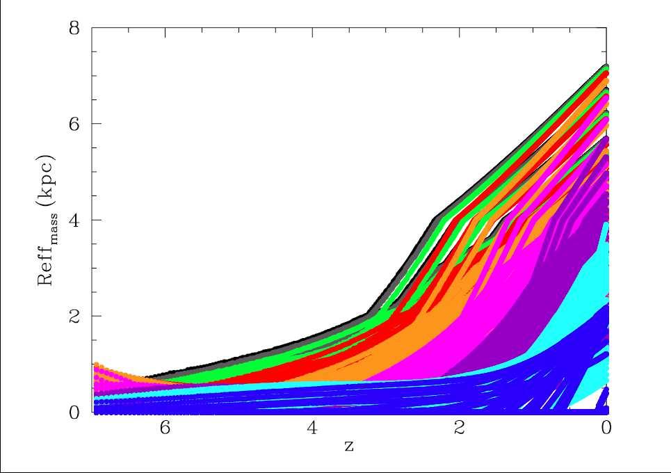
23