LYMAN ALPHA GALAXIES: PHYSICAL PROPERTIES AND EFFECTS OF DUST AT HIGH REDSHIFT. Steven L. Finkelstein

Transcription

1 LYMAN ALPHA GALAXIES: PHYSICAL PROPERTIES AND EFFECTS OF DUST AT HIGH REDSHIFT by Steven L. Finkelstein A Dissertation Presented in Partial Fulfillment of the Requirements for the Degree Doctor of Philosophy ARIZONA STATE UNIVERSITY August 2008

2 c 2008 Steven L. Finkelstein All Rights Reserved

3 LYMAN ALPHA GALAXIES: PHYSICAL PROPERTIES AND EFFECTS OF DUST AT HIGH REDSHIFT by Steven L. Finkelstein has been approved July 2008 Graduate Supervisory Committee: James E. Rhoads, Chair Sangeeta Malhotra Rogier Windhorst Evan Scannapieco John Shumway ACCEPTED BY THE GRADUATE COLLEGE

4 ABSTRACT This dissertation presents the results from five related studies of the nature of Lyman alpha emitting galaxies (LAEs) at high redshifts. These objects have long been predicted to be very young, and possibly the primordial first galaxies. Recent results have shown that these objects may in fact be more complicated. Three different studies at z 4.5 show that LAEs are mostly not primordial, as evidence was found for dust in most of our objects. These studies also show that not all LAEs are young, since two out of a sample of 15 LAEs appear to be much older ( 500 Myr). These older objects are detected with large Lyman alpha equivalent widths (EWs) at an older age due to a clumpy interstellar medium (ISM) geometry. This geometry results in a higher escape fraction for Lyman alpha photons than for continuum photons, thus enhancing the EW to arbitrarily high values. This effect may be responsible for the large number of high EW LAEs detected in recent studies. Extrapolating these stellar population results to the far-infrared (FIR), it appears that nearly half of our sample of LAEs could be detected in their rest-frame FIR with a future observatory such as the Atacama Large Millimeter Array. Detection of the dust emission from these galaxies could confirm the earlier results that many of these objects contain a significant amount of dust. The final study is concerned with LAEs at a much lower redshift of z 0.3. These LAEs are older, more massive, and more metal rich than their high-redshift counterparts, indicating evolution in this type of galaxy. Studying LAEs at low redshift is the highest priority for the future, as one can perform far more detailed analyses then those done at high redshift. iii

5 I dedicate this thesis to my grandfather, Joseph Benezra, the inspiration behind my desire for higher learning. iv

6 ACKNOWLEDGMENTS I would like to acknowledge funding support from the Arizona State University/NASA Space Grant, ASU Department of Physics and ASU School of Earth and Space Exploration. Support for this work was also provided by NASA through grant numbers HST-AR-11249, HST-GO and HST-GO from the Space Telescope Science Institute, which is operated by the Association of Universities for Research in Astronomy, Inc., under NASA contract NAS I would first like to thank my advisor, James Rhoads, for all the help he has given me over the last three years. I am deeply indebted to him for agreeing to take me on as a student before he even set foot at ASU, and for helping me through that first year, where I was knocking on his door nearly every day with some new data reduction problem. I think that the biggest reason for my success is that I always knew that James would take the time to listen to my problem, and offer advice, even when he was busy. Alongside James I would also like to thank Sangeeta Malhotra for all of the great advice, on astronomy and on life, that she has given me. Along with both James and Sangeeta s help, I think the other big reason for my success is that they never stopped pushing me. Be it writing observing proposals, writing grants, or writing an extra chapter for this thesis, I was always urged to do more. While I was not always extremely receptive to these suggestions, in the end I now see that it was for the best, and I thank you both. I also thank my other three committee members, Rogier Windhorst, Evan Scannapieco and John Shumway, v

7 as well as David Smith, for taking the time to read through this thesis and offer valuable suggestions for its improvement. One of the aspects that makes graduate school worthwhile (and tolerable!) are the people you meet, some who just have a passing role in your life, but others who become lifelong friends. Although these people are too many to name here, I would like to especially thank Russell Ryan, Todd Veach, Brian Frank, Allison Loll, Seth Cohen, Nimish Hathi, Amber Straughn, Norman Grogin and Nor Pirzkal for the help you ve given me over the past few years. I would like to thank my parents for their unwavering support. You have been helpful over the years in so many ways, be it listening to me complain about my first year physics courses, to trying to follow along when I explain my research. I don t think I could have finished without your support. To my sisters, Cherie and Elissa, I thank you for at least pretending to be interested when I talk about my research. I also want to thank Jasmine and Bella, for always making me smile. Most importantly, I want to thank my (soon-to-be) wife, Keely. More than anyone else, you have kept me going. This has never been more difficult than over the last year, as we have both been under extreme pressure to finish our schooling. It takes a truly remarkable person to support me in the way that you have, and I am extremely lucky to have you. Very few people have the pleasure of spending their life with someone who shares their same passion, and I feel truly lucky to spend my life with you. vi

8 TABLE OF CONTENTS Page LIST OF FIGURES LIST OF TABLES xii xv CHAPTER 1 INTRODUCTION Present Day Galaxies The First Galaxies Early Detections of Lyman Alpha Galaxies Scientific Results Reasons for Large Lyα EWs Modeling the Stellar Populations of LAEs THE AGES AND MASSES OF Lyα GALAXIES AT z Abstract Introduction Data Handling Observations Data Reduction Lyα Galaxy Selection Stellar Population Models Results Lyα Galaxy Candidates vii

9 CHAPTER Page Equivalent Width Distribution Stacking Analysis Age and Mass Estimates Discussion Age and Mass Estimates Dusty Scenario Conclusions EFFECTS OF DUST GEOMETRY IN Lyα GALAXIES AT z = Abstract Introduction Data Handling Observations Data Reduction Object Extraction Lyα Galaxy Selection Spectroscopic Confirmations Broadband Photometry Modeling Stellar Population Models Dust Effects on the Lyα EW IGM Inhomogeneities viii

10 CHAPTER Page Equivalent Widths Results Fitting to Models Object Object Object Object Best-Fit Models Without Dust Monte Carlo Analysis Discussion Lyα Detection Fraction Hα Equivalent Widths Comparison to Other Work Conclusions Lyα GALAXIES: PRIMITIVE OBJECTS, DUSTY STAR-FORMERS OR EVOLVED GALAXIES? Abstract Introduction Data Handling Observations Object Extraction ix

11 CHAPTER Page Lyα Galaxy Selection Candidate Redshifts Stellar Population Modeling Results Model Fitting NB656 Detected Objects NB665 Detected Objects NB673 Detected Objects Discussion Equivalent Width Distribution Model Parameter Distribution Causes of Model Uncertainties Conclusions THE EXPECTED DETECTION RATE OF DUST EMISSION IN HIGH- REDSHIFT Lyα GALAXIES Abstract Introduction Method Lyα Galaxy Sample Dust Emission Results x

12 CHAPTER Page Lyman Alpha Galaxies Lyman Break Galaxies Robustness of Results Conclusions STELLAR POPULATIONS OF Lyα GALAXIES AT z Abstract Introduction Lyα Galaxy Sample Stellar Population Modeling Results Stellar Population Age and Mass Metallicity, Dust and ISM Clumpiness Stellar Evolution Uncertainties Conclusions CONCLUSIONS REFERENCES xi

13 LIST OF FIGURES Figure Page 1. Distribution of rest-frame Lyman alpha equivalent widths in the LALA Cetus Field Comparison of Cetus Field LAE object stacks to models Comparison of Cetus Field LAE individual detections to models CDF S LAE candidate selection plane Tests for CDF S candidate validity Cut-out stamps of four CDF S LAE candidates Model equivalent width distribution versus stellar population age Best-fit models to four CDF S LAEs Best-fit dust-free models to four CDF S LAEs (a) Results from Monte Carlo simulations for four CDF S LAEs (b) Results from Monte Carlo simulations (continued) Flux selection planes for second CDF S study (a) Cut-out stamps of the new CDF S LAEs (b) Cut-out stamps of the new CDF S LAEs (continued) (a) Best-fit results for all 15 CDF S LAEs (b) Best-fit results for all 15 CDF S LAEs. (continued) (c) Best-fit results for all 15 CDF S LAEs (continued) (d) Best-fit results for all 15 CDF S LAEs (continued) (e) Best-fit results for all 15 CDF S LAEs (continued) xii

14 Figure Page 14. Object and best-fit model equivalent width distributions for all 15 CDF S LAEs Histograms of best-fit results for all CDF S LAEs Histograms of most-likely results for all CDF S LAEs Combined age probability curve averaged over all candidate CDF S LAEs Color-color plane highlighting differences in Lyα and Hα EWs for CDF S LAEs Comparison of LAE and LBG SEDs with ALMA sensitivities Dependence of FIR SED on temperature Color-magnitude diagram for comparing LAEs and LBGs to ALMA sensitivity for z Color-magnitude diagram for comparing LAEs and LBGs to ALMA sensitivity for z Predictions for a z=4.547 millimeter detected starburst galaxy Matching between GALEX positions and broadband images for z 0.3 LAEs (a) Best-fit results for z 0.3 LAEs (b) Best-fit results for z 0.3 LAEs (continued) (c) Best-fit results for z 0.3 LAEs (continued) (d) Best-fit results for z 0.3 LAEs (continued) xiii

15 Figure Page 25. (e) Best-fit results for z 0.3 LAEs (continued) (f) Best-fit results for z 0.3 LAEs (continued) (g) Best-fit results for z 0.3 LAEs (continued) (h) Best-fit results for z 0.3 LAEs (continued) (i) Best-fit results for z 0.3 LAEs (continued) (j) Best-fit results for z 0.3 LAEs (continued) Age distribution for z 0.3 LAEs Mass distribution for z 0.3 LAEs xiv

16 LIST OF TABLES Table Page 1. Best-Fit Ages and Masses for a Constant SFH for Cetus Field LAEs Best-Fit Ages and Masses for an Exponentially Decaying SFH for Cetus Field LAEs CDF S Lyα Galaxy Candidates Magnitudes of CDF S Lyα Galaxy Candidates Maximum Age for a Stellar Population with EW > 200 Å CDF S Best-Fit Physical Parameters Optical Magnitudes of 11 New Lyα Galaxy Candidates NIR and IR Magnitudes of 11 New Lyα Galaxy Candidates Best-Fit Single Population Models for CDF S Lyα Galaxy Candidates Best-Fit Two-Burst Models for CDF S Lyα Galaxy Candidates Derived FIR Properties of LAEs Best-Fit Single Population Models of z 0.3 LAEs xv

17 1. INTRODUCTION 1.1. Present Day Galaxies Studying the formation and evolution of galaxies is currently one of the most active fields in astronomy, vastly helped by the great technological advances over the past few decades. Both large telescopes with multi-ccd cameras as well as big advances in computing power now allow observations and predictions of galaxies in unprecedented detail. In the early 20th century, extra-galactic astronomy focused on the study of nearby objects, as the technology did not exist to probe deeply into the Universe. Initial studies examined the morphology of nearby galaxies, finding that they fell into three main categories which together form the Hubble sequence (Hubble 1936): ellipticals, spirals and irregulars. From their colors, we know that the redder ellipticals are usually passively evolving, with no ongoing star formation (Eggen et al. 1962; Larson & Tinsley 1978). Recent studies suggest that most of these objects are the end result of major galaxy mergers (i.e. Kauffmann & White 1993; Kauffmann et al. 1993). When two galaxies of comparable size collide, it stimulates copious amounts of star formation, using up much of the available star-forming fuel (gas). After a period of time, the galaxy has relaxed into an elliptical shape, and as it is no longer forming stars, its color is redder, reflecting the number of older stars present. Spiral galaxies, on the other hand, contain older stars in a central bulge, with regions of active star formation in a number of outwardly extending spiral arms (e.g., Larson & Tinsley 1978). Gas and dust in these arms get compressed due to spiral density waves, stimulating star formation. Our own Milky Way is a galaxy of this type, and on a dark night one can see the gas and dust fueling this star formation

18 2 as a dark stripe in the Milky Way across the sky. Irregulars come in a variety of shapes, but they are usually less massive than spirals and ellipticals, although they too typically show large amounts of ongoing star formation activity. The vast differences between present day galaxies leads to the natural curiosity of what galaxies looked like in the past. Peering into the history of the universe is possible due to the limitations imposed by the finite speed of light. As we look at more and more distant objects, we are not only looking farther away, but we are also looking back in time, as the photons from these galaxies take time to reach our eyes (or telescopes) at their speed of 300,000 km s 1. This speed is incredibly fast, but it pales in comparison to the vast distances between galaxies. The nearest large spiral to our own is the Andromeda Galaxy (or M31), which at km distant, results in a travel time of 2.5 Myr for its photons to reach the Milky Way. Thus, we are seeing the Andromeda Galaxy as it was 2.5 Myr ago. This technique can be applied to look as far back in time as our current observatories allow. The farther back one wishes to look, the more observing time (or larger telescope) one will need, as flux falls off inversely proportional to the distance squared The First Galaxies Countless studies have been done over the last century peering into the past to examine the history of the Universe. One extremely interesting line of questioning involved the idea of the first galaxies. What did they look like? What kind of stars did they contain? Can we observe them? When did they form? Knowing the redshift of formation was crucial to knowing whether or not these objects could be observed.

19 3 Estimates for the redshift of the first galaxies ranged from 2 z 30 (Djorgovski & Thompson 1992). At these distances, any object would be difficult to observe as the light from objects is spread over an extremely large area. However, Partridge & Peebles (1967) published a study claiming that extremely distant galaxies could be detected. They state that if we are seeing these galaxies during formation, we should expect large bursts of star formation to be occurring, which would create objects with very strong ultraviolet (UV) continua. Nearby, this is difficult to observe from the ground, due to the atmospheric cut-off of UV light. However, in very distant objects, thanks to the expansion of the Universe, the UV light will be redshifted into the optical, which can be observed from the ground. Partridge & Peebles go one step further, stating that as much as 7% of the total radiation could be emitted in a single emission line: Lyman alpha (Lyα). A Lyα photon is emitted when a hydrogen atom transitions from its first excited state into its ground state (2 1). This transition results in the emission of a photon with energy of 10.2 ev, corresponding to a wavelength of Å. Thus, a galaxy with a redshift of 2 will have its Lyα flux detectable from the ground (λ 3700 Å). Strong Lyα emission can be expected from star forming regions. Stars typically form in over-dense regions regions embedded in clouds of molecular hydrogen. When the first massive stars turn on, they will ionize the hydrogen gas out to a certain distance (creating a Strömgren sphere; Strömgren 1939), followed by a region of atomic hydrogen (in what is called the photo-dissociation region), all surrounded by molecular hydrogen. The most massive stars create large numbers of ionizing pho-

20 4 tons, which are photons containing enough energy to ionize a hydrogen atom (E > 13.6 ev; λ < 912 Å). When these photons reach the atomic hydrogen surrounding the star formation region, they will ionize the hydrogen, separating it into component electrons and protons. After a period of time, dependent on the density and temperature, some electrons will recombine with protons, re-forming hydrogen atoms. When they recombine, the electron needs to shed itself of the energy it gained when it was first ionized, and it does this by emitting photons. There are infinite numbers of energy levels which it can transition to in order to rid itself of the unwanted energy, but hydrogen atoms typically follow a few de-excitation paths, many of which involve the emission of a Lyα photon at the end. In fact, using case B recombination assumptions (which assumes that every Lyman-line photon undergoes many scatterings, also known as the large optical depth approximation), when a hydrogen atom recombines, there is a 2/3 chance that it will emit a Lyα photon to move it into the ground state. Thus, strong star formation begets many ionizing photons, which beget many Lyα photons, which explains the prediction of Partridge & Peebles. This prediction spawned a plethora of studies to find the first galaxies (e.g., Meier & Terlevich 1981; Koo & Kron 1980; Djorgovski & Thompson 1992; De Propris et al. 1993; Cowie & Hu 1998; Rhoads et al. 2000). Standard theories predicted that they would be primeval in nature. That is, their metallicities would be extremely low, as metals require previous generations of stars. We could also expect there to be no dust present, assuming that the observations take place before the first stars begin to die. They could also contain the not-yet-detected metal-free stars, known as

21 5 Population III stars. Most of these first studies met with failure, as, though they used a wide variety of methods to detect redshifted Lyα emission lines, they were unable to confirm detection of the expected population of primeval galaxies (e.g., Koo & Kron 1980; Djorgovski & Thompson 1992; De Propris et al. 1993). Djorgovski & Thompson (1992) predicted that these objects should have an expected Lyα line flux of erg s 1 cm 2, which they claimed to be observable with their present day technology. When no candidate primeval galaxies (or Lyα galaxies as we shall call them from here on) were found, numerous ideas were presented to explain their scarcity. Perhaps their fluxes were less than predicted, possibly due to dust (Meier & Terlevich 1981). Lyα photons are resonantly scattered by neutral hydrogen, meaning that they effectively bounce off as they are absorbed and re-emitted, although they can be re-emitted in any direction. Thus, in a homogeneous medium, Lyα photons have much longer path lengths than continuum photons, strongly increasing their chance of encountering a dust grain if dust is present. Add that to the fact that Lyα photons have a much greater chance of absorption than redder continuum photons, and one can begin to see how a small amount of dust could vastly extinguish Lyα flux. This idea had its flaws, as Lyα galaxies (or Lyα emitting galaxies; LAEs) were supposed to be primitive, containing no dust. Nonetheless, this issue remained unresolved until the late 1990 s, when two groups (Cowie & Hu 1998 & Rhoads et al. 2000) detected the first large samples of field LAEs.

22 Early Detections of Lyman Alpha Galaxies There are three popular techniques for locating high-redshift galaxies. The first is called the Lyman break technique, pioneered by Steidel et al. (1996). This method involves observing a patch of sky in two adjacent broadband filters, such that the Lyα line falls roughly in the filter overlap region. Flux blueward of the Lyα line suffers attenuation due to clumps of neutral hydrogen in the intergalactic medium (IGM), thus even an object with a flat intrinsic continuum will show a red color between these filters. A color criterion can thus be determined to select galaxies at the chosen redshift with a z range of 1. Follow-up spectroscopy can then confirm the redshift estimate, as well as measure a Lyα emission line if one is present (e.g., Shapley 2001, 2003). This method has the benefit of finding large numbers of highredshift galaxies, but the detriment that follow-up spectroscopy is needed to further confirm the redshift and to measure the Lyα flux. The second technique involves using a random mask of slits to perform a blind spectroscopic search for LAEs in a typically blank field (e.g., Martin et al. 2008). This has an advantage over the Lyman break technique in that one obtains the redshift and Lyα line flux in one (usually deeper) observation, but this technique necessitates serendipitous slit placement, and thus the number of objects detected is much less. The third method, narrowband selection, is one of the most popular techniques. One observes a blank field in a narrowband and a broadband filter, with the narrowband residing approximately in the middle of the broadband wavelength coverage. One then compares sources in the two images, and if a source is brighter in the narrowband

23 7 than in the broadband, it is an emission line galaxy candidate. This method covers the same angular area as the Lyman break technique, but samples a much thinner slice of redshift space, with a typical z 0.1. While this reduces the total number of objects selected, it gives one a much better estimate of the object s redshift (although typically follow-up spectroscopy is desired to pinpoint the redshift, and confirm that the object is indeed a LAE). Cowie and Hu (1998) used the narrowband selection technique to locate a sample of 10 LAEs at z 3.4 down to a Lyα line flux of erg s 1 cm 2 over 46 arcmin 2. Rhoads et al. (2000) started the Large Area Lyman Alpha survey (LALA), which in this first paper published the finding of 174 LAEs at z 4.5 in two adjacent narrowband filters over 0.3 deg 2, with narrowband fluxes from 2.6 to erg s 1 cm 2. Why did these two surveys succeed when surveys not five years earlier failed? The answers are different, but the underlying cause is the same: technological advancement. Cowie and Hu made use of the Keck telescopes for their observations, which with 10m diameter mirrors, are the largest telescopes in the world (at the time of this writing). Keck came online in the mid-1990 s, thus it was not available for the earlier studies. Cowie and Hu were able to probe fainter line fluxes, close to erg s 1 cm 2, resulting in their discovery of numerous LAEs, even though their instrument (LRIS) had a field-of-view comparable to that used by Djorgovski & Thompson ( 5 arcmin 2 ; 1992). While the LALA survey used the 4 m Mayall telescope at the Kitt Peak National Observatory, which had been around for decades, they made use of the very new

24 8 MOSAIC camera, which allowed observations over a wide field by pasting together eight 2048x4096 CCDs, for a field-of-view of 1296 arcmin 2 (or 0.36 deg 2 ). This field of view is over 200 times larger than that used by Djorgovski & Thompson (1992), thus Rhoads et al. were able to detect large numbers of candidate LAEs in only 6 hours of imaging per filter. We can thus see that Lyα galaxies were fainter and sparser than originally predicted, as Cowie & Hu and Rhoads et al. have shown that an increase in depth and/or field-of-view results in the successful discovery of large numbers of LAEs Scientific Results In the few years following these first detections there were numerous topics for study, as including the Lyα equivalent widths (e.g., Malhotra & Rhoads 2002, hereafter MR02; Dawson et al. 2007) and the Lyα luminosity functions (e.g., Malhotra & Rhoads 2004; Dawson et al. 2004, 2007; Gronwall et al. 2007; Ouchi et al. 2008; Deharveng et al. 2008). The luminosity function studies primarily looked into the evolution of the luminosity function with redshift to search for changes in LAE number density. Finding evidence that the LAE number density decreases at higher redshift could indicate that the IGM is becoming predominantly more neutral, and as thus is evidence for the onset of reionization. The results from these studies are still ambiguous, although both Malhotra & Rhoads (2004) and Ouchi et al. (2008) found results consistent with no evolution out to z 6.5, implying that their observations have not yet located the epoch of reionization. Deharveng et al. (2008) published a luminosity function for LAEs at z 0.3, identified using the Galaxy Evolution Explorer

25 9 (GALEX), finding that the number densities of LAEs at z 0.3 is much less than that at z 3.1 (Gronwall et al. 2007), implying significant evolution towards lower redshifts, perhaps consistent with hierarchical clustering theories of galaxy evolution. In a spectroscopic study, Dawson et al. (2007) found that a non-negligible fraction of their confirmed Lyα lines had rest-frame equivalent widths (EWs) exceeding theoretical predictions from normal stellar populations. A stellar population with solar metallicity, a Salpeter (1955) initial mass function (IMF) and a constant star formation history will have a maximum Lyα EW of 260 Å at 1 Myr, dropping rapidly to a constant value of 95 Å by 100 Myr (dropping to zero in any kind of decaying star formation history). Dawson et al. found that 12 27% of their LAEs showed rest-frame EWs > 240 Å. They were not the first to see this, as both Kudritzki et al. (2000) and MR02 also found a large number of LAEs with strong EWs. While it is certainly possible for a single LAE to have an EW near 250 Å, the sheer number of high EW objects indicates that either a large fraction of LAEs are 1 Myr, or that our initial assumptions are wrong. It is exceedingly unlikely that a large fraction of LAEs are only 1 Myr old, and even if they were, the chance that we would observe them during that 1 Myr is small Reasons for Large Lyα EWs There are a few possibilities which could explain the large EWs seen in LAEs. The first possibility is that these objects are creating more ionizing photons than we know of, which in turn creates more Lyα photons. This could happen if the metallicity was extremely low, which would create hot stars. If the metallicity was zero, Popula-

26 10 tion III stars could be created. These zero metallicity objects would be expected to produce regions with very large Lyα EWs (Scannapeico et al. 2003; Venkatesan et al. 2003). Due to their hard spectra, these objects produce many photons which are capable of ionizing Heii, thus Heii recombination lines, such as λ1640, λ3202 and λ4686, could be possible signatures of Population III stars (i.e., Tumlinson & Shull 2000; Tumlinson et al. 2001). However, these signatures (specifically the 1640 Å line, which is expected to be the strongest; Tumlinson et al. 2001) have yet to be definitively detected (e.g., Dawson et al. 2004; Nagao et al. 2008), casting doubt upon the existence of Population III stars in these objects. Even a near zero metallicity will result in some increase in the Lyα line strength through hotter photospheres and/or top-heavy IMFs (e.g., Schaerer 2002; Schneider et al. 2006), although whether it is enough to explain the observations is doubtful. Active galactic nuclei (AGN) are extremely bright regions near the centers of many galaxies which are fueled by the central black holes in these galaxies. AGN typically show an assortment of high ionization state emission lines, as well as a very strong Lyα line. These Lyα photons are not produced by star formation, and thus there is no fiducial limit on the EW. Thus, to be sure that known LAEs are not AGN, we have to screen against them. This is typically done in two ways. First, AGN frequently emit in X-rays, thus if a LAE is X-ray detected, it is a sign that it is a possible AGN. Wang et al. (2004) and Malhotra et al. (2003) surveyed Chandra X-ray data of the LALA fields, and concluded that less than 4.8% of the LAEs they studied could be possible AGN. However, in some cases it is possible that the X-rays

27 11 can be obscured, and thus it is also prudent to obtain spectra and check for the typical high ionization state lines seen in AGN. Dawson et al. (2004) found no detection of these lines in LAEs from the LALA survey, providing further proof that the majority of narrowband selected LAEs are not AGN, thus an active galactic nucleus is an unlikely source for the stronger than expected EWs observed. Another possible cause of large Lyα EWs in high-redshift LAEs involves dust. According to Meier and Terlevich (1981), dust should severely attenuate Lyα, even more than continuum light, resulting in lower EWs. However, this involves an assumption that the interstellar medium (ISM) is roughly uniform, meaning that the Lyα will see dust in every direction. However, what if the ISM was clumpy? Neufeld (1991) argued (and Haiman & Spaans 1999 and Hansen & Oh 2006 theoretically confirmed) that if the ISM was sufficiently clumpy, the opposite effect could actually occur. Imagine an ISM consisting of clumps of evenly mixed dust and neutral hydrogen, with the inter-clump medium only containing ionized hydrogen. A Lyα photon will move freely throughout this ISM until it encounters a clump. When it does encounter a clump, it will be resonantly scattered by a hydrogen atom at the surface. At this point, it will be re-emitted in any direction, meaning that 50% of the time, it will move back out into the inter-clump medium. Even if it is sent directly into the clump, it will be absorbed immediately by the next hydrogen atom it encounters, thus it is extremely difficult for Lyα photons to penetrate deeply into these clumps. Continuum photons suffer no such restrictions. They are not resonantly scattered by hydrogen, and thus they will make their way deeper into a clump, until they

28 12 are eventually absorbed or scattered by a dust grain, resulting in extinction and/or reddening of the continuum light. Thus, this ISM geometry results in (most of) the Lyα photons being screened from ever encountering a dust grain. Since the EW is a measure of the Lyα to continuum ratio, the EW we would measure is increased relative to the intrinsic value coming out of the star formation regions. While this scenario posed a definite possible explanation for the observed EW distribution, we had no way to study its existence until recently Modeling the Stellar Populations of LAEs The technique of learning about distant galaxies by comparing their observed spectral energy distributions (SEDs) to theoretical models has gained popularity in recent years. The most widely used models are those of Bruzual & Charlot (2003; BC03). Essentially, these models take as input a stellar population metallicity, star formation history and age, and output the combined spectrum of all of the stars. One then fits a grid of models to their observations in order to see which model best explains the observed SED. Over the past five years, a few groups have used this technique to learn about Lyα galaxies (Chary et al. 2005; Gawiser et al. 2006; Pirzkal et al. 2007; Lai et al. 2007, 2008; Nilsson et al. 2007). Most of these studies find that LAEs are in general young and low mass, consistent with earlier predictions. One thing these studies lack is a detailed examination of the contribution of the Lyα line to the SED. The motivation behind this thesis is to improve upon these earlier studies in order to investigate the cause of the large number of high EW LAEs seen. To do this we compare observations to models which include the effect of not

29 13 only a Lyα emission line, but also the effect of dust geometry (or clumpiness) on the Lyα EW. While the BC03 models do not tabulate emission line strengths, they do give the number of ionizing photons present in a given stellar population, which (using case B recombination assumptions) one can convert into a Lyα flux. In Chapter 2 we discuss our first study, where we obtained continuum measurements of LAEs via broadband imaging. These ground-based observations were not deep enough to constrain the dusty scenario, but we were able to confirm that those LAEs with the largest Lyα EWs were (on average) some of the youngest and lowest mass objects in the Universe known to date. In Chapter 3, we improve upon our previous work by obtaining narrowband observations in the Great Observatories Origins Deep Survey (GOODS) Chandra Deep Field South (CDF S), which allowed the discovery of four new LAEs in a field with very deep public space-based broadband data. These deeper data allowed us to fit stellar population models to individual LAEs. Chapter 4 continues the work of Chapter 3 with a much larger sample of LAEs. In Chapter 5, we discuss different ways of constraining the dust in these objects by studying the likelihood of detecting dust emission from high-redshift LAEs. In Chapter 6, we finish with an analysis of low-redshift LAEs, and discuss the differences from their high-redshift counterparts. In Chapter 7, we present our conclusions, drawing upon the results of each study. Chapters 2 and 3 are published in the Astrophysical Journal, volume 660, page 1023 and volume 678, page 655 respectively. At the time of this writing, Chapter 4 is undergoing peer review at the Astrophysical Journal, Chapter 5 is undergoing peer review at the Monthly Notices

30 14 of the Royal Astronomical Society, and Chapter 6 is in preparation for submission to the Astrophysical Journal.

31 2. THE AGES AND MASSES OF Lyα GALAXIES AT z Abstract We examine the stellar populations of a sample of 98 z 4.5 Lyα emitting galaxies using their broadband colors derived from deep photometry at the Multiple Mirror Telescope (MMT). These galaxies were selected by narrowband excess from the Large Area Lyman Alpha survey. Twenty-two galaxies are detected in two or more of our MMT filters (g, r, i and z ), with calculated rest-frame equivalent widths (EWs) from 5 to 800 Å. By comparing broad and narrowband colors of these galaxies to synthetic colors from stellar population models, we determine their ages and stellar masses. The highest EW objects have an average age of 4 Myr, consistent with ongoing star formation. The lowest EW objects show an age of Myr, consistent with the expectation that larger numbers of older stars are causing low EWs. We found stellar masses ranging from M for the youngest objects in the sample to M for the oldest. It is possible that dust effects could produce large EWs even in older populations by allowing the Lyα photons to escape, even while the continuum is extinguished, and we also present models for this scenario Introduction There are two popular techniques for locating galaxies at high redshift: the Lyman break technique (Steidel et al. 1996) and narrowband selection. The latter entails observing a galaxy in a narrowband filter containing a redshifted emission line. This method is useful to select high-redshift galaxies with strong Lyman alpha (Lyα) emission lines. While the line emission properties of Lyman break galaxies (LBGs) are known, little is known about the continuum properties of Lyα galaxies because they are so faint. Studying the continuum properties of these Lyα galaxies at high

32 16 redshift can tell us about their age, stellar mass, dust content and star formation history. We have used the narrowband selection technique to locate and study Lyα emitting galaxies (LAEs) in the Large Area Lyman Alpha (LALA; Rhoads et al. 2000) survey Cetus Field at z 4.5. Similar studies have been done both in this field and in other fields (e.g., Rhoads et al. 2000, 2004; Rhoads & Malhotra 2001; Malhotra & Rhoads 2002; Cowie & Hu 1998; Hu et al. 1998, 2002, 2004; Kudritzki et al 2000; Fynbo, Möller, & Thomsen 2001; Pentericci et al. 2000; Stiavelli et al. 2001; Ouchi et al. 2001, 2003, 2004; Fujita et al. 2003; Shimasaku et al. 2003, 2006; Kodaira et al. 2003; Ajiki et al. 2004; Taniguchi et al. 2005; Venemans et al. 2002, 2004; Pascarelle et al. 1996ab). In many of these studies, the strength of the Lyα line has been found to be much greater than that of a normal stellar population (Kudritzki et al. 2000; Dawson et al. 2004). Malhotra & Rhoads (2002, hereafter MR02) found numerous LAEs with rest-frame equivalent widths (EWs) > 200 Å. Assuming a constant star formation history, the EW of a normal stellar population will asymptote toward 80 Å by 10 8 yr, down from a maximum value of 240 Å. These galaxies are of interest, because it is believed that this strong Lyα emission is a sign of ongoing star formation activity in these galaxies (Partridge & Peebles 1967), and it could mean that these are some of the youngest galaxies in the early universe. There are a few possible scenarios that could be creating these large EWs. Strong Lyα emission could be produced via star formation if the stellar photospheres are hotter than normal, which could happen in low-metallicity galaxies. It could also

33 17 mean that these galaxies have their stellar mass distributed via a top-heavy initial mass function (IMF). Both of these scenarios are possible in primitive galaxies, which are thought to contain young stars and little dust. Active galactic nuclei (AGNs) can also produce large Lyα EWs. In an optical spectroscopic survey of z 4.5 Lyα galaxies, Dawson et al. (2004) found large Lyα EWs, but narrow physical widths ( v < 500 km s 1 ). They placed tight upper limits on the flux of accompanying high-ionization state emission lines (e.g., Nv λ1240, Siiv λ1398, Civ λ1549 and Heii λ1640), suggesting that the large Lyα EWs are powered by star formation rather than AGNs. Type I (broad-lined) AGNs are also ruled out as the Lyα line width is greater than the width of the used narrowband filters. While Type II AGN lines are narrower than our filters, they remain broader than the typical line width of our Lyα sample as determined by follow-up spectroscopy (e.g., Rhoads et al. 2003). Malhotra et al. (2003) and Wang et al. (2004) searched for a correlation between LAEs and Type II AGNs using deep Chandra X-Ray Observatory images. None of the 101 Lyα emitters known to lie in the two fields observed with Chandra were detected at the 3 σ level (L 2 8keV = erg s 1 ). The sources remained undetected when they were stacked, and they concluded that less than 4.8% of the Lyα emitters they studied could be possible AGNs. Therefore, we are confident that there are at most a few AGNs in our Lyα galaxy sample. Another possible scenario involves enhancement of the Lyα EW in a clumpy medium. In this scenario, the continuum light is attenuated by dust, whereas the Lyα line is not, resulting in a greatly enhanced observed Lyα EW (Neufeld 1991;

34 18 Hansen & Oh 2006). This can happen if the dust is primarily in cold, neutral clouds, whereas the inter-cloud medium is hot and mainly ionized. Because Lyα photons are resonantly scattered, they are preferentially absorbed at the surface. Thus, it is highly unlikely that a Lyα photon will penetrate deep into one of these clouds. They will be absorbed and re-emitted right at the surface, effectively scattering off of the clouds and spending the majority of their time in the inter-cloud medium. However, continuum photons are not resonantly scattered, and if the covering factor of clouds is large, they will in general pass through the interior of one. Thus the continuum photons will suffer greater attenuation than the Lyα photons, effectively enhancing the Lyα EW. These Lyα galaxies are so faint compared to other high-z objects that have been studied, that not a lot is known about their continuum properties. Our primary goal is to better constrain the ages and stellar masses of these objects from their continuum light in order to better understand the driving force behind the strength of the Lyα line. We have obtained deep broadband imaging in the g, r, i and z bands for this purpose. Using the colors of these galaxies, we can study continuum properties of individual Lyα emitting galaxies at this redshift for the first time, allowing us to estimate their age, mass, star formation history and dust content. The next phase of our project will be to look into the likelihood of dust causing the large Lyα EW, which we will begin to do in this paper, as the colors of these galaxies might distinguish the cause of the large EW. Blue colors would indicate young stars with hot photospheres, while red colors would indicate dust quenching of the continuum,

35 19 enhancing the Lyα EW. Observations, data reduction technique and sample selection are reported in 2.3; results are presented in 2.4, and they are discussed in 2.5. Conclusions are presented in Data Handling Observations The LALA survey began in 1998 using the 4m Mayall telescope at the Kitt Peak National Observatory (KPNO). The final area of this survey was 0.72 deg 2 in two fields, Boötes and Cetus, centered at 14:25:57, +35:32:00 (J2000.0) and 02:05:20, -04:55:00 (J2000.0), respectively (Rhoads et al. 2000). The LALA survey found large samples of Lyα emitting galaxies at z = 4.5, 5.7, and 6.5, with a spectroscopic success rate of up to 70%. We observed the LALA Cetus Field for three full nights in November 2005, and again for four 1 4 nights in January 2006, using the Megacam instrument (McLeod et al. 1998) at the Multiple Mirror Telescope (MMT). Megacam is a large mosaic charge-coupled device (CCD) camera with a field of view, made up of pixel CCDs. Each pixel is 0.08 on the sky. We acquired deep broadband images in four Sloan Digital Sky Survey (SDSS) filters: g (λ c 4750 Å), r ( 6250 Å), i ( 7750 Å) and z ( 9100 Å). The total exposure time in the g, r, i, and z filters were 4.33, 3.50, 4.78 and 5.33 hr, respectively. Given that the seeing during the run was rarely below 0.8, we chose to bin the pixels 2 2 to reduce data volume, resulting in a final pixel scale of 0.16 pixel 1 in our individual images.

36 Data Reduction The data were reduced in IRAF 1 (Tody 1986, 1993), using the MSCRED (Valdes & Tody 1998; Valdes 1998) and MEGARED (McLeod et al. 2006) reduction packages. The data were first processed using the standard CCD reduction steps done by the task ccdproc (overscan correction, trim, bias subtraction and flat fielding). Bad pixels were flagged using the Megacam bad pixel masks included with the MEGARED package. Fringing was present in the i - and z -band data, and needed to be removed. For this, we made object masks using the task objmasks. 2 We then took a set of science frames in each filter, and combined them to make a skyflat using sflatcombine (using the object masks to exclude any objects from the resulting image). This skyflat was then median smoothed on a scale of pixels (i ) and pixels (z ). The smoothed images were subtracted from the unsmoothed images, and the result was a fringe frame for each band. The fringing was then removed from the science images using the task rmfringe, which scales and subtracts the fringe frame. To make the illumination correction, skyflats were made, median smoothed 5 5 pixels, normalized, and divided out of the science images. The amplifiers in the reduced images were merged (from 72 to 36 extensions) using the MEGARED task megamerge. The World Coordinate System (WCS) writ- 1 IRAF is distributed by the National Optical Astronomy Observatory (NOAO), which is operated by the Association of Universities for Research in Astronomy, Inc. (AURA), under cooperative agreement with the National Science Foundation. 2 In order to prevent fringing from making it onto the object masks, we first made a skyflat without object masks, and divided this skyflat out of the science data. We then got the object masks from these quasi-fringe removed images. The rest of the procedure used the untouched science frames.

37 21 ten in the image header at the telescope is systematically off by 0.5 in rotation, so we used the task fixmosaic to adjust the rotation angle so that the WCS solution works better. The WCS was then determined using megawcs, and the WCS distortion terms were installed in the header using the task zpn. The 36 chips were combined into a single extension using the program SWarp 3. We ran SWarp on each input image, using a corresponding weight map that gave zero weight to known bad pixels and cosmic-ray hits. We located the cosmic rays using the method of Rhoads (2000). We specified the center of the output images to be the average center of the five dither positions we used (02:04:56, -05:01:01 [J2000.0]), which corresponded to an image size of pixels and a pixel scale of pixel 1. During this process, each image was resampled (using the Lanczos-3 6-tap filter) and interpolated onto the new pixel grid. While this was done, SWarp determined and subtracted the background value in each extension. An initial stack for each filter was made using SWarp to average together the individual images. To make the final version of the stack, we needed to remove the satellite trails that littered our images. To do this, we created a difference image between each individual input image and the initial stack. Using a thresholding technique, we flagged the satellite trails in this image, and combined those flags with the existing weight maps. We ran SWarp a final time with this as the input weight map, creating the final stack. We did this process for each band, giving us four images, one final stack in each of the g, r, i and z bands. In an attempt to increase 3 SWarp is a program that resamples and co-adds together FITS images, authored by Emmanuel Bertin. It is distributed by Terapix at

38 22 the signal of our objects, we tried co-adding R- and I-band images from the NOAO Deep Wide-Field Survey (NDWFS; Jannuzi & Dey 1999) to our r and i images; however, the additional signal did not make a significant difference in the results. The median FWHM in the final stacks were: g =1.29, r =1.08, i =1.25 and z =1.32. To calculate the photometric zero point for our observations we took images of the standard stars SA and SA during our run, where the zeropoint is defined as the magnitude of an object with one count in the image (for an integration time of 400 s). These standard stars are from Landolt (1992), and we used the transforms from Johnson-Morgan-Cousins to SDSS magnitudes from Fukugita et al. (1996). Averaging the results from the two stars for each band, we obtained these zero points: g =33.13, r =33.00, i =32.58 and z =31.43 mag. Using these zero points with our data, all of our results are in AB magnitudes Lyα Galaxy Selection To extract the objects from each stack, we used the SExtractor package (Bertin & Arnouts, 1996). For SExtractor to accurately estimate the errors in the flux, it needed to know the gain in the input images. To calculate this, we needed the mean and standard deviation of the background of the images. Because the background was subtracted out in SWarp, we obtained the average background value in each band by averaging the values obtained from the pre-swarped images, and adding this value onto the final stacks. We then ran SExtractor in the two-image mode using a 9 pixel aperture (2.32 ) with the narrowband images from the LALA survey, giving us catalogs of objects that were detected in both images.

39 23 To calculate the errors on our photometry, we measured aperture fluxes at a few million randomly placed locations throughout the image. We performed the aperture photometry using SExtractor in two-image mode, with our stacked images as the photometry image and an artificial image containing randomly placed points as the detection image. We then measured σ empirically from the distribution of counts in these random apertures. The 5σ limiting magnitudes of our final stacks, measured in 2.32 diameter (9 pixel) apertures, were g =26.38, r =25.64, i =25.13 and z =24.31 mag. The method we have used to locate Lyα galaxies involves taking an image using a narrowband filter containing the wavelength for Lyα at a certain redshift. We used the catalog from MR02, which was based on LALA narrowband images and broadband B w, R, and I data from the NDWFS (Jannuzi & Dey 1999). The narrowband data consist of five overlapping narrowband filters, each with a FWHM 80 Å. The central wavelengths are λλ6559 (H0), 6611 (H4), 6650 (H8), 6692 (H12), and 6730 (H16), giving a total redshift coverage 4.37 < z < To ensure that there was no overlap, we only used objects selected from the H0, H8 and H16 filters in our analysis. In order to compare the two data sets, the Megacam data were registered and remapped onto the same scale as the narrowband data using the IRAF tasks wcsmap and geotran. Selection criteria for the MR02 catalog, following Rhoads & Malhotra (2001), were as follows: (1) 5 σ significance detection in the narrowband. This is calculated using an SExtractor aperture flux with the associated flux error; flux/error 5. (2)

40 24 4 σ significant excess of narrowband flux. This was calculated by taking narrowband flux broadband flux, both calibrated in physical units, and the associated error [sqrt(error 2 broad + error 2 narrow)] and demanding that flux difference / error 4. (3) Factor of 2 ratio between broad and narrowband fluxes, calibrated to the same units. (4) No more than 2 σ significant flux in the bluest filter observed (B w ) Stellar Population Models In order to study the properties of the galaxies in our sample we compare them to stellar population models, using the stellar population modeling software of Bruzual & Charlot (2003). With these models, we were able to choose a range of ages, metallicities and star formation histories for comparison with our sample. We chose ages ranging from 10 6 to 10 9 yr, metallicities from 0.02 Z to Z and exponentially decaying star formation histories with a characteristic timescale of τ = yr. We included dust via the Calzetti dust extinction law (Calzetti et al. 1994), which is applicable to starburst galaxies, in the range A 1200 = 0-2 mag. Finally, we included intergalactic medium (IGM) absorption via the prescription of Madau (1995). The Bruzual & Charlot (2003, hereafter BC03) code output the flux of a given stellar population in units of L Å 1. In order to go from flux in these units to bandpass averaged fluxes, we used the method outlined by Papovich et al. (2001). In short, we took the output from BC03, and converted it from L λ into L ν, and then from L ν into F ν (in units of ergs s 1 cm 2 Hz 1 ) using F ν = (1 + z) L ν / (4πd 2 L). This flux was then multiplied by the transmission function for a given bandpass, and integrated over all frequency. The bandpass averaged flux f ν is this result normalized to the

41 25 integral of the transmission function. AB magnitudes (Oke & Gunn, 1983) for the candidates were then computed. In order to calculate colors that we could directly compare to our observations, it was necessary to add in emission-line flux from the Lyα line, which appears in the r filter at z 4.5. While the BC03 software does not calculate emission-line strengths, we were able to use one of its many other output quantities: the number of ionizing photons. We calculated the Lyα emission-line strength 4 (in units of L Å 1 to match the model output) by using Lyα Linestrength = hc λ Lyα L λ 2 3 n ion (1) where n ion is the number of ionizing photons, λ is the bin size of the wavelength array (1 Å), and the factor of 2/3 represents the fraction of ionizing photons that will produce Lyα photons when interacting with the local interstellar medium (ISM) under case B recombination. In effect, this spreads the line flux over a finite wavelength interval, so that the conversion from L ν to F ν properly redshifts both the line and continuum emission. In order to model the clumpy dust scenario, we needed to ensure that the Lyα line did not suffer dust attenuation. To do this, the continuum flux was multiplied by the Calzetti dust law before we added in the Lyα flux to the spectrum at the correct wavelength bin. In this case, the continuum suffers dust attenuation, while the Lyα line does not. 4 This calculation follows the simple assumptions that no ionizing photons escape, and that all Lyα photons escape.

42 Results Lyα Galaxy Candidates Using the catalog described above, we have identified 98 objects as Lyα galaxy candidates within the Megacam field of view, in a total comoving volume of Mpc 3 (using the three non-overlapping LALA narrowband filters). We have classified 22 of these objects as continuum detections on the basis that they have at least 2σ detections in two of the r, i, or z bands (the other 76 objects were undetected at this level in the broadband data, but we later stacked their fluxes for analysis). We have in our possession Inamori Magellan Areal Camera and Spectrograph (IMACS) spectra of objects in the LALA Cetus Field (Wang et al. 2007). These spectra have been used to identify the redshift of the Lyα line in these galaxies. Out of the 98 total Lyα galaxy candidates, 28 have been spectroscopically confirmed as being Lyα emitters at z 4.5. Seven of these confirmations are among the 22 Megacam detections. Another seven of the Megacam detections have IMACS spectra but had no strong Lyα line identified. However, some of these may show a line with deeper spectra Equivalent Width Distribution We calculated the rest-frame equivalent widths of our 22 detections using the ratio of the line flux to the continuum flux via EW = ( 1 η η λ BB 1 λ NB ) (1 + z) 1 (2)

43 27 where η is the ratio of narrowband to broadband flux (in units of f ν ), and λ are the filter widths (80 and 1220 Å for the narrow and broad filters, respectively). The narrowband fluxes are measured from the LALA narrowband data discussed above, and the broadband fluxes are measured from our MMT r data. Figure 1 shows the calculated rest-frame EWs of our 22 continuum-detected galaxies. The range of EWs is Å. 5 While the range of our EW distribution peaks at the low end of previous studies (i.e. most of our objects have rest-frame EW 200 Å), we recognize that the 76 undetected objects would all lie at the high EW end of this plot (in fact, they peak at EW well over 200 Å). Because they are undetected, this means that their broadband fluxes were too faint to be detected in our survey. However, they still have very bright narrowband fluxes, indicating strong Lyα emission. This strong emission, coupled with faint broadband r magnitudes, results in a high Lyα EW. From models of normal stellar populations (those with a near-solar metallicity and a Salpeter (1955) IMF), it was found that the maximum EW a galaxy could have is 240 Å at t 10 6 yr, with the EW approaching a steady value of 80 Å at t 10 8 yr (MR02; Charlot & Fall 1993). Our data show many objects with a rest-frame EW greater than 100 Å. While individual galaxies with EWs this high are possible from normal stellar populations, the ratio of high-low EWs is much greater than it ought to be when we account for the 76 objects without MMT detections. This implies that something is causing the EWs to be higher than normal. MR02 consider several 5 However, the object with an EW of 5 Å is likely an interloper. It has a 10 σ detection in g, and > 30 σ detections in r, i and z. We exclude this object from the rest of our analysis, giving us 21 detections.

44 28 possible explanations for this observation. Hot photospheres and/or the radiative transfer effects discussed above are sufficient explanations. Another possibility is that galaxies above a certain age, around 10 8 yr, are removed from the sample by some mechanism. For example, the first generations of stars might form (uniformly distributed) dust that further suppresses the Lyα EW, removing a large proportion of intermediate-ew objects from the sample. One of our goals in this study is to investigate whether the cause is massive stars creating more Lyα photons, or dust suppressing the continuum and thus enhancing the Lyα EW. We note that four objects among our MMT detections show rest-frame EWs in excess of 230 Å. Such high EWs might be explained by a combination of extreme youth and/or low metallicity (e.g. Malhotra & Rhoads 2004), or might be produced by radiative transfer effects (Neufeld 1991; Hansen & Oh 2006). However, two of these objects are consistent with 200 Å EW at the 1 σ level, and the other two at the 2 σ level, so such mechanisms are not strictly required to explain these objects. Stronger evidence for such effects may be found among the 76 sources whose continuum emission was too faint for our MMT data Stacking Analysis Our goal has been to be able to compare our objects to the models to obtain estimates of physical parameters such as age and stellar mass, along with dust content. We divided our objects into six groups that we then stacked (in order to increase the signal to noise) to get composite fluxes that we could compare to the models. The groups are: non-detections, which consists of the 76 selected objects which did not

45 FIG. 1. Distribution of rest-frame Lyα EWs from our 22 detections. The EWs range from 5 to 800 Å. The single object with EW < 20 Å is likely an interloper that has managed to satisfy our selection criteria. A normal stellar population has an EW that asymptotes to 80 Å as its age goes to 10 8 yr, so something is causing the Lyα EW of many of these objects to be higher. 29

46 30 have a 2 σ detection in at least two bands (out of r, i, and z ); low EW, which consists of the seven detected objects with EW of Å; middle EW, which consists of the seven detected objects with EW of Å; high EW, which consists of the seven detected objects with EW 110 Å; detections, which consists of the 21 objects that were detected in the Megacam data; spectroscopically confirmed, which consists of the 28 objects (seven detected) that were confirmed to be Lyα emitters at z 4.5. These stacks are shown in Figure Age and Mass Estimates In order to study these galaxies, we have created numerous synthetic stellar population models that we compare to our observed galaxies. The most illuminating way in which we can study the observed vs. model galaxies are in color-color plots (Figure 2 and Figure 3). We have plotted the r - nb color vs. the r - i color of our objects, and then overplotted various model curves. Because changing the metallicity did not much change the position of the model curves in the plane we are studying, we have elected to only use models with Z =.02 Z. The differing line styles represent the two different star formation histories we used, with the solid lines representing continuous star formation, and the dashed lines representing exponentially decaying star formation with a decay time of τ = 10 7 yr. We ran the models at 24 different ages ranging from 1 Myr to 2 Gyr, 6 and in the figure we show the five ages that best surround the data, represented by different colors. We included dust in the models, ranging from A 1200 = 0 to 2. The extent of 6 At 1 Myr, the two different star formation histories have identical colors, so their model tracks overlap, that is why it appears as if there is no curve for an exponentially decaying galaxy at 1 Myr.

47 31 the model tracks represents the different dust optical depths. As we discussed above, this dust does not affect the strength of the model Lyα line. We have connected the zero-dust end of the model tracks with the dotted black line in order to show where galaxies with no dust should lie. With significant flux in only three broadband points (r, i, and z ), it would be hard to fit each stack to models with a full range of every parameter. However, given what we have learned from studying these objects in the color-color plane, it is relatively straightforward to fit an age to each of these stacks (assuming a star formation history and no dust). In order to fit the age, we considered 20 different ages ranging from 1 to 200 Myr (including the five ages shown in Figure 2). By finding the model point (we used the A 1200 = 0 point for each model; see discussion for details) closest to each stack, we have effectively found the average age of an object in the stack. Because we did not want to limit ourselves to one star formation history, we have found two ages for each object: one from the closest model with a constant star formation history (SFH), and one from the closest model with an exponential SFH. These ages are reported in Table 1 and Table 2 for constant and exponentially decaying SFHs, respectively. For a constant SFH, the ages ranged from 1 to 200 Myr, while for an exponentially decaying SFH, they ranged from 1 to 40 Myr. In order to find the stellar mass, we wanted to only use the best fit model for each stack. We took that to be the model with the best-fit age found above, and we calculated a mass for each SFH. The mass was found by a simple weighted ratio of object flux to model flux. We derived the weighting by minimizing the ratio of the

48 FIG. 2. Color-color plot showing the six stacked points along with stellar population model tracks. The vertical axis is the r - narrowband (H0) color, and the horizontal axis is the r - i color. The model tracks shown represent the colors of models in this plane. All models are for 0.02 Z. The solid tracks denote continuous star formation, while the dashed tracks denote exponentially decaying star formation, with a decay time of τ = 10 7 yr. The different colors of the model curves represent the ages of the models. The length of the model curves represent the model colors with differing amounts of dust. Models were run with A 1200 = 0 2, with the A 1200 point lying at the smallest r - nb color. The dotted black line connects the bottom of the model curves, and as such is the zero-dust line. Ages were found for each stack by minimizing the distance from the stack to the nearest A 1200 = 0 model point (i.e. nearest point on the zero-dust line) for each star formation history (20 different possible ages were used). 32

49 33 mass error to the mass. The mass error was calculated via a Monte Carlo simulation using the flux errors from each band for each stack. These mass estimates are reported in Table 1 and Table 2. The masses of the objects from both types of star formation histories range from to M. These masses are indicative of an average object of the stack, and likewise the reported error is the error in the mean of the object mass in each stack, rather than the error in the measurement. In Figure 3 we have plotted the 21 individually detected galaxies (plus the one outlier), along with their 1σ error bars. We have distinguished between the individual galaxies in order to show those that were spectroscopically confirmed. By their position in this plot, we hope to find out whether they have an intrinsically strong Lyα line, or one that is enhanced due to dust effects Discussion Age and Mass Estimates We fitted the ages of our stacked points using dust-free models. Objects in the stack of the 76 non-detections have the lowest age by far of all of the stacks (1 Myr), and thus the lowest mass ( M ). This is not surprising, however, because these objects are selected based on their Lyα line strength. In these galaxies, the line is strong enough to be seen clearly but the continuum is not, so they are intrinsically faint galaxies, implying a low stellar mass. Their colors are best fit by a low age, which also points to a low mass; the galaxy has simply not had that much time to form stars.

50 34 The three EW bins show a logical trend in age and mass. The lowest EW bin has the highest age at 200 (40) Myr, and thus the highest mass at 2.35 (1.62) 10 9 M for a continuous (exponentially decaying) SFH. This age is consistent with the fact that the EWs in this bin were not higher than normal, and thus, this EW bin is best fit by an older stellar population. The middle EW bin has a younger age and a smaller mass, and the highest EW bin has the youngest age out of the three bins at 4 (4) Myr, with the smallest mass at 9.5 (9.4) 10 7 M. This would indicate that the objects with the highest EW are truly the most young and primitive galaxies in our sample (that were detected). The results for the stack of all 21 MMT-detected objects are intermediate among the results grouped by EW, as expected. The ages for this stack were 40 (10) Myr, and masses were 4.6 (2.0) 10 8 M. The stack of spectroscopically confirmed objects should lie somewhere between the detected and non-detected stacks, and indeed this is the case, with ages of 3 (2) Myr, and masses of 6.2 (6.8) 10 7 M. The overall mass range we found of M is comparable to other studies of similar objects. Due to the fact that our observed magnitudes are brighter than the majority of surveys that we can compare to, we point to the trend between apparent magnitude and mass: that is, that the fainter an object is, the less massive it ought to be (assuming they are at similar redshifts). Ellis et al. (2001) discovered a very faint (I 30) LAE at z = that was able to be detected because it was lensed by a foreground galaxy. Due to its faint magnitude, this object was determined to have a mass of around 10 6 M, implying a very young age (

51 35 2 Myr). This object is consistent with our results, in that it is both much fainter and much less massive than the objects we are studying in this paper. Gawiser et al. (2006a) studied numerous LAEs that they detected at z 3.1, with a median R magnitude of 27. In order to take advantage of the full spectral range available to them, they stacked their sources before performing SED fitting. When this was done, they found an average mass per object of M. All of our stacks (except the stack of undetected objects) have an average individual object r magnitude of less than 27, so even given the differences in photometric systems, they are likely brighter (much brighter, in fact, due to their increased distance). While (depending on the SFH) not all of these stacks have masses higher than M, they are of the same order. Perhaps the best comparison to our results comes from the study by Pirzkal et al. (2007), where they study the properties of z 5 LAEs detected in the Grism ACS Program for Extragalactic Science (GRAPES) survey (Pirzkal et al. 2004). Using models with an exponentially decaying SFH, they found a mass range of M in objects with an i range of (the i range of an average object in our stacks is from to 29.90). While the majority of our objects have i brighter than 26 (all except objects from the undetected stack and the spectroscopically confirmed stack), all of the GRAPES objects except one have i fainter than 26 mag. This explains well the fact that our derived masses are in general greater than those derived for the GRAPES LAEs. We are studying

52 TABLE 1 BEST-FIT AGES AND MASSES FOR A CONSTANT SFH Stack r magnitude Average r mag. Age χ 2 Mass (10 8 M ) of stack of one object (Myr) per object 7 Low EW Objects ± ± Mid EW Objects ± ± High EW Objects ± ± Det. Objects ± ± Undet. Objects ± ± Spec. Confirmed Objects ± ± 0.09 NOTES. Each model has a metallicity of 0.02 Z. The low EW bin is from 20 to 40 Å; the middle bin is from 45 to 100 Å; the highest bin has objects with EW 110 Å. The bin with 21 detected objects consists of the 21 galaxies that were detected at the 2 σ level in at least two of the r, i or z bands. The last bin consists of the 28 objects that were spectroscopically confirmed to have a Lyα line at z 4.5. The χ 2 is defined as the square of the distance in sigma units to the best-fit age point (see Figure 2). 36

53 37 TABLE 2 BEST-FIT AGES AND MASSES FOR AN EXPONENTIALLY DECAYING SFH Stack Age (Myr) χ 2 Mass (10 8 M ) per object 7 Lowest EW Objects ± Middle EW Objects ± Highest EW Objects ± Detected Objects ± Undetected Objects ± Spec. Confirmed Objects ± 0.10

54 FIG. 3. Color-color plot showing the location of the 21 individual detections (with the outlier), along with stellar population model tracks. The individual galaxies are plotted with different colored symbols to denote whether they have been spectroscopically confirmed to be at z 4.5. The axes and model tracks are the same as in Figure 2. In general, objects above the zero-dust line would have their EW enhanced due to dust effects, while objects below this line would have intrinsically high EWs, or have their whole spectrum attenuated by a geometrically homogeneous dust distribution (for the low EW subsample). 38

55 39 intrinsically brighter, and thus more massive objects. While our wavelength baseline is not very large, we are able to estimate the mass of stars producing UV and Lyα light Dusty Scenario In studying Figure 3 we have identified three distinct regions in the color-color plane: one region that would house intrinsically blue objects, one region of red objects with high EW, and one of red objects with low EW. The region that lies below the zero-dust line and blueward of r - i = 0 would appear to house objects that have moderate-to-high EWs with blue colors, indicating that they are intrinsically blue, containing young stars. The lower EW/redder r - i color sub-area of this region would contain objects that may have some dust, but it is affecting both the continuum and Lyα line, lowering the EW and reddening the color. The second region consists of the area above the zero-dust line with an r - nb color 2. This region would house objects that lie in the dusty regime of the models, yet they would still have red r - nb colors, indicating a large EW. Objects such as these could be explained by dust quenching of the continuum (causing the red r - i color), while the Lyα line would not be affected by the dust, making it appear to be strong (causing the red r - nb color). The last region consists of the area above the zero-dust line, but with a smaller r - nb color (r - i 1, r - nb = 1 1.5). Objects in this area would have a redder r - i color, with a smaller r - nb color (smaller EW), indicating that they are perhaps older galaxies with some dust effects present.

56 40 In the above paragraphs, we have outlined different regions in our color-color plane that would house objects from the different scenarios we are examining. We planned to use this to determine the likelihood of dust quenching of the continuum resulting in a large Lyα EW. However, the current error bars on individual objects are large compared to their distance from the zero-dust line. In order to quantify this, we calculated the distance of each object from the zero-dust line in units of σ. The mean distance of the 21 objects we are studying is 1.10 ± 0.48 σ. While it is possible that the dust enhancement of the Lyα line is present in our sample, due to the large error bars we cannot rule out the possibility that all of these objects lie on the zero-dust line at a level of 1 σ. Performing the same exercise with the six stacked points with their smaller error bars, the mean distance from the zero-dust line is 1.17 ± 0.81 σ. However, the smaller error bars do allow us to make more of a characterization of a few of the stacks. We can most likely rule out clumpy dust enhancement of the Lyα line for the low and middle EW stacks, mainly because they lie below the zero-dust line, and far from the region in our color-color plane where we would expect to find the enhanced line. Also, in the EW enhancement scenario, one would expect to find extremely high EW Lyα lines, and these two stacks do not contain the highest 33% EW objects in our sample. There still may be dust present in these objects, but it would be in a uniform distribution, quenching both the continuum and the Lyα line.

57 Conclusions We have used MMT/Megacam broadband photometry in order to study the continuum properties of Lyα emitting galaxies at z 4.5. By dividing our objects into six different categories and stacking them, we were able to derive age and stellar mass estimates for an average galaxy in each stack (ignoring dust effects). In all cases, the best-fit ages were young, with the oldest age coming from objects with the lowest EW. Even those objects had an age of only 200 Myr (40 Myr) for a continuous (exponentially decaying) star formation history. As would be expected, the bin with the highest EW had the youngest age out of the continuum detected objects at 4 Myr (from both SFHs). The youngest age from both SFHs came from objects whose continuum flux was undetected, mostly because these were detected in the narrowband image, and not in the continuum images. The derived stellar masses ranged from M for the undetected objects to for the lowest EW objects. Our derived masses are consistent with other mass estimates of similar objects. In the majority of cases, the masses of our objects were greater than those from other studies (Ellis et al. 2001; Gawiser et al. 2006a; Pirzkal et al. 2007). However, the magnitudes of our individual objects were brighter than those of the comparison studies, implying that our objects are larger, more massive galaxies than those from the other studies. In conclusion, while we have not yet been able to definitively determine the likelihood of dust enhancement of the Lyα line, we have been able to shed some light on the physical properties of these high-z objects. The Lyα galaxies in this survey, especially those with the largest

58 42 Lyα EWs, are some of the youngest and least massive objects in the early universe known to date.

59 3. EFFECTS OF DUST GEOMETRY IN Lyα GALAXIES AT z = Abstract Equivalent widths (EWs) observed in high-redshift Lyα galaxies could be stronger than the EW intrinsic to the stellar population if dust is present, residing in clumps in the inter-stellar medium (ISM). In this scenario, continuum photons could be extinguished, while the Lyα photons would be resonantly scattered by the clumps, eventually escaping the galaxy. We investigate this radiative transfer scenario with a new sample of six Lyα galaxy candidates in the GOODS CDF S, selected at z = 4.4 with ground-based narrowband imaging obtained at CTIO. Grism spectra from the HST PEARS survey confirm that three objects are at z = 4.4, and that another object contains an active galactic nucleus (AGN). If we assume the other five (non- AGN) objects are at z = 4.4, they have rest-frame EWs from 47 to 190 Å. We present results of stellar population studies of these objects, constraining their rest-frame UV with HST and their rest-frame optical with Spitzer. Out of the four objects which we analyzed, three were best fit to contain stellar populations with ages on the order of 1 Myr and stellar masses from M, with dust in the amount of A 1200 = residing in a quasi-homogeneous distribution. However, one object (with a rest EW 150 Å) was best fit by an 800 Myr, M stellar population with a smaller amount of dust (A 1200 = 0.4) attenuating the continuum only. In this object, the EW was enhanced 50% due to this dust. This suggests that large EW Lyα galaxies are a diverse population. Preferential extinction of the continuum in a clumpy ISM deserves further investigation as a possible cause of the overabundance of large-ew objects that have been seen in narrowband surveys in recent years.

60 Introduction Over the last decade, numerous surveys have been conducted searching for galaxies with strong Lyman alpha emission (Lyα galaxies) at high redshift (e.g., Rhoads et al. 2000, 2004; Rhoads & Malhotra 2001; Malhotra & Rhoads 2002; Cowie & Hu 1998; Hu et al. 1998, 2002, 2004; Kudritzki et al. 2000; Fynbo, Möller, & Thomsen 2001; Pentericci et al 2000; Ouchi et al. 2001, 2003, 2004; Fujita et al. 2003; Shimasaku et al 2003, 2006; Kodaira et al. 2003; Ajiki et al. 2004; Taniguchi et al 2005; Venemans et al. 2002, 2004; Pascarelle et al. 1996ab; Nilsson et al. 2007). Many of these studies have discovered Lyα galaxies with large rest-frame Lyα equivalent widths (EWs; Kudritzki et al. 2000; Malhotra & Rhoads 2002; Dawson et al. 2004, 2007; Shimasaku et al. 2006). Since it was first suggested 40 years ago (Partridge & Peebles 1967) that Lyα emission would be an indicator of star formation in the first galaxies during formation, it has been thought that strong Lyα emission would be indicative of copious star formation. However, the ratio of high to low EWs found in many of these surveys is too high to be explained by a so-called normal stellar population with a Salpeter (1955) initial mass function (IMF) and a constant star formation history (SFH). This normal stellar population has a maximum EW of 260 Å at 10 6 yr, settling towards 95 Å by 10 8 yr. Thus something is causing the EWs in many of the observed Lyα galaxies to be higher than normal. We examine three possible causes for the stronger than expected Lyα EWs seen in these high-redshift objects. Strong Lyα emission could be produced via star formation if the stellar photospheres were hotter than normal. This could happen in ex-

61 45 tremely low metallicity galaxies, or galaxies which have their stellar mass distributed via a top-heavy IMF, forming more high-mass stars than normal. More high-mass stars would result in more ionizing photons, which would thus create more Lyα photons when they interact with the local interstellar medium (ISM). Low-metallicity or top heavy IMFs are possible in primitive galaxies, which are thought to contain young stars and little dust (Ellis et al. 2001; Venemans et al. 2005; Gawiser et al. 2006a, Pirzkal et al. 2007; Finkelstein et al. 2007). Active galactic nuclei (AGNs) can also produce large Lyα EWs. However, the lines in Type I AGNs are much broader than the width of the narrowband filter, and none of the accompanying high ionization state emission lines have been detected in many Lyα galaxies (Dawson et al. 2004). While the lines in Type II AGN are narrower, a deep Chandra exposure in the LALA fields showed no significant X-ray flux, even when individual galaxies were stacked (Malhotra et al. 2003; Wang et al. 2004). Wang et al. determined that less than 4.8% of their sample could be possible AGNs. Thus while one could never entirely rule out AGNs from their sample, if one uses well thought out selection criteria, one could be confident that there are at most a small number of AGN interlopers. In general, narrowband selection techniques usually result in a low AGN fraction. While Lyα galaxies are historically thought to be primitive and dust free, there is a scenario involving dust which could cause an older stellar population to exhibit a strong Lyα EW. If the dust is primarily in cold, neutral clouds with a hot, ionized inter-cloud medium the Lyα EW would be enhanced because Lyα photons

62 46 are resonantly scattered (Neufeld 1991; Hansen & Oh 2006). Assuming the clouds are thoroughly mixed with neutral hydrogen, Lyα would be preferentially absorbed by the hydrogen at the surface of these clouds, while continuum photons would be more likely to penetrate these clouds more deeply before they get absorbed by dust. The Lyα photons would likely be re-emitted quickly, proceeding to effectively bounce around the ISM by being absorbed and re-emitted right on the surface of these clouds. Thus Lyα photons would have a much greater chance of escaping the galaxy than continuum photons, which would suffer a much greater chance of extinction. In this scenario a strong Lyα EW could be observed in a galaxy with an older stellar population and a clumpy dusty interstellar medium. Our goal in this chapter is to research the likelihood that this scenario is occurring in a sample of Lyα galaxies. In this paper we assume a Benchmark Model cosmology, where Ω m = 0.3, Ω Λ = 0.7 and H 0 = 0.7 (c.f. Spergel et al. 2007). All magnitudes in this paper are listed in AB magnitudes (Oke & Gunn 1983). In 3.3 we discuss our data reduction and sample. In 3.4 we discuss our stellar population models. In 3.5 we detail our results, and they are discussed in 3.6. We present our conclusions in Data Handling Observations In order to study Lyα galaxies at z = 4.4, we obtained a 2.75 hr exposure in the 6563 Å (Hα) narrowband filter (NB656) in October 2006 using the MOSAIC II CCD imager on the Blanco 4m telescope at Cerro Tololo Inter-American Observatory (CTIO). MOSAIC II has eight CCDs over a field of view, with each pixel

63 47 covering 0.27 on the sky. In our previous study (Finkelstein et al. 2007; Chapter 2), we obtained ground-based broadband data of regions with preexisting narrowband data. However, the broadband data were not nearly deep enough to constrain the dusty scenario. We observed the Great Observatories Origins Deep Survey (GOODS; Giavalisco et al. 2004) Chandra Deep Field South (CDF S; RA 03:31:54.02, Dec -27:48:31.5 [J2000]) to take advantage of the publicly available extremely deep Hubble Space Telescope (HST) Advanced Camera for Surveys (ACS; Ford et al. 1998) and Spitzer Infrared Array Camera (IRAC; Fazio et al. 2004) broadband data. In addition, the photometry and astrometry of these broadband data have been extremely well determined, further reducing errors in our results. These data consist of the following broadband filters: F435W (B), F606W (V ), F775W (i ), F850LP (z ), 3.6 µm (channel 1), 4.5 µm (channel 2), 5.8 µm (channel 3) and 8.0 µm (channel 4). The comoving volume probed by the NB656 filter in the CDF-S region is Mpc Data Reduction The CTIO data were reduced with IRAF (Tody 1986, 1993), using the MS- CRED (Valdes & Tody 1998; Valdes 1998) reduction package, following the method set forth in Rhoads et al. (2000, 2004). First, we performed the standard image reduction steps of overscan subtraction, bias subtraction and flat fielding. Cross-talk was also removed between chip pairs sharing readout electronics. We derived a supersky flat from the science data, and used this to remove the residual large scale imperfections in the sky. The world coordinate systems (WCS) of individual frames were

64 48 adjusted by comparing the frames to the astrometry from the USNO A2.0 catalog. Cosmic rays were rejected using the algorithm of Rhoads (2000), and satellite trails were manually flagged and excluded from the final stacked image. Weights for image stacking were determined using the ATTWEIGHT algorithm (Fischer & Kochanski 1994), with the task mscstack being used to make the final stack. See Rhoads et al. (2000) and Wang et al. (2005) for further details on data reduction Object Extraction In order to select Lyα galaxies in our field, we used the GOODS CDF S ACS version 1.0 catalogs, obtained from the GOODS website. Because the GOODS ACS data are much deeper and have a higher resolution than our narrowband data, we chose to extract sources from our narrowband data using point-spread function (PSF) fitting routines rather than aperture photometry. We were able to do this because typical high-z Lyα galaxies are not resolved from the ground (Pirzkal et al. 2007). We performed PSF fitting using the routines in the IRAF port of DAOPHOT (Stetson 1987). We chose the positions to fit the PSF based on the positions of sources in the GOODS catalogs. The objects we were looking for were z 4.4 Lyα galaxies, so they should be B-band dropouts with a narrowband excess. We used the B-dropout color criteria from Giavalisco et al. (2004) (B V ) (V z ) & (B V ) 1.2 & (V z ) 1.2 (3) with the magnitudes from the GOODS catalogs in order to find out which objects were Lyman break galaxies (LBGs) at z 4.4. The number counts of the V magnitudes of

65 49 all objects in the catalog turned over just brighter than 27th magnitude, so we chose to only fit the PSF to objects with V 27 mag, in order to avoid selecting objects beyond the completeness limit of the GOODS dataset. The input list to the PSF-fitting routine consisted of the x and y positions in the narrowband image, corresponding to the right ascention and declination coordinates of the objects we wanted to fit from the GOODS catalog. To be sure the coordinates matched up correctly, we performed a transformation to correct for any WCS distortion between the WCS of the narrowband image and the GOODS catalog. The PSF-fitting routine was then given this corrected list of x and y coordinates along with the PSF image computed from the narrowband image. The outputs were a file of the object magnitudes along with a subtraction image (an image showing the residuals left when the fitted PSFs were subtracted out). On inspecting this image, we found that with the exception of extremely bright stars or extended objects, this method of PSF fitting extracted the objects very well. In order to calculate the zero point of the Hα image, we plotted a colormagnitude diagram of Hα - V versus V. The Hα filter is contained entirely within the V filter, so that the mean colors of these objects should be zero. We fit the zero point using only unsaturated stars, and find a zero point of mag for 1 count in the final image. The DAOPHOT photometry errors imply a 5 σ limiting magnitude of for the narrowband image.

66 Lyα Galaxy Selection We find z 4.4 galaxy candidates by seeing which B-band dropouts exhibit a narrowband excess. Figure 4 shows the color-magnitude diagram for all of the objects we extracted, highlighting the B-band dropouts, along with the initial galaxy candidates. There were 11 initial candidates, and six of them we eventually determined to be true candidates after visual inspection showed that they were real, uncontaminated objects. The five objects which were rejected at this stage were either contaminated by a nearby star or were not visible above the noise in the NB656 image. We performed a number of tests to check the validity of our six candidates. First, we looked for other B-dropouts with similar V -band magnitudes to each of the six candidates, and then checked to see whether these somewhat randomly selected objects showed any narrowband excess, which none of them did. We then looked at the subtraction image. With a perfect PSF extraction, we should see nothing at the location of our candidates. Indeed, when inspecting these subtracted areas, nothing stands out from the noise. Finally, we took a mosaicked image of the GOODS V - band tile and convolved it to the seeing of the ground-based Hα image ( 0.9 ). We then subtracted this image from the Hα image, and checked to insure that the six candidates showed a narrowband excess, which five out of the six did. The object that did not show an excess on visual inspection is near a bright object (object 5), and also has the smallest computed excess, which could explain why it does not stand out above the noise in the Hα - V image. Figure 5 shows stamps of each of the six candidates, along with the results of some of the methods listed above. Figure 6 shows

67 FIG. 4. Color-magnitude diagram of all objects extracted from the narrowband (NB656) image via PSF fitting. The 11 objects showing a narrowband excess that were also B-dropouts were selected as z = 4.4 Lyα galaxy candidates. Six of these 11 initial candidates were confirmed following a visual inspection of the image, with the other five being either too close to a neighboring bright star or visually undetected in the image. Also shown in this plot are lines of constant rest-frame equivalent width for three values of EW. 51

68 52 stamps of each candidate in each of the Hα, B, V, i, z, 3.6 µm and 4.5 µm bands. Table 3 details the EWs of each object, while Table 4 lists the magnitudes of each object for each filter we used Spectroscopic Confirmations While we have assumed that our narrowband filter has selected Lyα galaxies at z 4.4, it could also pick up [Oiii] emitters at z 0.3 and [Oii] emitters at z Ideally, we would like to be able to see a Lyα line in a given spectrum to make a confirmation, but lacking that we can still confirm a redshift based off of a Lyman break. The Probing Evolution and Reionization Spectroscopically (PEARS; PI S. Malhotra) HST Treasury Program (#10530) has obtained ACS grism spectroscopy of approximately a third of the solid angle of the CDF S via 5 ACS pointings. Four of our candidates were observed in PEARS. Based on the positions of emission lines and breaks in the observed spectra, we have been able to spectroscopically confirm objects 1, 2 and 6 to be at z 4.4. While object 4 is not in any of the PEARS fields, it is covered by GOODS MUSIC (Grazian et al. 2006), and it was calculated to have a photometric redshift of For completeness, we list the photometric redshifts for objects 1, 2 and 6, which are 4.24, 4.44 and 4.36, respectively. In order to search for AGNs in our sample, we checked the CDF S data set (Giacconi et al. 2001), which consists of a deep Chandra X-ray Observatory exposure in the GOODS CDF S. One object was detected in the Chandra data (Object 3),

69 FIG. 5. Results from our tests to check the validity of our candidates. The first column shows a 10 stamp of each candidate in the NB656 image. The second column shows each candidate in a narrowband excess (NB656 - V) image. We see flux in five out of the six objects, visually confirming that they exhibit a narrowband excess. The one object that doesn t definitively show a narrowband excess is very near a bright star, which could affect this observation. Regardless, this object is thrown out of our analysis as the nearby star contaminates its Spitzer fluxes. The third column shows each candidate s position in the subtraction (PSF-residual) image. The lack of any flux above the noise proves that the PSF extraction was satisfactory. 53

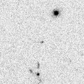
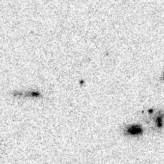
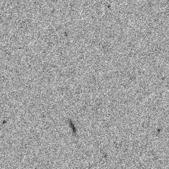
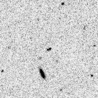
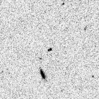
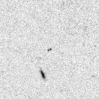
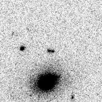
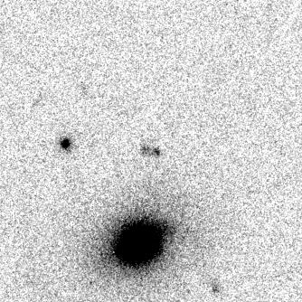
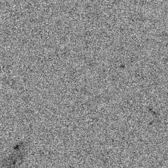
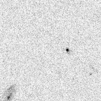
70 54 FIG stamps of each candidate in the narrowband, the four HST/ACS bands, and two Spitzer/IRAC bands. The circles are 2 in diameter, and are drawn to highlight the objects.

71 55 TABLE 3 CDF S LYα GALAXY CANDIDATES Name m AB (NB656) m AB (F606W) Rest EW (Å) Spectroscopic Conf. Object ± Object ± Object ± 5.9 z=3.19 Object ± 36.4 No Spectra Object ± 13.0 No Spectra Object ± NOTES. Object 3 is a known AGN at z = 3.19, and the line we detected in the narrowband filter is [Civ], thus the EW for object 3 is the [Civ] rest-frame EW for an object at z = The calculated rest-frame EWs for the other objects assume a redshift equal to that of Lyα at the center of the Hα filter, which is Objects 1, 2, 3 and 6 had grism spectra from the PEARS survey, thus we were able to spectroscopically confirm objects 1, 2 and 6 to be at z 4.4.

72 TABLE 4 MAGNITUDES OF CDF S LYα GALAXY CANDIDATES Name IAU Format Name m NB656 m B m V m i m z m Ch1 m Ch2 Obj 1 J Obj 2 J Obj 4 J Obj 5 J Obj 6 J NOTES. 3σ upper limits. Coordinates and magnitudes for each of our candidate Lyα galaxies. Each magnitude has been corrected to represent the total magnitude for the object. 56

73 57 and we found in the literature that it is a known [Civ] λ1549 emitter at z = 3.19 (Szokoly et al. 2004; Xu et al. 2007). This object was not included in our analysis Broadband Photometry For our analysis, we used the updated version of the GOODS CDF S catalog (ver. 1.9; M. Giavalisco et al in preparation) which has deeper observations in i and z, resulting in lower error bars for those two bands. As an external check on the photometry errors in the GOODS catalog, we used the Hubble Ultra Deep Field (HUDF; Beckwith et al. 2006) catalog. The HUDF is much deeper than the version 1.9 data in the same regions, thus any errors would be dominated by the v1.9 data. We matched the HUDF and v1.9 catalogs, then plotted the magnitude difference between the two versus the version 1.9 data for each of the four bands (B, V, i and z ). We characterized this error as being 1σ of the spread in the magnitude difference in a certain magnitude slice. This error was small ( < 0.1 mag in our magnitude regime), but in the cases where it was larger than the version 1.9 photometry error 7, we used this error in its place. When comparing data from different telescopes to models, we needed to be sure that the magnitudes we were using from our narrowband, ACS and IRAC data were defined the same way. In the narrowband, we obtained fluxes from PSF fitting, so then the magnitudes from these fluxes were total magnitudes. For the GOODS ACS data, we used the MAG AUTO magnitudes, which are known to be 5% fainter 7 The 1σ spread in the v1.9 photometry errors was 0.020, and mag for the V, i and z bands, respectively, at 26th magnitude.

74 58 than the total magnitude (Bertin 2006). Thus, we corrected the GOODS ACS data, adding on a factor of 5% to the flux to make them total magnitudes. The GOODS Spitzer IRAC data do not yet have a public catalog, but a catalog has been created using the TFIT software package (Laidler et al. 2007). TFIT uses a priori knowledge of spatial positions and morphologies from a higher resolution image (in this case the GOODS ACS z image) to construct object templates and fit them to the lower resolution image. However, this used the ACS catalog s MAG ISO parameter as a guideline for the radius of the galaxy, so in order to find the total magnitude, we added to the IRAC magnitudes the difference between MAG ISO and MAG AUTO for our objects in the ACS z catalog. We then added an additional factor of 5% to correct the IRAC magnitudes to be total magnitudes. We now had total magnitudes for our objects in nine bands, from B to 8.0 µm Modeling Stellar Population Models We have derived the physical properties of our candidate Lyα galaxies by comparing them to stellar population models, using the modeling software of Bruzual & Charlot (2003; hereafter BC03). Comparing to models allows one to choose a variety of physical parameters to see which matches the observations the best. We attempted to fit the following parameters for each galaxy: age, metallicity, SFH, mass and dust content. We used a grid of 24 ages ranging from 1 Myr to 1.35 Gyr (the age of the Universe at z = 4.4). We fit the objects to the full range of metallicity available with BC03, from to 2.5 Z. We modeled exponentially

75 59 decaying SFHs with characteristic decay times (τ) of 10 6, 10 7 and 10 8 yr. We also approximated an instantaneous burst/simple stellar population (SSP) by using an exponentially decaying SFH with τ = 10 3 yr, and a constant SFH with τ = yr. We included dust via the Calzetti dust extinction law (Calzetti et al. 1994), which is applicable to starburst galaxies, using the range 0 A Galactic dust was included from the method of Schlegel et al. (1998) with a value of E(B - V) = mag. We include intergalactic medium (IGM) absorption via the prescription of Madau (1995). The BC03 models do not tabulate any emission lines, but in order to model the dusty scenario we needed to include the Lyα emission line. We derived the Lyα line flux from the number of ionizing photons output for each model, assuming case B recombination (see Finkelstein et al. 2007; Chapter 2 for details). Some of our objects showed a stronger 3.6 µm flux than would have otherwise been expected. At z = 4.4, the Hα emission line would fall in this filter, so we also included an Hα emission line in the models (assuming case B recombination, the Hα line strength is times the Lyα line strength; Kennicutt 1983). In order to model the clumpy dust scenario, we needed to ensure that the Lyα line did not suffer dust attenuation. To do this, the continuum flux (and Hα flux) was multiplied by the Calzetti dust law before we added in the Lyα flux to the spectrum at the correct wavelength bin. In this case, the continuum suffers dust attenuation while the Lyα line does not. Lyα sits right at a step function in the Madau IGM treatment, so the amount of attenuation applied to Lyα depends strongly on the exact wavelength

76 60 position of the Lyα line. The accepted interpretation is that the internal kinematics of a given galaxy will result in half of the Lyα flux coming out slightly blue of the rest wavelength, and half slightly red. This results in the characteristic asymmetric profile of the Lyα observed in many spectra, where the blue side is truncated. We approximate this interpretation by attenuating the Lyα line to be approximately one half of its original (post-dust where applicable) flux. In order to go from the BC03 output flux to bandpass-averaged fluxes, we used the method outlined by Papovich et al. (2001). In short, we took the output from BC03, and converted it from L λ into L ν, and then from L ν into F ν (units of erg s 1 cm 2 Hz 1 ) using F ν = (1 + z) L ν / (4πd 2 L) to do the conversion and redshift the spectrum. This flux was then multiplied by the transmission function for a given bandpass (including the filter transmission and the quantum efficiency of the detector), and integrated over all frequencies. The bandpass averaged flux f ν is this result normalized to the integral of the transmission function. AB magnitudes (Oke & Gunn 1983) for the models were then computed Dust Effects on the Lyα EW The scenario we are probing observationally is whether or not dust could enhance the Lyα EW. Traditionally, it has been thought that Lyα galaxies could possibly be too primitive to have formed dust yet. However, some evidence does exist that would enable a galaxy to form dust quickly. Massive stars evolve on a very short timescale, so after a few Myr, a galaxy could begin to have some heavier elements in its ISM. Also, supersolar metallicities and CO emission have been seen in quasars at

77 61 z 6 (Pentericci et al. 2002; Bertoldi et al. 2003), and Lyα emission has been seen in submillimeter-selected galaxies (Chapman et al. 2004). However, even if Lyα galaxies did have dust, it has been thought that it would vastly attenuate the Lyα flux (Meier & Terlevich 1981). Lyα photons have long scattering path-lengths, making them extremely vulnerable to dust attenuation, assuming a uniform distribution of dust. It is possible that dust could be geometrically distributed such that the Lyα photons are attenuated less than the continuum. The most likely of these scenarios involves an ISM with clumpy dust clouds thoroughly mixed with neutral hydrogen within an inter-cloud medium which is tenuous and ionized (Neufeld 1991; Hansen & Oh 2006). Evidence for the possible existence of this scenario also comes from Giavalisco et al. (1996), who find a lack of correlation between UV slope and Lyα EW, meaning that a UV slope indicative of dust does not necessarily mean a low Lyα EW. They conclude that the ISM in their sample of galaxies is highly inhomogeneous, and that the transport of Lyα photons is primarily governed by the geometry of the ISM rather than the amount of dust. This is intriguing, because if Lyα galaxies had a dusty, inhomogeneous ISM then it is possible that the continuum photons were attenuated and the Lyα photons were not. Then the observed EW would be greater than the EW intrinsic to the underlying stellar population by a factor relating to the amount of dust present. To better understand this, we will follow the journey of a photon through an ISM, starting from the point when it is emitted from a massive star. This star will emit numerous ionizing photons, 2/3 of which will become Lyα photons assuming case B

78 62 recombination. When a Lyα photon encounters a region of dust mixed with neutral hydrogen, it has a very high probability of being absorbed by the first hydrogen atom it encounters. It will then be reemitted in a random direction, with an equal chance of being sent back the way it came as being sent forward in its original direction of travel. If the ISM is uniformly distributed, the Lyα photon will only move a short distance before it is absorbed again, requiring a very long time for a given Lyα photon to escape the galaxy. If the ISM is composed of clouds in a nearly empty inter-cloud medium, then when a Lyα photon is emitted back out of the clump, 8 it will travel a long distance before it encounters another clump, vastly increasing the probability that it will escape the galaxy. Even if it is re-emitted in the direction further into the clump, it will still be scattered close to the surface, so it still has a chance to escape. However, continuum photons in a homogeneously distributed ISM will be absorbed by dust as they travel through the ISM. Since their wavelengths are continuously distributed, they will essentially be unaffected by the presence of neutral hydrogen. The same holds true in a clumpy ISM. A continuum photon will be able to bypass the hydrogen in the clump until it encounters a dust grain, at which point it could either get scattered or absorbed. If the continuum photon is absorbed, it will eventually be reemitted, but its wavelength will have changed to the far-ir. The net effect of this is to lower the amount of continuum flux escaping the galaxy (as well as to redden the flux due to those photons which are scattered rather then absorbed). 8 The probability of a Lyα photon being absorbed in a clump is 2 ǫ, where ǫ is the single scattering albedo (Hansen & Oh 2006). This is valid for ǫ 1, where ǫ = 0 signifies complete reflectance)

79 63 Thus, a clumpy ISM could result in a higher Lyα EW than the underlying stellar population. It has been generally believed that Lyα galaxies are very young, primitive objects. If we find proof that an object shows dust enhancement of the Lyα EW, it could turn out that some fraction of Lyα galaxies known to exist could in fact be older, more evolved stellar populations, changing our view of where Lyα galaxies belong in the galaxian zoo IGM Inhomogeneities Although differences in the IGM can affect the models in the V band, we chose to include this band in our fits. The V -band is complicated, as at z = 4.4 it contains the entire Lyα forest region from the Lyman limit out to Lyα. To account for inhomogeneities in the IGM, we chose to include a flux variance for the model V -band flux (this results in a second parameter in the denominator for the V -band χ 2 term; see 3.5.1). To account for IGM absorption in our models, we have attenuated the cumulative flux which comes out of BC03 by a factor of exp(-τ IGM ), such that the bandpass averaged flux in the V -band is given by f V = λ2 λ 1 f BC03,λ e (τ λ+δτ λ ) dλ (4) where f BC03,λ is the initial output of the models and δτ λ is the 1σ error in the IGM optical depth due to inhomogeneities among different lines of sight. We can then break this up into a sum over discrete intervals, and calculate the variance, which for a small δτ λ is N σ f 2 V = ( ) fbc03,λ 2 e τ λ 2 (δτ λ ) 2 λ 2 (5) n=1

80 64 where N is the number of bins we chose to break the V -band into. We approximate this as σ 2 f V = N (δτ λ ) 2 F 2 V N 2 ( e τ λ ) 2 (6) where F V 2 is the total flux in the bandpass. The rms flux in the V -band due to the IGM inhomogeneities is then σ = F BC03,V e τ δτn 1 2 (7) Thus the fractional error in the model flux which needs to be added in is δτ N 1 2. To make this physically correct, the bin size should be equal to a typical clustering length for Lyα forest clouds, such that the Lyα forest optical depth variations in adjacent bins are essentially uncorrelated. Penton et al. (2000) calculated the twopoint correlation function for Lyα forest clouds. They found that the correlation drops to zero at a separation of 11 Mpc. For z = 4.4, the co-moving distance between the front and back of the V -band filter is 1205 Mpc. Thus, we chose to use 110 bins. The uncertainty in the IGM absorption (δτ) was found from Madau (1995). Extrapolating from his example of a z 3.5 galaxy, we found an uncertainty in exp(-τ) of 0.35, which corresponds to δτ = Plugging these values into the above equations, we find that we need to include an error of 0.1 mag for the V -band model fluxes to account for inhomogeneities in the IGM Equivalent Widths Model Lyα equivalent widths were calculated using the ratio of the model flux in the Lyα wavelength bin to the average continuum value on either side of that bin ( λ). We compare our model EW distribution to previous studies (i.e. Charlot & Fall

81 ; Malhotra & Rhoads 2002; hereafter MR02). We also quantify the multiplicative effect adding clumpy dust to the models has on the Lyα EW. Figure 7 shows the EWs of our models plotted versus stellar population age for Z=.02Z and three different star formation histories: SSP (single burst), τ = 10 7 (exponentially decaying) and a constant star formation history. We first discuss the results from the left-hand vertical axis, which shows the EWs from dust-free models. All of the models start at some value ( 400 Å) at 10 6 yr and then decay from there. The EWs from the SSP and τ models fall all the way to zero at approximately 30 and 100 Myr, respectively. Models which are constantly forming stars asymptotically reach a constant value of EW at 120 Å due to the constant replenishment of massive stars. The upturn at later ages for the SSP and τ models are due to either hot horizontal branch stars and/or planetary nebula nuclei, which will start to dominate the UV flux after 10 8 yr. While technically their Lyα EWs will be high, the actual UV continuum flux is tiny compared to what it was at earlier ages, and thus objects in this stage will likely not appear in Lyα galaxy samples. We calculate that at 400 Myr (the age at which the UV-upturn causes the EW to surpass 50 Å) a mass in excess of M would be required in order for a given stellar population to be detected in our narrowband image. This mass is extremely high even in local universe terms (e.g., Tremonti et al. 2004), and thus is not likely to exist at high redshift. In order to distinguish EWs due to young stars from EWs due to faint UV continuum flux, the solid lines in these plots change to dashed lines when the continuum (V -band) flux falls to 10% of its value at 10 6 yr.

82 66 Charlot & Fall (1993) computed the Lyα EW from stellar population models using an earlier version of the Bruzual & Charlot software (1993). Their models assumed solar metallicity and case B recombination. They computed the Lyα EW for multiple IMF slopes, upper-mass cut-offs and star formation histories, with their youngest age being 5 Myr. For a SSP with a near-salpeter IMF (x = 1.5; x Salpeter = 1.35) their maximum EW was calculated to be 210 (240) Å for an upper-mass cut-off of 80 (120) M, falling to zero at 40 Myr. The EWs from our SSP model have a maximum value of 400 Å (only 100 Å at t = 5 Myr), falling to zero by Myr. However, their definition of SSP differs from ours. We defined ours as having a characteristic decay rate of 10 3 yr, while their burst model had a timescale of 10 7 yr. We can thus compare their results to our τ model (which has τ = 10 7 yr). This model has a maximum EW of 400 Å ( 200 Å at 5 Myr), much closer to the results of Charlot & Fall. For a constant SFH, Charlot & Fall find a maximum Lyα EW of 150 (250) Å falling to a constant value of 90 (100) Å by 10 8 yr for an upper-mass cut-off of 80 (120) M (our upper-mass cut-off was 100 M ). Our continuously star-forming models start at a maximum EW of 400 Å ( 220 Å at 5 Myr), falling to 120 Å by 10 8 yr. Taking into account the differences between IMF slopes, metallicities and upper-mass cut-offs, we feel our constant SFH models are consistent with those of Charlot & Fall. In a more recent study, MR02 did a similar analysis using Starburst99 models (Leitherer et al. 1999). Their Salpeter IMF model has a constant SFH, upper-mass cut-off of 120 M and Z = 0.05 Z. The EW from

83 FIG. 7. Equivalent width distribution from the models for Z =.02 Z. The upturn in EW at late age is caused by either hot horizontal branch stars and/or planetary nebulae nuclei, either of which will dominate the UV flux at later ages. However, at this point the total UV flux is much less that it was at early ages, such that a stellar population this old would likely not be picked up in a narrowband selected survey. Due to this, the line-style changes to dashed at the point where the V-band flux drops below 10% of its value at 10 6 years. The left-hand axis shows the rest-frame EW with no dust, and the right-hand axis shows the rest-frame EW with A 1200 = 2.0. In order to observe a galaxy with an EW > 200 Å, it either needs to be only a few Myr old with no dust, or with dust it can be older than 10 Myr. Comparison to previous studies (Charlot & Fall 1993; Malhotra and Rhoads 2002) shows that our model EWs are consistent with previous results. 67

84 68 this model had a maximum value of 300 Å at an age of 1 Myr, asymptoting to a value of 100 Å by 100 Myr, both of which are consistent with our models. When clumpy dust comes into the models, things can change dramatically. As we discussed above, in our models the dust is not attenuating the Lyα line, which results in the Lyα EW being enhanced as the continuum is suppressed. Consequently, given an amount of dust extinction, the Lyα EW will be enhanced by a multiplicative factor. For dust amounts of A 1200 = 0.5, 1.0, 1.5 and 2.0 mag, this factor is 1.64, 2.68, 4.40 and 7.21, respectively. The right-hand vertical axis in Figure 7 shows what the EWs from the models are with 2.0 mag of clumpy dust extinction. This shows that for a given model, one can have an older age while still keeping a high EW. For example, for a SSP with Z = 0.02 Z, the EW drops below 200 Å by 3 Myr, while with 2.0 mag of clumpy dust, this does not happen until after 10 Myr, over a factor of three times longer, making it much more likely that this object would be observed with a high EW in a narrowband selected survey. Table 5 shows the maximum possible age allowed for a stellar population with EW < 200 Å for a variety of models Results Fitting to Models Using our bandpass averaged fluxes, we were able to fit our objects to the BC03 models. We have nine possible bands to choose from for fitting: CTIO-MOSAIC Hα, HST/ACS F435W (B), F606W (V ), F775W (i ), F850LP (z ), Spitzer/IRAC channel 1 (3.6 µm), channel 2 (4.5 µm), channel 3 (5.8 µm) and channel 4 (8.0 µm). In order to separate the model-dependent parameters from other factors, we elected to fit flux

85 69 ratios to the models, and then fit the mass to the best-fit model at the end. We computed a flux ratio to the i band for each band, with a corresponding flux ratio error propagated through. The χ 2 was then computed for each model object combination using: [ f i obj fmod i (t, τ, A 1200, Z) ] 2 χ 2 = i σ 2 (f i obj ) (8) where i denotes the bandpass, f obj is the object flux ratio, f mod is the model flux ratio and σ(f obj ) is the error in the flux ratio for a given bandpass, derived from the error in the flux for each bandpass and the error in the i -band flux. All fluxes were in units of f ν (ergs s 1 cm 2 Hz 1 ). Out of our five Lyα galaxy candidates, we only fit stellar population models to four of them. While we have no reason to suspect object 5 is not a real Lyα emitter, its proximity to a very bright object makes its Spitzer fluxes inaccurate. With only the ACS and narrowband data to go on, there are not enough available passbands to fit this object. Thus the four objects which we fit were: 1, 2, 4 and 6. While we did have data in all nine bands listed above, not all were used in our fitting. Both the IRAC 5.8 and 8.0 µm were undetected in the four objects we fit, and thus were not used. Because the entire B-band is blue-ward of the Lyman break, we can be highly confident that on any line of sight there will be no significant flux transmitted through the B-band. If redshift were a free parameter in our models, then we would definitely use the B-band, as the absence of flux would be a helpful redshift indicator. However, given that three of our four objects were spectroscopically confirmed (and the fourth has a photo-z) to be at z = 4.4, we did not feel it would be worthwhile

86 TABLE 5 MAXIMUM POSSIBLE AGE ALLOWED FOR A STELLAR POPULATION WITH EW > 200 Å SFH No Dust A 1200 = 2.0 Z =.02*Z Z = Z Z =.02*Z Z = Z SSP 3 Myr (182 Å) 1 Myr (193 Å) Myr ( Å) 5 6 Myr ( Å) τ = Myr (184 Å) 3 Myr (186 Å) Myr ( Å) Myr ( Å) Constant SFH 8 Myr (193 Å) 3 Myr (190 Å) Never Never NOTES. Values in parenthesis are the Lyα equivalent widths at the reported ages. Since the grid of model ages is not continuous, in some cases there is a large amount of time around when the EW drops below 200 Å in the models. In these cases we report the ages and EWs on either side of 200 Å. Depending on the star formation history and metallicity, two magnitudes of clumpy dust extinction can keep the Lyα EW above 200 Å up to 3 20 times longer than just young stars alone (indefintiely for a population which suffers no drop in star formation activity). Models with dust have q = 0 (see 3.5.1). 70

87 71 to introduce redshift as a free parameter. Thus we have left the B-band out of the fitting. As a final step, we introduced a parameter, q, which we called the clumpiness parameter because its value simulates the effects of different dust geometries. Previously, when we applied dust to the models, we added in the Lyα flux after the dust was added, so that the Lyα flux was not attenuated. This had a very cartoon effect on the models, meaning that Lyα was either attenuated by all of the dust or by none of the dust. We still proceed in the same order as before, only now we multiplied the Lyα flux by e qτ, with q ranging from 0 to 10. A q value of zero represents exactly what our original models had been doing, by not attenuating Lyα by dust. This models the dust geometry of clumpy clouds in an empty inter-cloud medium, i.e., Neufeld (1991) and Hansen & Oh (2006). A q value of 10 attenuates Lyα 10 times more than the continuum. Thus, q 10 models the effects of a uniform dust distribution, attenuating Lyα much more than the continuum due to the fact that it is resonantly scattered. Values between 0 and 10 model differing geometries, with the case of q = 1 modeling a geometry where Lyα and the continuum are attenuated at the same rate (possibly a scenario with dust in clouds, but in which the inter-cloud medium is not entirely empty). Introducing this parameter vastly increased the quality of the best fits, but it did come at a cost. Since we had no additional data, we could not add another free parameter without taking away one. We decided to remove metallicity as a free parameter, as the effects of changing metallicity had the least effect on the models. We decided to fix a value of Z =.02 Z for all models.

88 Object 1 Object 1 is best fit by a 5 Myr stellar population with a mass of M, a continuous star formation history, and 1.1 mag of dust extinction (A 1200 ) which attenuates Lyα 50% more than the continuum (q = 1.5). The quality of this fit was high, with χ 2 r = This object is thus very young, but its red color (specifically, z µm) indicates a significant amount of dust. However, an object this young, especially with a continuous SFH, already has a pretty high Lyα EW. Thus, even though it is best fit by a significant amount of dust, it does not require this dust to enhance its EW, as evidenced by its value of q > 1. This object fits the mold of a typical Lyα galaxy, as it is young and low mass. This being said, its dust content is intriguing as it indicates that this object is definitely not primitive Object 2 Object 2 is also best fit by a young, low-mass stellar population (3 Myr; M ), however it has a fast-decaying SFH, with τ = 10 6 yr. It has less dust than object 1 (A 1200 = 0.9 mag), but a larger value of q, with q = 2 indicating that Lyα is being extinguished at twice the value of the continuum. However, we should be somewhat skeptical about these results, as this object has the worst fit out of our sample, with χ 2 r = That being said, these results are not astonishing, as they indicate that this object is possibly very similar to object Object 4 Object 4 is the most intriguing object in our sample. It has the highest quality fit of the whole sample, with χ 2 r = 1.326, lending the most credibility to its results.

89 73 It is best fit by an 800 Myr, M stellar population with a continuous SFH. While the amount of dust extinction is lower than the other objects (A 1200 = 0.4 mag) it has a value of q = 0, the only object with q < 1.5. While 0.4 mag of dust is not a lot, if it is not attenuating Lyα, as q = 0 attests to, it will increase the EW by 50%, making this object a candidate for dust enhancement of the Lyα EW. This object definitely does not fit the mold of a typical Lyα galaxy with its old age and larger mass. Although we only have one object like this in our small sample, its existence means that Lyα galaxies may not all be uniformly young Object 6 Similar to objects 1 and 2, object 6 is also best fit by a young (3 Myr) and low-mass ( ) stellar population. It has an exponentially decaying SFH with τ = 10 6 yr and 1.8 mag of dust attenuating Lyα 50% more than the continuum. The best-fit model (χ 2 r = 2.121) has a low EW of 61 Å, which is very comparable to the measured EW of the object, which was 56 Å. Although this object has a young age, its fast-decaying SFH and large amount of dust which is attenuating Lyα are keeping the Lyα EW down. Figure 8 shows the best-fit models for each object, and Table 6 details the best-fit parameters Best-Fit Models Without Dust As an exercise, we wanted to see what the best-fit models to these objects would be if we forced the amount of dust to be zero while keeping everything else the same. In doing this, the number of degrees of freedom became three, because both dust and q were dropped as free parameters, thus the reduced χ 2 reported is

90 74 χ 2 /3. Figure 9 shows the results of this analysis. With no dust, all of the objects were forced to have an older age to explain the red colors. In all cases, the best-fit model with no dust had a significantly higher χ 2 r than the best-fit model allowing dust, thus we can be reasonably sure that these objects have some dust, and that we have treated it correctly in the models Monte Carlo Analysis To determine confidence regions for our model parameters, we ran 10 4 Monte Carlo simulations. In each simulation, we add or subtract flux to each band for each object equal to a Gaussian random deviate multiplied by the object s flux error in a given band. Each band had its own random number in each simulation, which was computed by the IDL function RANDOMN, which generates Gaussian distributed random numbers. For each possible model (25200 possible models; 5 SFHs, 24 ages, 21 dust optical depths and 10 values of q), the χ 2 was computed for each simulated object flux. The result was that for each object, we now had 10,000 best-fit models. In an ideal case, these models would be distributed around the best-fit parameters to the actual observations. In order to see if this was true, we plotted contours showing the density of best-fit parameters for each object in three planes: dust versus age, dust versus q and age versus q (Figure 10). 9 The blue, green and red contours show the 1 σ (68%), 2 σ (95%) and 3 σ (99.5%) confidence levels, respectively. For object 1, it appears as if 9 We acknowledge that we are prevented from observing part of the dust vs. q plane due to selection effects. A galaxy with A 1200 = 2.0 and q = 10 would have its Lyα much too supressed to be selected via the narrowband. Similarly, a galaxy with A 1200 = 2.0 and q = 0 would be bright in the narrowband, but its continuum flux would be vastly attenuated, thus an object such as this may not have enough data to be used in a stellar population study.

91 FIG. 8. The open circles are centered on the positions of the bandpass averaged fluxes of the best-fit models. Object 1 is best fit with a young, low-mass stellar population with a continuous SFH. The best-fit model contains over a magnitude of dust, but its geometry is such that it is extinguishing Lyα 50% more than the continuum. Object 2 is best fit by a young, low-mass stellar population with an exponentially decaying SFH with τ = 10 6 yr. There is a little less than a magnitude of dust, but it is extinguishing Lyα at twice the amount of the continuum. Object 4 is by far the most interesting object in our sample. It is best fit by a much older, higher-mass stellar population with a continuous SFH. It has less dust that the other models, but this dust is not attenuating Lyα at all, enhancing the observed Lyα EW. The combination of dust and a continuous SFH is allowing this object to have a high EW at an age of 800 Myr. Object 6 is best fit by a young, low-mass model similar to objects 1 and 2. However, the best-fit model has nearly 2 mag of dust attenuating Lyα twice as much as the continuum, resulting in a lower EW. 75

92 76 TABLE 6 CDF S BEST-FIT PHYSICAL PARAMETERS Name χ 2 r Age Mass A 1200 SFH q (Myr) (M ) (mag) Object Continuous 1.50 Object τ = Object Continuous 0.00 Object τ = NOTES. The best-fit parameters for each of our objects. These were found by minimizing the reduced χ 2 between each object and a grid of models.

93 FIG. 9. Best-fit stellar populations forcing the models to have no dust. All objects are best fit by older, more massive stellar populations, but the quality of these fits are of much lower quality (higher χ 2 ) than the best-fit models with dust. 77

94 78 the age is well constrained to be very young, as the 1 σ contour is fairly thin along the age axis. The same is true for q, constraining it to be between 1 and 3, ruling out dust enhancement of the Lyα EW for this object. The only parameter that may be degenerate is dust, as the 1 σ contour is very long along the dust axis. However, in no case is any model best fit with zero dust, and the 1 σ contour is roughly centered on the best-fit value of A 1200 = 1.1. Object 2 is very similar to object 1 in that its age is well constrained to be young, and its q value is well constrained to be greater than 1. Similarly, the dust in object 2 is slightly degenerate, but it is well constrained to have some dust, with the best-fit value being the most likely value. The age of object 6 is also well constrained to be young, although there is a slight 1 σ blip at t = 100 Myr. The q value is even better constrained than in objects 1 or 2, being very centered on the best-fit value of 1.5. Dust is still degenerate, although less so than in objects 1 or 2, with 1 σ values ranging from 1.5 to 2.0 mag. Object 4 is the only object in our sample which shows evidence of dust enhancement of the Lyα EW. The age is mostly constrained to be > 100 Myr, with a large 1 σ area centered around the best-fit model at 800 Myr, and a smaller 1 σ area around 200 Myr (and an even smaller one at 30 Myr). A range of dust values are permitted, but generally lie in the range from 0.1 to 0.9 mag. The q parameter is definitely constrained to be < 1, with the 1 σ area centered around the best fit, with no part of it being greater than q = Thus this object is well constrained to have an old age and a small amount of dust with a dust geometry which is enhanc-

95 79 ing the Lyα EW. It should be noted that the effect of dust is not enormous. Dust extinction of 0.4 mag will increase the Lyα EW by 50%, meaning that the EW of this object was not negligible beforehand, mainly due to a constant SFH. However, the dust pushes this object s best-fit model EW from a value of 120 up to 180 Å. Given the model EW curves we saw earlier, if one ignored the possible effects of dust one would expect to see many more 120 Å EW objects than 180 Å. While this effect is only seen in one object, it shows that we cannot afford to ignore the effect dust could have on Lyα EWs, as we have shown it can help explain the perceived over-abundance of high-ew sources Discussion Lyα Detection Fraction Out of the whole GOODS CDF S catalog, we found that there were 229 B- band dropouts. The dropout criteria selects galaxies with a z range of 1.0. The width of our narrowband filter is 80 Å around a central wavelength of 6563 Å, corresponding to a z range of 0.07 for Lyα. Thus, about = 16 B-dropouts lie in the redshift range where we could detect Lyα. Among these, only five show a narrowband excess. This corresponds to a Lyα detection fraction of 31%, comparable with previous studies (e.g., Shapley et al. 2003; 25%) Hα Equivalent Widths When comparing the best-fit models to the data points, it is obvious that the model Hα flux is dominating the model 3.6 µm flux, as is evident from the fact that the 3.6 µm data point is far above the model continuum level. The model rest-frame

96 (a) FIG. 10. (a) Contours showing the density of results from our Monte Carlo simulations. Each asterisk represents the best fit of one Monte Carlo run (most of the asterisks are really multiple points). The rest of the model grid which did not have a best fit are denoted by dots. The best-fit model from the actual object is denoted by a blue triangle. The objects are in separate rows, and the columns represent three different planes: dust vs. age, dust vs. q and age vs. q (note that the range of the age axis is different for some of the objects). Continued on next page... 80

97 (b) FIG. 10. (b) Sixty-eight percent of the best fits from the simulations fall in the blue contour, and as such this is the 1 σ contour. Likewise, the green is the 2 σ contour and the red is the 3σ contour. The cross-hatched region represents the area of parameter space where we would not expect to detect an object due to dust extinction. Models falling in this region had their V or NB656 band flux reduced to less than a third of that of the best-fit model. Studying these figures, we were satisfied that our best-fit models accurately represented the most-likely best fit for each object. 81

98 82 Hα EWs are 3800, 8500, 200 and 1700 Å for objects 1, 2, 4 and 6, respectively. At first glance, these seem large, but one needs to remember that with the exception of object 4, these objects have been found to be extremely young, low-mass, star-forming galaxies. Keeping that in mind, these values of Hα EW are quite reasonable. In a survey of Hii regions in a nearby galaxy, Cedres et al. (2005) found that the Hα EW distribution peaked at 1000 Å, with a few Hii regions with EWs as high as Å. In an analysis of a z = 6.56 Lyα galaxy, Chary et al. (2005) derived an Hα EW of 2000 Å, concluding that the Hα line dominated the 4.5 µm flux in their object. While computing the synthetic properties of starburst galaxies, Leitherer and Heckman (1995) computed a Hα EW of 3200 Å for a population with 0.1 Z and a constant star formation history. Taking into account model differences (including a difference of 5 times in metallicity) we find our values of Hα EWs to be consistent with those previously found in the literature for star-forming galaxies. The addition of Hα flux to the model spectra led to an interesting result. In a young star-forming galaxy both Lyα and Hα photons will be produced in large quantities, producing the large Lyα and Hα EWs seen in objects 1, 2 and 6. However, if the Lyα EW is only observed as being large due to dust enhancement, than the Hα EW should not be large (as Hα photons are not resonantly scattered). This is seen in our sample, as object 4 has a best-fit Hα EW of only 200 Å, much less than the other three objects. Thus, obtaining data about Hα lines in Lyα galaxies could be an important diagnostic for deciphering the underlying stellar population, as the Lyα/ Hα ratios should indicate whether dust enhancement is playing a role. This

99 83 tool will be a prime candidate for study on future observatories such as the James Webb Space Telescope or the Stratospheric Observatory for Infrared Astronomy Comparison to Other Work It is useful to compare our results to those of other studies done using HST and Spitzer data together, as the IR data (which corresponds to the rest-frame optical at z = 4.4) better constrains the stellar masses as it is less attenuated by dust than the rest-frame UV. Two recent studies have been published studying Lyα emitting galaxies (LAEs) at z 5 and 5.7 by Pirzkal et al. (2007) and Lai et al. (2007), respectively. Pirzkal et al. studies the stellar populations of nine LAEs in the HUDF detected on the basis of their Lyα emission lines in the Grism ACS Program for Extragalactic Science (GRAPES; Pirzkal et al. 2004; Xu et al. 2007; Rhoads et al. 2008) survey. Using stellar population models similar to ours, they found very young ages ( 10 6 yr) and low masses ( few 10 7 M ), with some dust in a good fraction of their objects. Lai et al. studied three narrowband-selected LAEs spectroscopically confirmed to lie at z 5.7 in the GOODS HDF-N field. Also using BC03 models, with an instantaneous burst SFH they found ages from 5 to 100 Myr (up to 700 Myr with a constant SFH), and masses from 10 9 to M. Their objects were also best fit by dust, with E(B - V) (A V 1 1.2). Three of our four objects have ages consistent with those from Pirzkal et al. (2004) and Lai et al. (2007), who find ages from 1 to 100 Myr. Our fourth object has an age much larger than those found in these papers, at 800 Myr. Eight out of the nine Pirzkal et al. objects have M < 10 8 M, whereas the Lai et al. objects

100 84 have masses 2 orders of magnitude higher. The masses of our objects reside in the middle, from 10 8 to 10 9 M. The likely reason that our masses are higher than those of Pirzkal et al. is because they reach fainter luminosities, detecting objects with emission lines as faint as erg s 1 cm 2. On the flipside, the larger masses from Lai et al. are likely due to their selection criteria. They found 12 LAEs in the GOODS-N field, but they only analyzed the three objects with significant 3.6 and 4.5 µm flux. They acknowledge that their masses are high, and that this may be due to selecting objects from the high-mass end of the mass distribution. Another difference is how each study treated Lyα in their model fitting. Pirzkal et al. chose to exclude the ACS i band from their fitting, as at their redshifts the Lyα line would fall in this band, and they did not want to include the uncertainties that subtracting the line flux from the i flux would create. Lai et al. chose to treat Lyα by estimating the amount of flux Lyα contributed to the i flux, then adding this percentage as an i -band error ( 30%). As described in detail in earlier sections, we chose to add the Lyα emission to the models in order to investigate the effect dust had on the Lyα EW. While each of these methods has its merit, the method of Pirzkal et al. likely introduces the least amount of uncertainty by simply not including the broadband which contains the Lyα emission. They had the luxury that in addition to the ACS and IRAC data, they also had HST NICMOS and Very Large Telescope (VLT) ISAAC near-ir data, so cutting a band from the fitting did not force them to throw out a constraint.

101 85 One other interesting study is that done by Chary et al. (2005) by fitting stellar population models to a z = 6.56 Lyα galaxy with near-ir and IRAC data. As we mentioned above, they determined that their 4.5 µm flux was dominated by a Hα line, implying vigorous star formation. Taking this line into account, they found a best-fit stellar population of 5 Myr, M with A V = 1.0 mag. This is even dustier than our objects, showing that not only is dust common at z = 4.4, it may exist in Lyα galaxies up to z 6.5. By including Lyα in our models rather then attempting to subtract out its influence in the observed broadbands, we were able to investigate the effect dust geometry had on the Lyα EW. While the other two studies listed here did not do this analysis, they did include homogeneous dust in their models. They found that many/all of their objects were best fit by including at least a small amount of dust. This confirms our result that regardless of the effect of the dust geometry, one needs to include dust when analyzing LAEs, as it appears to be present in a majority of them. Failure to include dust in the models will result in a poorer fit, likely with an older or more massive stellar population than is really in place Conclusions We have presented the results of our analysis of four narrowband selected Lyα galaxies in the GOODS CDF S. By observing in such a well studied field, we were able to take advantage of the plethora of deep public broadband data (GOODS HST ACS, Spitzer IRAC and MUSIC), as well as previous spectroscopic studies (PEARS)

102 86 available in the region. Three out of our four objects were spectroscopically confirmed to lie at z = 4.4. The other object has a photometric redshift of Previously, it had been assumed that Lyα galaxies were young, low-mass galaxies with little to no dust. Even when dust has been found, it has been assumed to be homogeneously distributed, meaning that it would attenuate the Lyα flux much more than the continuum flux because Lyα photons are resonantly scattered. However, a scenario has been theoretically studied in which the geometry of a dusty ISM could actually enhance the Lyα EW rather than reduce it. This scenario consists of an ISM in which the dust resides in clouds, mixed in with neutral hydrogen, whereas the inter-cloud medium is hot and ionized. In this scenario, Lyα photons would effectively bounce off the surface of the clouds, finding it much easier to escape the galaxy than continuum photons. Thus, a galaxy could exhibit a much larger Lyα EW than that intrinsic to the underlying stellar population. In order to investigate this, we have compared the fluxes of our objects to stellar population models. We have included Lyα emission in the models, as well as introducing a clumpiness parameter, q, which dictates how much Lyα is attenuated by a given dust amount. Three of our four objects were best fit by models with a very young age ( few Myr) and low stellar masses ( few 10 8 M ), with a significant amount of dust (A 1200 = ) attenuating the Lyα flux more than the continuum (q = ). However, one object, object 4, is best fit by a vastly different model. This object is best fit by a much older, more massive stellar population, with an age of 800 Myr and M = M. What is interesting about this object is that

103 87 its EW is among the highest in our sample. Even with a constant SFH, an 800 Myr stellar population would not be able to produce a Lyα EW above 120 Å, while this object has an observed rest-frame EW of 150 Å and a best-fit model EW of 180 Å. Thus something is causing the EW of this object to be enhanced, and the models tell us that it is due to dust. This object is best fit by A 1200 = 0.4 mag of dust, and while this is less than any of the other objects, the clumpiness parameter is best fit to be q = 0.0. This means that the 0.4 mag of dust are attenuating the continuum, but not the Lyα flux, enhancing the EW by 50%. Comparing our results to those from other studies, we find that our age and mass results are consistent when data and selection differences are accounted for. However, no other observational studies have yet tried to model the effect dust could have on Lyα for differing geometries. While our sample size is small, analysis of a larger sample could indicate that there are really two classes of Lyα galaxies: a young, low-mass Lyα galaxy with an intrinsically high Lyα EW and an older, higher-mass galaxy with a lower intrinsic EW which has been enhanced due to dust.

104 4. Lyα GALAXIES: PRIMITIVE OBJECTS, DUSTY STAR-FORMERS OR EVOLVED GALAXIES? 4.1. Abstract We present stellar population modeling results for 11 newly discovered Lyman alpha emitting galaxies (LAEs), as well as four previously known LAEs at z 4.5 in the Chandra Deep Field South. We fit stellar population models to these objects in order to learn specifically if there exists more than one class of LAE. Past observational and theoretical evidence has shown that while many LAEs appear to be young, they may be much older, with Lyα EWs enhanced due to resonant scattering of Lyα photons in a clumpy interstellar medium (ISM). Our results show a large range of stellar population age (3 500 Myr), stellar mass ( M ) and dust extinction (A 1200 = mag), broadly consistent with previous studies. With such a large number of individually analyzed objects, we have looked at the distribution of stellar population ages in LAEs for the first time, and we find a very interesting bimodality, in that our objects are either very young (< 15 Myr) or old (> 450 Myr). This bimodality may be caused by dust, and it could explain the Lyα duty cycle which has been proposed in the literature. We find that eight of the young objects have SEDs consistent with a clumpy ISM. We find that dust geometry appears to play a large role in shaping the SEDs that we observe, and that it may be a major factor in the observed Lyα equivalent width distribution in high redshift Lyα galaxies, although other factors (i.e. outflows) may be in play. We conclude that 13 out of our 15 LAEs are dusty star-formers, with the other two LAEs being evolved galaxies.

105 Introduction While high-redshift galaxies can be hard to observe due to dimming with distance, narrowband selection of Lyα galaxies has proven a very efficient method to select high-redshift galaxies based on a strong emission line (e.g., Rhoads et al. 2000, 2004; Rhoads & Malhotra 2001; Malhotra & Rhoads 2002; Cowie & Hu 1998; Hu et al. 1998, 2002, 2004; Kudritzki et al. 2000; Fynbo, Möller, & Thomsen 2001; Pentericci et al. 2000; Ouchi et al. 2001, 2003, 2004; Fujita et al. 2003; Shimasaku et al. 2003, 2006; Kodaira et al. 2003; Ajiki et al. 2004; Taniguchi et al. 2005; Venemans et al. 2002, 2004; Pascarelle et al. 1996ab; Gawiser et al. 2006a; Lai et al. 2007, 2008; Nilsson et al. 2007; Finkelstein et al. 2008a). These objects are of interest, as over 40 years ago Partridge & Peebles (1967) proposed that they may be signs of primitive galaxies in formation. This was easy to understand, as Lyα photons are copiously produced in star formation regions, and we would expect the first galaxies to be undergoing periods of extreme star formation. However, not until recently have we had the data to verify this assumption. The availability of stellar population modeling codes has allowed the derivation of physical parameters of galaxies from photometry alone. In the past few years (thanks to large surveys such as the Great Observatories Origins Deep Survey (GOODS)), broadband photometry of LAEs has become deep enough to compare objects to these models, learning about such parameters as stellar population age, stellar mass, and dust extinction. First results from these studies were unsurprising, as stacking analyses showed that an average LAE was young ( Myr), low

106 90 mass ( M ) and dust free (e.g., Gawiser et al. 2006a; Finkelstein et al. 2007, Chapter 2; Lai et al. 2008). Recently, deeper data has allowed the comparison of individual high-redshift LAEs to models for the first time, as chronicled in Chary et al. (2005), Pirzkal et al. (2007), Lai et al. (2007) and Finkelstein et al. (2008a, Chapter 3). These studies have shown a wide range of results, with LAE ages from Myr, masses from M and, most surprisingly, dust extinction with A V up to 1.3 mag. These results show that while some LAEs may be young and dust-free, many are dusty, and some are even evolved (i.e. old and high mass). This raises an interesting question, as how can an evolved stellar population produce enough Lyα photons to be picked up by a narrowband selected survey? Many scenarios have been proposed (i.e. zero metallicity, top-heavy initial mass function etc.), but these are rather extreme, and given the amount of dust extinction we see, they would be unlikely to produce enough Lyα photons to explain the observed excesses. We have thus decided to observationally test a scenario developed theoretically by Neufeld (1991) and Hansen & Oh (2006), where the Lyα equivalent width (EW) actually gets enhanced due to a dusty interstellar medium (ISM). This is counterintuitive, as dust will strongly suppress any ultraviolet (UV) photons. The news is even worse for Lyα photons, as they resonantly scatter off of neutral hydrogen atoms, thus their mean-free-paths are rather small, vastly increasing their chances of encountering a dust grain. However, as Neufeld and Hansen & Oh suggest, an ISM that is very clumpy could actually prevent the Lyα photons from seeing the dust at all. This can happen if the dust and neutral hydrogen lie in clumps, with a tenuous, ionized

107 91 medium separating the clumps. In this geometry, the Lyα photons stand a very high chance of being resonantly scattered at the surface of these clumps, spending most of their time in the inter-clump medium. In this manner, the Lyα photons are effectively screened from ever encountering a dust grain. The story is different for continuum photons, as they are not resonantly scattered, thus they will penetrate deeply into a clump, with a strong chance of being scattered or absorbed. As EW is a measure of line-to-continuum flux, this effectively enhances the observed EW over that due to the stars (or more accurately, the stars interaction with the interstellar hydrogen in their immediate surroundings). Note that the Lyα flux itself is not being increased, rather the Lyα-to-continuum ratio is being enhanced (see for a detailed explanation of this scenario). In Finkelstein et al. (2008a; hereafter F08a), we analyzed a sample of four LAEs, fitting model spectra to their SEDs, searching for proof that this type of ISM exists. Three of our objects were best fit by young (5 Myr) dusty (A mag) stellar populations, similar to those seen by Pirzkal et al. (2007) at z 5 and Chary et al. (2005) at z 6.5. However, the fourth object was best fit by an old (800 Myr) stellar population, with 0.4 mag of dust arrayed in a clumpy ISM, showing evidence of dust enhancement of the Lyα EW. Also interesting was the age distribution, as these galaxies were either very young or very old, although this distribution was hard to quantify with such a small sample. Using our larger sample, we will now see if the absence of teenage LAEs is real, and see if most LAEs are primitive objects, dusty star-formers, or evolved galaxies. Further detection of dust enhancement of the

108 92 Lyα EW can help explain the larger than expected EWs seen in many LAEs (e.g., Kudritzki et al. 2000; Malhotra & Rhoads 2002; Finkelstein et al. 2007). This paper is organized as follows. In 4.3 we present our observations, including our object selection and redshift information where applicable. In 4.4 we present our stellar population models. Our best-fit results for each object are presented in 4.5, and we discuss the implications of these results in 4.6, including suggestions for future improvement. We present our conclusions in 4.7. In this Chapter we assume Benchmark Model cosmology, where Ω m = 0.3, Ω Λ = 0.7 and H 0 = 0.7 (c.f. Spergel et al. 2007). All magnitudes in this paper are listed in AB magnitudes (Oke & Gunn 1983) Data Handling Observations In F08a, we published a study based on narrowband imaging of the GOODS Chandra Deep Field South (CDF S; RA 03:31:54.02, Dec -27:48:31.5 [J2000]) obtained at the Blanco 4m telescope at Cerro Tololo InterAmerican Observatory (CTIO) with the MOSAIC II camera (MOSAIC II is a mosaic CCD camera, with eight 2k 4k CCDs spanning on the sky). These data were taken in the NB656 (Hα) filter, and resulted in the discovery of four LAEs at z = 4.4. In semester 2007B, we applied for, and were awarded, three nights at Blanco with MOSAIC II (two whole nights and two 1 2 nights) to obtain observations in two 80 Å wide narrowband filters adjacent to NB656. We obtained five hours of observations in the NB665 (Hα + 80) filter, and 5.5 hours in the NB673 ([Sii]) filter, which can be used to select LAEs at z = 4.47

109 93 and z = 4.52, respectively. Conditions were photometric over the whole run, with a typical seeing of 0.9. The CTIO data were reduced with IRAF (Tody 1986, 1993), using the MS- CRED (Valdes & Tody 1998; Valdes 1998) reduction package, following the method set forth in Rhoads et al. (2000, 2004). First, we performed the standard image reduction steps of overscan subtraction and bias subtraction, followed by flat fielding using dome flats obtained during our run. Cross-talk was also removed between chip pairs sharing readout electronics. We derived a supersky flat from the science data, and used this to remove the residual large scale imperfections in the sky. The world coordinate systems (WCS) of individual frames were adjusted by comparing the frames to the astrometry from the USNO B1.0 catalog. Cosmic rays were rejected using the algorithm of Rhoads (2000) and satellite trails were manually flagged and excluded from the final stacked image. The final stack for each filter was made using mscstack, using scaling from mscimatch. See Rhoads et al. (2000) and Wang et al. (2005) for further details on the data reduction process. The seeing and zeropoint of the final stack was 0.92 (0.91 ) and (29.847) mag for the NB665 (NB673) filter Object Extraction To select LAEs in our field, we require broadband photometry encompassing the Lyα line to calculate a narrowband excess, as well as a broadband filter blueward of the line verifying that the flux is indeed extinguished due to intervening intergalactic medium (IGM) material. We used B and R broadband data from the ESO Imaging Survey (EIS; Arnouts et al. 2001), which obtained deep U UBV RI data

110 94 of 0.25 deg 2 surrounding the CDF S. The 5 σ depth in our bands of interest are B AB = 26.4 and R AB = 25.5 mag. While there is deep, high-resolution Hubble Space Telescope (HST) data in this field, in order to do our selection we would have to smooth these data to the resolution of our ground-based data 10, and at that point, the EIS data is marginally deeper, and it has the benefit that we can select LAEs over a larger area. The EIS B and R-band images were registered separately to both narrowband images using the IRAF tasks wcsmap and geotran. We extracted objects from our stacked images using the SExtractor software (Bertin & Arnouts 1996) in two-image mode. In this mode, the software first detects objects in the narrowband (detection) image, and then extracts the flux from those positions in the second image. Using both the NB665 and NB673 as the detection image, we extracted fluxes from the EIS B and R-bands, as well as all three narrowbands (including the NB656 image from F08a). In order to reduce the number of false positive detections, we first extracted objects using a set of SExtractor parameters used in the Large Area Lyman Alpha (LALA; Rhoads et al. 2000) Survey. We then selected LAE candidates (see 4.3.3) using these catalogs. We then iterated, changing the SExtractor detection parameters, reducing the number of objects detected while still detecting the previously identified candidates. This iterative step resulted in a 33% reduction in detected objects over the whole field, drastically reducing the number of spurious sources. Our final detection parameters were DETECT MINAREA = 9 pixels ( size of the seeing disk) and DETECT THRESH = 0.50 (NB665) and If we run our selection with the full resolution HST data, we run into a problem with crowded sources, where two objects in the HST image are not resolved separately in the narrowband images. This results in a computed narrowband excess, where one may not exist.

111 95 (NB673). We then used these parameters to create our final catalogs for narrowband selected sources in the narrowband, B and R-band images Lyα Galaxy Selection We use the selection criteria from Malhotra & Rhoads (2002; hereafter MR02) to select Lyα galaxy candidates from our catalogs. For an object to be considered as a candidate, we demand a 5 σ significance detection in the narrowband, a 4 σ significance narrowband flux excess over the R band, a factor of 2 ratio of narrowbroad flux, and no more then 2 σ significant flux in the B-band. The first three criteria ensure that it is a significant narrowband detection with a significant narrowband excess, while the last criterion checks that it is at z 4 (sources at z 3.5 will have their B-band flux reduced due to IGM absorption). Application of these selection criteria in the LALA survey resulted in an AGN contamination fraction of < 5% (Wang et al. 2004), and a follow-up spectroscopic confirmation success rate of > 70% (Dawson et al. 2004). Selecting objects in the overlap region between our narrowband data and the EIS data, we find 130 LAE candidates in the NB665 image and 126 in the NB673 image. While these objects all satisfied our selection criteria, it is possible that some of them could be noise spikes or other types of spurious sources (i.e. near the wings of bright stars). As a last check, we visually inspected the narrowband images at the positions of each of these 256 candidates, ensuring that a real object (i.e. detectable above the noise by eye) existed at these positions. Removing from our sample sources that did not appear to be real, we find a total of 42 good LAE candidates in the NB665

112 96 image, and 85 in NB673. Figure 11 shows our flux selection planes, highlighting the selection criteria and visually confirmed LAE candidates. While the EIS data worked very well for our selection, we require the higherresolution and broader wavelength coverage of the GOODS HST Advanced Camera for Surveys (ACS; Ford et al. 2000) and Spitzer Infrared Array Camera (IRAC; Fazio et al. 2004) data to be able to fit stellar population models to these objects. For our analysis, we used the updated version of the GOODS CDF S catalog (ver. 1.9; Giavalisco et al in prep) which has deeper observations in the i and z - bands, resulting in lower error bars for those two bands. The IRAC data do not yet have a public catalog, but a catalog has been created using the TFIT software package (Laidler et al. 2007). TFIT uses a priori knowledge of spatial positions and morphologies from a higher-resolution image (in this case the GOODS ACS z image) to construct object templates and fit them to the lower resolution image, enabling one to extract reliable fluxes even in crowded regions. To find which of our LAE candidates resided in the smaller GOODS CDF S area, we performed position matching between our candidates and the GOODS v1.9 catalog, using a matching radius of 0.6. We found that 17 total LAE candidates were covered by the GOODS data, 5 selected in NB665 and 12 in NB673. While each of these objects satisfied our B-band deficiency criteria, four of them had visible flux in the ACS B-band image, thus these four were thrown out of the sample as low-redshift interlopers, leaving us with 13 total LAE candidates (2 in NB665 and 11 in NB673).

113 FIG. 11. Flux selection planes for objects detected in NB665 (left) and NB673 (right), with broadband (EIS R) flux on the vertical axis and narrowband flux on the horizontal axis. The three lines represent three of the selection criteria. Any object to the right of the vertical line satisfies the 5 σ narrowband detection requirement (computed using the mean narrowband flux error from all objects). Objects below the solid diagonal line have a narrow-broad flux ratio of > 2, and objects below the dashed diagonal line satisfy the 4 σ narrowband excess criteria. Black dots represent all objects extracted from the image, while red dots represent those that satisfy the fourth selection criteria of a less than 2 σ significant B-band flux. Blue dots represent those objects which satisfy all four selection criteria, and gold stars are those candidates which were confirmed to be real upon visual inspection of the image. While there should be no blue dots above the selection lines, and likewise no red dots below, there are a few because the lines were computed using the mean errors from the entire sample, while the selection criteria were applied to each object using their individual uncertainties. 97

114 Candidate Redshifts The HST Probing Evolution and Reionization Spectroscopically (PEARS; Rhoads et al. 2008) survey has obtained grism spectra over much of the CDF S. However, none of the seven candidate LAEs which were covered by PEARS yielded any definitive information from their spectra, which were significantly noise dominated. We then searched through two public catalogs, MUSIC (Grazian et al. 2006) and FIRE- WORKS (Wuyts et al. 2008) for photometric (photo-z) and spectroscopic (spec-z) redshifts for our candidates. Six of our candidates had photo-z s from either MUSIC or FIREWORKS (when an object had a photo-z in both surveys, we use the value from FIREWORKS, as they published the 1 σ errors on each photo-z), and two of these six also had published spectroscopic redshifts. The first of these two had a spec-z of from the VIMOS VLT Deep Survey (VVDS; Le Fevre et al. 2004). This is an interesting redshift, as we would expect our two main interlopers to be [O ii] and [O iii] emitters, at redshifts 0.8 and 0.3, respectively. However, Le Fevre et al. give this redshift a quality value of 2, meaning that it only has a 75% confidence level. Furthermore, the photo-z from FIREWORKS is slightly higher, at 0.68 ± 0.07, thus we believe that this object is consistent with an [O ii] emitting interloper, and we exclude it from further analysis. The second of these objects has a spec-z of 4.00 from the FORS2 spectroscopic catalog (v3.0; Vanzella et al. 2008). This redshift was given a C quality, meaning that it is a potential redshift. We were able to download and look at the 1D spectrum, and it does appear that there is a possible continuum break at 6200 Å, with two emission

115 99 lines redward of the break. They identified the first line as Lyα, putting it at z = 4.0. The second of the emission lines is the one which fell in our narrow-band filter, and if this redshift is correct, then we detected CII emission (λ1335 Å). While this is possible, it is unlikely, thus we think that two scenarios are possible. This break could be due to the Lyα forest, and the first emission line is just a noise spike, meaning that we are indeed measuring Lyα emission at z 4.5 (this is tenuously verified by the photo-z of 4.16 ±0.16, which is 2 σ from 4.5). Or, equally likely, this could be the 4000 Å continuum break, meaning that we are detecting Balmer line emission from Hβ (λ4861 Å), Hγ (λ4341 Å), or Hδ (λ4102 Å) at z = 0.4 to 0.6. We decided to keep this object in the sample, while keeping in mind its redshift ambiguity when we make our conclusions. The four other candidate LAEs with redshifts had calculated photo-z s of 0.54, 3.82, 4.25 and Of these, we exclude only the first from further analysis given its low photo-z. While its B-band flux does not appear upon visual inspection of the B-band image, it does appear somewhat detected in a plot of its spectral energy distribution (SED), meaning that this object could be either an [Oii] or [Oiii] emitter. Lastly, while narrow-band surveys typically result in a low fraction of active galactic nuclei (AGN), they are a possible contaminant as they frequently show strong Lyα emission. In order to check for AGN, we examined the Chandra 1 Ms X-ray catalog (Giaconni et al. 2001), performing position matching between our objects and this X-ray catalog. We found no matches out to a search radius of 5, thus we believe

116 100 that none of our final sample of 11 candidate LAEs contain AGNs. Figure 12 shows cutout stamps of our 11 candidates at the relevant wavelengths Stellar Population Modeling To learn about the physical properties of our objects, we computed model stellar population spectra using the software from Bruzual & Charlot (2003; hereafter BC03). We used a similar procedure as in F08a, computing model BC03 spectra from a grid of metallicities, star formation histories (SFHs), and stellar population ages. We used five different metallicities, ranging from Z = Z. We used an exponentially decaying SFH, with the characteristic decay time, τ SFH, ranging from yr. The minimum value of τ SFH is much shorter than our youngest possible model age, thus it is essentially a burst, or simple stellar population (SSP). The maximum τ SFH is much older than the age of the Universe at z = 4.4, thus it is simulating a continuous SFH. The three intermediate values, 10 6, 10 7 and 10 8 yr represent true exponentially decaying SFHs. We used a grid of 48 stellar population ages (t pop ), ranging from 1 Myr Gyr (the closest age point to the age of the Universe at z = 4.5), with 30 of the ages being 100 Myr. In order to model the clumpy ISM scenario, we require our model spectra to contain Lyα emission lines. While the BC03 code does not compute line emission, it does compute the number of ionizing photons at each age, and from this we can derive the Lyα emission line flux using Case B recombination. We also included Hα emission at a value of 11% of the Lyα strength (case B), as Hα emission is typically strong in star forming galaxies, and at this redshift can dominate the 3.6 µm flux.

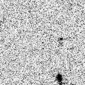
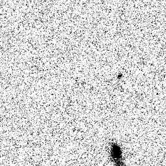
117 (a) 101 FIG. 12. (a) 10 cutouts of our 11 new objects (see F08a for a similar figure for the original four objects). The circles are 2 in diameter, and are drawn to highlight the object. The columns from left-to-right: narrowband image (NB665 or NB673 depending on the object); HST/ACS B, V, i and z ; Spitzer/IRAC 3.6, 4.5, 5.8 and 8.0 µm. All objects are easily visible in the narrowband detection images, and all look to have a brighter narrowband than V-band image by eye. All objects, except CS2-7, are undetected in the IRAC 5.8 and 8.0 µm images. The lack of detectable B-band flux illustrates the high-redshift nature of these objects. While many objects are crowded in the IRAC 3.6 and 4.5 µm images, our use of the TFIT algorithm uses the ACS z high resolution image as a template to extract the fluxes of our crowded sources.

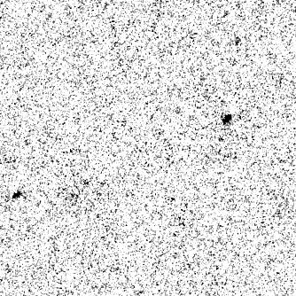
118 (b) FIG. 12. (b) Continued. 102