Constrained dynamics

Transcription

1 Constrained dynamics

2 Simple particle system In principle, you can make just about anything out of spring systems In practice, you can make just about anything as long as it s jello

3 Hard constraints

4 Constraint force Single implicit constraint Multiple implicit constraint Parametric constraint Implementation

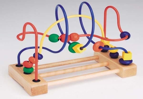
5 A simple example A bead on a wire The bead can slide freely along the wire, but cannot come off it no matter how hard you pull it. How do we simulate the motion of the bead when arbitrary forces applied to it?

6 Penalty constraints Why not use a spring to hold the bead on the wire? Problems: weak springs won t do the job strong springs give you stiff systems

7 First order world N f T In this world, f = mv ff ˆf N What is the legal velocity? What is the legal force? Add constraint force ˆf to cancel the illegal part of f f = f + ˆf ˆf = N f N N N

8 The real world N ˆf? v f a In the real world, f = ma What is the legal acceleration? depends on both N and the faster you re going, the faster you have to turn v Compute ˆf such that f only generates legal acceleration f = f + ˆf

9 Constraint force Need to compute constraint forces that cancel the illegal applied forces Which means we need to know what legal acceleration is

10 Constraint force Single implicit constraint Multiple implicit constraint Parametric constraint Implementation

11 Constraints Implicit: x C(x) = x r =0 θ r Parametric: x = r [ cos θ sin θ ]

12 Legal acceleration C =0 Ċ =0 C =0 What is the legal position? C(x) = 1 2 x x 1 2 =0 What is the legal velocity? Ċ(x) =x ẋ =0 What is the legal acceleration? C(x) =ẍ x + ẋ ẋ =0

13 Legal conditions C =0 Ċ =0 C =0 If we start with legal position and velocity C(x) =0 Ċ(x) =0 We need only ensure the legal acceleration C(x) =0

14 Constraint force Use the legal condition to compute the constraint force Rewrite the legal condition in a general form C(x) = Ċ x ẋ + C x ẍ =0 C x : constraint gradient Substitute ẍ with ẍ = f + ˆf m C = Ċ x ẋ + C x f + ˆf m =0 C x ˆf = C x f m Ċ xẋ

15 Constraint force C x ˆf = C x f m Ċ xẋ How many variables do we have? Need one more condition to solve the constraint force

16 Virtual work Constraint force is passive - no energy gain or loss Kinetic energy of the system: T = 1 2 mẋ ẋ Virtual work done by f and ˆf : T = ẋ mẍ = ẋ f + ẋ ˆf Make sure ˆf does no work for every legal velocity: ẋ ˆf =0, ẋ C x ẋ =0 Ċ(x) = C x ẋ =0

17 Constraint force ˆf ẋ ˆf =0, ẋ C x ẋ =0 must point in the direction of C x ˆf = λ C x Substituting for ˆf in C x ˆf = C x f m Ċ xẋ λ = C x f m Ċ x ẋ C x C x

18 Two conditions Legal acceleration C x ˆf = C x f m Ċ xẋ Principle of virtual work ˆf = λ C x

19 The Bead Example N v f C(x) = 1 2 x x 1 2 =0 ˆf? ˆf = λ C x λ = C x f m Ċ x ẋ C x C x

20 Feedback In principle, ensuring legal acceleration can keep the particle exactly on the circle In practice, two problems cause the particle to drift numerical errors can accumulate when the ODE is not solved exactly constraints might not be met initially

21 Feedback A feedback term handles both problems: C = k s C k d Ċ instead of C =0

22 Constraint force Single implicit constraint Multiple implicit constraint Parametric constraint Implementation

23 Tinkertoys Now we know how to simulate a bead on a wire Apply the simple idea, we can create a constrained particle system

24 Constrained particles Particles: each particle represents a point in the phase space Forces: each force affects the acceleration of certain particles Constraints: Each is a function C i (x 1, x 2,...) Legal state: C i (x 1, x 2,...)=0, i Constraint force: linear combination of constraint gradients C i x, i

25 Constraint gradients Normal of C 1 : Normal of C 2 : C 1 x C 2 x Legal states: the intersection of two planes Normal of the legal states: +

26 Implicit constraint Each constraint is represented by an implicit function What does the normal of a hypersurface mean? The direction where the particle is not allowed to move What does the intersection of the hypersurface represent? Legal state The constraint force lies in the space spanned by the constraint normals

27 Particle system notations General 3D case q Q W x 1 x 2 f 1 f 2 1 m 1 I 1 m 2 I q: 3n long position vector.... Q: 3n long force vector x n f n 1 m n I W : 3n 3n inverse mass matrix

28 Constraint notations Additional notations C λ J J C 1 C 2 λ 1 λ 2 C 1 q 1 C 1 q 2 C 1 q 3n C 2 q 1... Ċ1 q 1 Ċ2 q 1 Ċ1 q 2... Ċ1 q 3n C m λ m C m q 3n Ċm q 3n C: m long constraint vector λ: m Lagrangian multipliers J: m 3n Jacobian matrix J: time derivative of Jacobian matrix

29 Constraint equations C = Ċ x ẋ + C x ẍ C = J q + J q C = Ċ x ẋ + C x f + ˆf m =0 C = J q + JW(Q + ˆQ) =0 C x ˆf = C x f m Ċ xẋ JW ˆQ = J q JWQ C x λ C x = C x f m Ċ xẋ JWJ T λ = J q JWQ

30 Multiple force constraints To solve for force constraints, we need to solve for this linear system JWJ T λ = J q JWQ One nice property of positive definite matrix Can you prove that? JWJ T is that it is symmetric Once the linear system has been solved, the vector λ is multiplied by vector ˆQ J T to produce the global constraint force

31 Constraint force Single implicit constraint Multiple implicit constraint Parametric constraint Implementation

32 Constraints x Implicit: C(x) = x r =0 θ r Parametric: x = r [ cos θ sin θ ]

33 Parametric constraints x f x = r [ cos θ sin θ ] θ r Constraint is always met exactly 1 degree of freedom: Solve for θ

34 First order world θ x N In this world, f = mv ẋ = f + ˆf m ẋ = T θ T θ = f + ˆf m T = x θ T T θ = T f m + T ˆf m ˆf = λ C x = λn θ = 1 m T f T T

35 The real world θ x N In the real world, f = ma ẋ = T θ T = x θ ẍ = Ṫ θ + T θ = f + ˆf m T Ṫ θ + T T θ = T f m + T ˆf m θ = T f m T Ṫ θ T T

36 Particle system notations General 2D case q x 1 x 2. u θ 1 θ 2. Q f 1 f 2. m 1 I m 2 I... M q: 2n long position vector u: n long parameter vector Q: 2n long force vector x n θ n f n m n I M: 2n by 2n mass matrix

37 Constraint notations Additional notations J J q 1 q 1 u 1 u n q 2 u 1 q 1 u 1 q 2 u 1 q 1 u n J : 2n by n Jacobian matrix J : time derivative of J q 2n u 1 q 2n u n q 2n u 1 q 2n u n

38 Constraint equations ẍ = Ṫ θ + T θ = f + ˆf m T Ṫ θ + T T θ = T f m θ = T f m T Ṫ θ T T M q = M( J u + Jü) =Q + ˆQ J T M( J u + Jü) =J T Q J T MJü = J T M J u + J T Q where T = x θ where J = q u

39 Parametric vs. implicit Parametric Implicit J T MJü = J T M J u + J T Q JWJ T λ = J q JWQ where J = q u where J = C q Lagrangian dynamics

40 Parametric constraints Advantages: Fewer degrees of freedom Constraints are always met Disadvantages: Hard to formulate constraints Hard to combine constraints

41 Impress your friends The requirement that constraints not add or remove energy is called the Principle of Virtual Work The λ s are called Lagrangain Multipliers The derivative matrix J is called the Jacobian Matrix

42 Constraint force Single implicit constraint Multiple implicit constraint Parametric constraint Implementation

43 How do we implement all this? We have a global matrix equation We want to build a model on the fly Each constraint function knows how to evaluate the function itself and its various derivatives

44 How do we hook this up? We have a basic particle system which main job is to perform derivative evaluations To add constraints to the basic system, we need to modify the data structure of the basic system the deriv eval loop

45 Basic particle system system solver interface solver particles GetDim 6n n time forces Get/Set State Deriv Eval x 1 v 1 x 2 v 2 v v 1 m 1 f 1 2 f 2... m 2... x n v n v n fn m n

46 Constrained system system particles n time x 1 v 1 f 1 m 1 x 2 v 2 f 2 m 2... x n v n f n m n forces F 1 F 2... F p constraints C 1 C 2... C m

47 A Constraint C x p x q v p v q f p f q m p m q code that evaluates p j len apply_fun C Ċ C q Ċ q global structure C Ċ J J q λ ˆQ

48 Jacobian matrix n blocks Each constraint contributes one or more blocks to the Jacobian matrix m blocks C i Sparsity: many empty blocks Modularity: let each constraint compute its own blocks x j x k Constraint and particle indices determine block location

49 Deriv Eval 1. Clear force accumulators x 1 v 1 f 1 m 1 x 2 v 2 f 2 m 2... x n v n f n m n 2. Invoke apply_force functions F 1 F 2... F p 3. Return derivatives to solver [ ] [ ] ẋ v = f v m

50 Modified Deriv Eval loop 1. Clear force accumulators x 1 v 1 f 1 m 1 x 2 v 2 f 2 m 2... x n v n f n m n 2. Invoke apply_force functions F 1 F 2... F p 4. Return derivatives to solver [ ] [ ] ẋ v = f v m 3. Compute and apply constraint forces C 1 C 2... C m

51 Constraint force eval After computing ordinary forces: loop over constraints, assemble global structure call matrix solver to solve for λ, multiply by J T to get constraint force add constraint force to the force accumulator in the corresponding particle

52 What s next?

53 Beyond mass points: equations of motion for real objects Read: Constrained dynamics by Witkin and Baraff