Differential Equations

Size: px

Start display at page:

Download "Differential Equations"

Sophie Francis
5 years ago
Views:

1 Differential Equations

4 Overview of differential equation! Initial value problem! Explicit numeric methods! Implicit numeric methods! Modular implementation

5 Physics-based simulation An algorithm that produces a sequence of states over time under the laws of physics! What is a state?

6 Physics simulation x i differential equations x i+1 integrator x i x i+1 = x i + x x

7 Differential equations What is a differential equation?! It describes the relation between an unknown function and its derivatives! Ordinary differential equation (ODE)! is the relation that contains functions of only one independent variable and its derivatives

8 Ordinary differential equations An ODE is an equality equation involving a function and its derivatives known function ẋ(t) =f(x(t)) time derivative of the unknown function unknown function that evaluates the state given time What does it mean to solve an ODE?

9 Symbolic solutions Standard introductory differential equation courses focus on finding solutions analytically! Linear ODEs can be solved by integral transforms! Use DSolve[eqn,x,t] in Mathematica Differential equation: ẋ(t) = Solution: x(t) =e kt kx(t)

10 Numerical solutions In this class, we will be concerned with numerical solutions! Derivative function f is regarded as a black box! Given a numerical value x and t, the black box will return the time derivative of x

11 Physics-based simulation x i differential equations x i+1 integrator x i x i+1 = x i + x x

12 Overview of differential equation! Initial value problem! Explicit numeric methods! Implicit numeric methods! Modular implementation

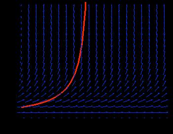
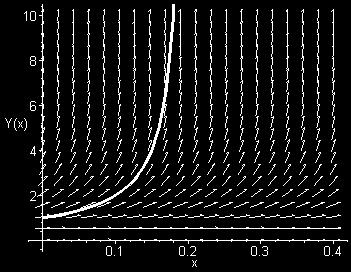
13 Initial value problems In a canonical initial value problem, the behavior of the system is described by an ODE and its initial condition: ẋ = f(x, t) x(t 0 )=x 0 To solve x(t) numerically, we start out from x 0 and follow the changes defined by f thereafter

14 Vector field x 2 The differential equation can be visualized as a vector field ẋ = f(x,t) x 1

15 Quiz Which one is the vector field of ẋ = 0.5x?

16 Vector field x 2 The differential equation can be visualized as a vector field ẋ = f(x,t) How does the vector field look like if f depends directly on time? x 1

17 Integral curves t 0 f(x,t)dt f(x,t)

18 Physics-based simulation x i Newtonian laws gravity wind gust x i+1 elastic force.. integrator x x i x i+1 = x i + x

19 Overview of differential equation! Initial value problem! Explicit numeric methods! Implicit numeric methods! Modular implementation

20 Explicit Euler method How do we get to the next state from the current state? x(t 0 + h) x(t 0 ) p x(t 0 + h) =x 0 + hẋ(t 0 ) Instead of following real integral curve, p follows a polygonal path Discrete time step h determines the errors

21 Problems of Euler method Inaccuracy The circle turns into a spiral no matter how small the step size is

22 Problems of Euler method Instability ẋ = kx Symbolic solution: x(t) =e kt Oscillation: x(t) oscillates around equilibrium. Divergence: x(t) eventually goes to infinity (or negative infinity).

23 Problems of Euler method Instability ẋ = kx Symbolic solution: x(t) =e kt h < 1/k to avoid oscillation

24 Quiz Instability ẋ = kx Symbolic solution: x(t) =e kt What s the largest time step without divergence?

25 Quiz Instability ẋ = kx Symbolic solution: x(t) =e kt What s the largest time step without oscillation?

26 Accuracy of Euler method At each step, x(t) can be written in the form of Taylor series:! is a representation of a function as an infinite sum of terms calculated using! x(t 0 + h) =x(t 0 )+hẋ(t 0 )+ h2 2! ẍ(t 0)+ h3 3! x(3) (t 0 )+... hn the n x derivatives at a particular point n! t n What is the order of the error term in Euler method?! The cost per step is determined by the number of evaluations per step

27 Stability of Euler method Assume the derivative function is linear!! Look at x parallel to the largest eigenvector of A!! Note that eigenvalue d dt x = Ax d dt x = λx λ can be complex

28 The test equation Test equation advances x by!! x n+1 = x n + hλx n Solving gives!! x n =(1+hλ) n x 0 Condition of stability 1+hλ 1

29 Stability region Plot all the values of hλ on the complex plane where Euler method is stable

30 Real eigenvalue If eigenvalue is real and negative, what kind of the motion does x correspond to?! a damping motion smoothly coming to a halt! The threshold of time step!! h 2 λ What about the imaginary axis?

31 Imaginary eigenvalue If eigenvalue is pure imaginary, Euler method is unconditionally unstable! What motion does x look like if the eigenvalue is pure imaginary?! an oscillatory or circular motion! We need to look at other methods

32 The midpoint method 1. Compute an Euler step x = hf(x(t 0 )) 2. Evaluate f at the midpoint f mid = f(x(t 0 )+ x 2 ) 3. Take a step using f mid x(t 0 + h) =x(t 0 )+hf mid x(t + h) =x 0 + hf(x 0 + h 2 f(x 0))

33 Accuracy of midpoint Prove that the midpoint method has second order accuracy x(t + h) =x 0 + hf(x 0 + h 2 f(x 0)) x = h 2 f(x 0) f(x 0 + x) =f(x 0 )+ x f(x 0) x x(t + h) =x 0 + hf(x 0 )+ h2 2 f(x 0) f(x 0) x x(t + h) =x 0 + hẋ 0 + h2 2 ẍ0 + O(h 3 ) + O(x 2 ) + ho(x 2 )

34 Stability region x n+1 = x n + hλx n+ 1 2 = x n + hλ(x n hλx n) x n+1 = x n (1 + hλ (hλ)2 ) hλ = x + iy 1 [ 0 ] + [ x y ] [ x 2 y 2 2xy ] 1 [ 1+x + x 2 y 2 2 y + xy ] 1

35 Stability of midpoint Midpoint method has larger stability region, but still unstable on the imaginary axis

36 Quiz RK2 RK1 Consider a dynamic system where = 2 i2 What is the largest time step for RK1? What is the largest time step for RK2?

37 Runge-Kutta method Runge-Kutta is a numeric method of integrating ODEs by evaluating the derivatives at a few locations to cancel out lower-order error terms! Also an explicit method: x n+1 is an explicit function of x n

38 Runge-Kutta method q-stage p-order Runge-Kutta evaluates the derivative function q times in each iteration and its approximation of the next state is correct within O(h p+1 )! What order of Runge-Kutta does midpoint method correspond to?

39 4-stage 4 th order Runge-Kutta k 1 = hf(x 0,t 0 ) k 2 = hf(x 0 + k 1 2,t 0 + h 2 ) k 3 = hf(x 0 + k 2 2,t 0 + h 2 ) k 4 = hf(x 0 + k 3,t 0 + h) x(t 0 + h) = x k k k k 4 x 1. f(x 0,t 0 ) x 0 2. f(x 0 + k 1 2,t 0 + h 2 ) f(x 0 + k ,t 0 + h 2 ) x(t 0 + h) f(x 0 + k 3,t 0 + h) t 4.

40 High order Runge-Kutta RK3 and up are include part of the imaginary axis

41 Quiz If lambda is where the red dot is, which integrators can generate stable simulation? RK1 (A) RK4 only (B) RK4 and RK3 (C) RK4, RK3, and RK1

42 Stage vs. order p q The minimum number of stages necessary for an explicit method to attain order p is still an open problem Why is fourth order the most popular Runge Kutta method?

43 Adaptive step size Ideally, we want to choose h as large as possible, but not so large as to give us big error or instability! We can vary h as we march forward in time! Step doubling! Embedding estimate! Variable step, variable order

44 Step doubling Estimate x a by taking a full Euler step x a = x 0 + hf(x 0,t 0 ) e Estimate x b by taking two half Euler steps x temp = x 0 + h 2 f(x 0,t 0 ) x b = x temp + h 2 f(x temp,t 0 + h 2 ) e = x a x b is bound by O(h 2 ) Given error tolerance ϵ, what is the optimal step size? ( ϵ e)1 2 h

45 Quiz I use step doubling at the current step and the error is 0.4. Given that the error threshold of the simulation is set at 0.001, I should (A) Increase h by 400 times! (B) Decrease h by 400 times! (C) Increase h by 20 times! (D) Decrease h by 20 times

46 Embedding estimate Also called Runge-Kutta-Fehlberg! Compare two estimates of! x(t 0 + h) Fifth order Runge-Kutta with 6 stages! Forth order Runge-Kutta with 6 stages

47 Variable step, variable order Change between methods of different order as well as step based on obtained error estimates! These methods are currently the last work in numerical integration

48 Problems of explicit methods Do not work well with stiff ODEs! Simulation blows up if the step size is too big! Simulation progresses slowly if the step size is too small

49 Example: a bead on the wire y(t) Y(t) =(x(t),y(t)) x(t) Ẏ = d dt ( x(t) y(t) ) = ( x(t) ky(t) ) Explicit Euler s method: Y new = Y 0 + hẏ(t 0)= ( x(t) y(t) ) + h ( x(t) ky(t) ) Y new = ( (1 h)x(t) (1 kh)y(t) )

50 Stiff equations Stiffness constant: k! Step size is limited by the largest k! Systems that has some big k s mixed in are called stiff system

51 Overview of differential equation! Initial value problem! Explicit numeric methods! Implicit numeric methods! Modular implementation

52 Implicit methods Explicit Euler: Y new = Y 0 + hf(y 0 ) Implicit Euler: Y new = Y 0 + hf(y new ) Solving for Y new such that! f, at time t 0 + h, points directly back at!!! Y 0

53 Implicit methods Our goal is to solve for Y new such that Y new = Y 0 + hf(y new ) Approximating f(y new ) by linearizing f(y) f(y new )=f(y 0 )+ Yf (Y 0 ), where Y = Y new Y 0 Y new = Y 0 + hf(y 0 )+h Yf (Y 0 ) ( ) 1 1 Y = h I f (Y 0 ) f(y 0 ) f(y,t)=ẏ(t) f(y,t) = f Y

54 Example: A bead on the wire Apply the implicit Euler method to the bead-on-wire example ( ) 1 1 Y = h I f (Y 0 ) f(y 0 ) [ ] x(t) f(y(t)) = ky(t) [ 1 0 f (Y(t)) = f(y(t)) = Y 0 k [ 1+h ] 1 [ ] Y = h 0 x0 1+kh 0 ky 0 = = h [ h h h 1+kh [ h h+1 x 0 h 1+kh ky 0 ] ][ ] x0 ky 0 ]

55 Example: A bead on the wire What is the largest step size the implicit Euler method can take? lim Y = lim h h [ = x 0 1 k ky 0 [ h h+1 x 0 h 1+kh ky 0 ] = ] [ x0 y 0 ] Y new = Y 0 +( Y 0 )=0

56 Quiz Consider a linear ODE in apple ẋ = f(x) = R x If h = 1 and the current state is apple What is the next state computed by an implicit integrator?

57 Stability of implicit Euler Test equation shows stable when!! 1 hλ 1 How does the stability region look like?

58 Problems of implicit Euler Implicit Euler could be stable even when physics is not!! Implicit Euler damps out motion unrealistically

59 Implicit vs. explicit correct solution: x(h) =e hk x ẋ(h) = kx(h) x(0) = 1 explicit Euler: implicit Euler: x(h) = x(h) =1 hk 1 1+hk h

60 Trapezoidal rule Take a half step of explicit Euler and a half step of implicit Euler!! x n+1 = x n + h( 1 2 f(x n)+ 1 2 f(x n+1)) Explicit Euler is under-stable, implicit Euler is over-stable, the combination is just right

61 Stability of Trapezoidal What is the test equation for Trapezoidal?!! hλ 0 Where is the stability region?! negative half-plane! Stability region is consistent with physics! Good for pure rotation

62 Terminology Explicit Euler is also called forward Euler! Implicit Euler is also called backward Euler

63 Overview of differential equation! Initial value problem! Explicit numeric methods! Implicit numeric methods! Modular implementation

64 Modular implementation Write integrator in terms of! Reusable code! Simple system implementation! Generic operations:! Get dim(x)! Get/Set x and t! Derivative evaluation at current (x, t)

65 Solver interface GetDim System (black box) Get/Set State Solver (integrator) Deriv Eval

66 Summary Explicit Euler is simple, but might not be stable; modified Euler may be a cheap alternative! RK4 allows for larger time step, but requires much more computation! Use implicit Euler for better stability, but beware of over-damp

67 Quiz When I tried to simulate an ideal spring using explicit Euler method, the simulation blew up very quickly after a few iterations. Which of the following actions will result in stable simulation? Why?!! 1. Reduce time step 2. Use midpoint method 3. Use implicit method 4. Use fourth order Runge Kutta method! 5. Use trapzoidal rule

Differential Equations

Pysics-based simulation xi Differential Equations xi+1 xi xi+1 xi + x x Pysics-based simulation xi Wat is a differential equation? Differential equations describe te relation between an unknown function