Simulation and Modification of a Composite Trombe Wall to Adapt to the Climate in Victoria, Canada
|
|
|
- Jewel Nash
- 5 years ago
- Views:
Transcription
1 Simulation and Modification of a Composite Trombe Wall to Adapt to the Climate in Victoria, Canada by Zhijie Yin BEng, Northwestern Polytechnical University, 2012 A Report Submitted in Partial Fulfillment of the Requirements for the Degree of MASTER OF ENGINEERING in the Department of Mechanical Engineering Zhijie Yin, 2016 University of Victoria All rights reserved. This report may not be reproduced in whole or in part, by photocopy or other means, without the permission of the author.
2 i Supervisory Committee Simulation and Modification of a Composite Trombe Wall to Adapt to the Climate in Victoria, Canada by Zhijie Yin BEng, Northwestern Polytechnical University, 2012 Supervisory Committee Dr. Curran Crawford Supervisor Dr. Phalguni Mukhopadhyaya Departmental Member Department of Mechanical Engineering Department of Civil Engineering
3 ii Supervisory Committee Abstract Dr. Curran Crawford Supervisor Dr. Phalguni Mukhopadhyaya Departmental Member Department of Mechanical Engineering Department of Civil Engineering As one of the passive solar techniques, the composite Trombe wall system stands out for its ability to provide better indoor thermal comfort for residents. Many experimental and numerical studies were conducted in the past to investigate its thermal performance in various climates around the world. However, no research has been done so far to adapt this passive system to Canada s west coast. In this project, an existing composite Trombe wall design is studied first with a model developed in COMSOL Multiphysics environment. After being validated with published data, this model is applied with Victoria weather conditions for both cooling and heating modes. Its insufficient heating ability for the local winter leads to a modification study. By applying the orthogonal experiment design method, two parametric simulation studies are conducted to optimize several geometric and thermal dynamic properties of the structure. Compared to the original design, the modified model achieves better indoor average temperature stability and less spatial temperature stratification. The results of this study are fundamental in helping architects or project managers to introduce this bioclimatic design to Canada s west coast.
4 iii Table of Contents Supervisory Committee... i Abstract...ii Table of Contents... iii List of Figures... v List of Tables... vii Nomenclature... viii Acknowledgement... xii Chapter 1 Introduction Overview Objectives... 3 Chapter 2 Model Development Geometric Parameters Thermal Dynamic Properties Assumptions and Boundary Conditions Thermal Resistance Network Fourier s Law for Heat Conduction in Differential Form Newton s Law of Cooling for Heat Convection Stefan-Boltzmann Law for Radiation Theoretical Calculation Energy Balance Convection Coefficients Emission Factors Meteorological Data Mesh Numerical Solver Chapter 3 Validating Model Chapter 4 Simulation for Model Evaluation... 28
5 iv 4.1 Heating Season Cooling Season Chapter 5 Trombe Wall Parametric Study Study One Selecting Orthogonal Array Wall Parameter Study Results Analysis of Variance Near Optimal Level Value and Optimal Configuration Study Two Selecting Orthogonal Array Wall Parameter Study Results Analysis of Variance Near Optimal Level Value and Optimal Configuration Demonstration of Thermal Storage Function of the Mass Wall Simulation Results Chapter 6 Conclusion and Recommendation Reference... 64
6 v List of Figures Figure 1: Trombe wall... 2 Figure 2: Composite Trombe wall... 3 Figure 3: Geometric parameters... 6 Figure 4: Schematic of boundary conditions... 9 Figure 5: Schematic of thermal resistance network for the composite Trombe wall Figure 6: Meteorological data-temperature and wind speed for Carpentras, France Figure 7: Meteorological data-solar heat flux for Carpentras, France Figure 8: Mesh quality spatial distribution Figure 9: Mesh quality statistic distribution Figure 10: Temperature at the external surface of the mass wall Figure 11: Temperature at the internal surface of the insulation wall Figure 12: Thermal profile of the wall at 08:00(a), 12:00(b), 16:00(c) Figure 13: Velocity profile of the wall at 08:00(a), 12:00(b), 16:00(c) Figure 14: Winter meteorological data-temperature and wind speed for Victoria, Canada Figure 15: Winter meteorological data-solar radiation for Victoria, Canada Figure 16: Time dependent temperature distribution within the wall Figure 17: Average air temperature in the room under the influence of vents in winter Figure 18: Summer meteorological data-temperature and wind speed for Victoria, Canada.. 32 Figure 19: Summer meteorological data-solar radiation for Victoria, Canada Figure 20: Schematic of exterior vents for summer Figure 21: Average air temperature in the room under the influence of interior and exterior vents in summer Figure 22: Study 1 Average indoor temperature generated from the optimized model, compared with two cases from OA trial Figure 23: Study 2 - Indoor air temperature gradient between 0.1m and 0.7m during the last day of the optimized model from study one Figure 24: Study 2 - Indoor air temperature gradient between 0.1m and 0.7m during the last day of the optimized model from study two Figure 25: Study 2 - Time at 00:00. Magnitude of velocity (a) and temperature distribution map (b)... 52
7 vi Figure 26: Study 2 - Time at 08:00. Magnitude of velocity (a) and temperature distribution map (b) Figure 27: Study 2 - Time at 16:00. Magnitude of velocity (a) and temperature distribution map (b) Figure 28: Study 2 - Time at 24:00. Magnitude of velocity (a) and temperature distribution map (b) Figure 29: Demonstration of the passive heating and thermal storage function of the mass wall with the results from Study 2. Temperature field in mass wall at 00:00 (a); 04:00 (b); 08:00 (c); 12:00 (d); 16:00 (e); 20:00 (f); 24:00 (g)... 60
8 vii List of Tables Table 1.Geometric parameter list... 5 Table 2.Thermal physical property list... 6 Table 3.Study 1 - Selected process parameters and respective levels in the experimental design Table 4.Study 1 - Experimental layout by L9(3 4 ) OA design Table 5.Study 1 - Experimental layout with the variables in their original units Table 6.Study 1 - Performance parameter results from simulations Table 7.Study 1 - Mean values of each level for the four design factors Table 8.Study 1 - Sum of square value and percentage contribution for the four design factors Table 9.Study 1 Near optimal level value for the four design factors Table 10.Study 1 - Mean sum of square value, mean sum of square of error and weight for each factor Table 11.Study 2 - Selected process parameters and respective levels in the experimental design Table 12.Study 2 - Experimental layout by L6(3 3 ) OA design Table 13.Study 2 - Experimental layout with the variables in their original units Table 14.Study 2 - Performance parameter results from simulations Table 15.Study 2 - Mean values of each level for the design factors Table 16.Study 2 - Sum of square value and percentage contribution for the design factors.. 49 Table 17.Study 2 Near optimal level value for the design factors Table 18.Study 2 - Mean sum of square value, mean sum of square of error and weight for the design factors Table 19.Summary of both parameters studies... 60
9 viii Nomenclature Acronyms ANOVA MSE MSV NOLV PC SSV TSS Analysis of variance Mean sum of square of error Mean sum of square value Near optimal level value Percentage contribution Sum of square value Total sum of square Symbols a Thermal diffusivity m²/s A Area m² C Specific heat capacity J/kg C d F e Discharge coefficient Emission factor between two parallel surfaces F z Buoyancy force N g Acceleration of gravity m/s² Gr Grashof number h Convection coefficient W/m² C H Height m K Number of factors L Thickness m
10 ix l Le Characteristic length Number of level m Air mass flow rate kg/s M N Nu P Pr R R A Ra S Mean value of each level of a design factor Number of experiments conducted Nusselt number Performance parameter value Prandtl number Thermal resistance Specific gas constant Rayleigh number Sum of observations of all experiments T Temperature K v velocity m/s W Width m x Cartesian coordinate Greek letters Φ Heat flux kj/h β Volumetric thermal expansion coefficient 1/K ε ζ Emissivity Sum of load loss coefficients λ Thermal conductivity W/m C μ Dynamic viscosity Pa s
11 x ρ Density kg/m³ σ Stefan Boltzmann constant E-8 W/m² K⁴ τ ϒ Transmissivity Ratio of specific thermal capacity φ Heat flux density W/m² δ Tiny length element m ω Weight for each factor Subscripts amb avg bottom ch close cond conv env f fl g gy i in m Ambiance Average Bottom vent Chimney Vent closed Conduction Convection Environment Fluid Floor Glazing Gypsum Insulation Inside surface Mass wall
12 xi open out r ra s top v w Vent open Outside surface Interior room Radiation Solar Top vent Vent Wind
13 xii Acknowledgement I would first like to thank my supervisor, Dr. Curran Crawford, for always being patient and supportive whenever I had questions about my research project. As well a heartfelt thank you to the Sustainable System Design Lab group for all the knowledge and fun experiences in and out of the lab. I would also like to acknowledge my friend Ken Streutker for providing me valuable assistance with writing skills in my second language, English. Finally, I must express my gratitude to my parents and my partner for providing me with unfailing support and continuous encouragement throughout my years of study. Zhijie Yin
14 1 Chapter 1 Introduction 1.1 Overview With passive solar techniques, it is possible to reduce the annual heating and cooling demand of buildings so they meet the passive house standard. According to the Passive House Institute, for a building to be considered a passive house, the space heating energy demand should not exceed 15 kwh per square meter per year. [1]. For different climate regions, the passive house principle remains the same, while the specific solution has to be adapted to the region. Among various passive solar systems developed to make use of solar thermal energy, such as solar chimneys [2], solar roofs [3], etcetera, the Trombe wall system stands out for its high efficiency [4] in heating building interiors in the winter time. A Trombe wall, as shown in Figure 1, is a passive solar building design: a wall is built on the winter sun side of a building with a glass external layer and a high heat capacity internal layer separated by a layer of air [5]. The black surface of the high mass wall absorbs solar energy and heats up. The gained heat is stored in the wall and conducted into the adjacent interior space throughout the day and night. The idea of the Trombe wall is similar to the design of south-facing windows combined with mass floor. Compared to the latter one, the main advantage of Trombe wall is its simplicity and ability to provide better indoor comfort level, as it separates the energy gathering surface from living space. However, it can suffer large heat loss during the night or on cloudy days, or produce excessive heat in the summer time due to its low thermal resistance. Once the stored energy in the mass wall is depleted, a reverse heat flow begins from inside to the outside leading to heat loss from the dwelling.
15 2 Figure 1: Trombe wall A solution is to include an insulation panel located at the back of the mass wall. This composite system is called the Trombe-Michel wall [6] as shown in Figure 2. On sunny days, the gained energy in the mass wall is exchanged by convection with the air layer between the mass wall and the insulation panel. Natural circulation occurs in the air gap through buoyancy. The room air is admitted through a lower vent, heated up by convection in the chimney, and discharged back to the room through an upper vent. Meanwhile, the heated insulation wall transfers the remaining heat to the interior by conduction. On cloudy days or at night, the upper and lower vents in the insulating wall are both closed, forming a thermal barrier with the insulating wall to reduce both reverse heat circulation and heat flux going from indoor to outdoor. Due to the presence of the insulating wall, the air layer and the vents, the composite Trombe wall has several advantages over the classical Trombe wall. It has better heat resistance to keep heat inside in the winter time and avoid overheating in the summer time. Besides, the heat supply can also be controlled by adjusting the air vents.

16 3 Figure 2: Composite Trombe wall In this research, the finite element method tool, COMSOL Multiphysics 5.1 was used to simulate the heat transfer that occurs in the composite Trombe wall system to optimize the temperature field in the interior space. COMSOL Multiphysics is a FEA simulation software package for various physics and engineering applications, especially for multi-physics. The heat transfer module and the fluid flow module were applied in this project to develop the time dependent model. In the simulation phase, COMSOL s parametric sweep function made it more efficient to conduct multi-factor involved parametric study. 1.2 Objectives Many experimental structures and numerical models were created for the composite Trombe wall study, but so far no research has been done to adapt this passive heating and cooling system to Canada s west coast. Due to its special climate conditions with mild cloudy winters, it is worth investigating whether the composite Trombe wall will perform well in this location. This work aims at establishing a clear numerical methodology to quantify the thermal performance of the system and modifying an existing model to achieve indoor thermal comfort with local Victoria, B.C. weather conditions. The objective is to provide guidance for optimizing the passive system generally and understand how different parameters impact the
17 4 performance of the system. The research described in this study is comprised of the following activities. Creation of a numerical model to simulate the composite Trombe wall performance. Validation of numerical simulation using published results. Simulation with the original model and Victoria s weather data to evaluate its performance locally. Modification of the original model with a two-step parametric design study.
18 5 Chapter 2 Model Development This study is based on Zalewski and his team s research [7]. A measurement experiment was carried out on site in Cadarache, southern France with local weather data. Several simulation studies based on the same wall structure were performed in the following years. [8] - [10]. The same geometric and thermal dynamic parameters of the composite Trombe wall were adopted in this study. Zalewski s simulation model was developed in one dimension as the original research was focused on the thermal performance of the wall with indoor air temperature simplified as one constant value. In this research, the goal is to study the temperature distribution in the dwelling space and create a thermal comfort environment with minimum temperature stratification. Considering the high calculation cost of a 3D model, and the structure characteristics, a 2D finite element model will be developed for the study. 2.1 Geometric Parameters The geometric parameters are listed in Table 1 and illustrated in Figure 3. Table 1.Geometric parameter list Geometric Parameters Wall height H 2.47 m Wall width W 1.34 m Glass thickness L g m Interval between the glazing and the mass wall L m Mass wall thickness L m 0.15 m Interval between the mass wall and the insulating wall L m Height of the orifices of the insulating wall H v 0.15 m Width of the orifice of the insulating wall W v 0.6 m Vertical distance between two orifices H 0 2 m Insulating wall thickness L i m Gypsum thickness L gy 0.01 m Room length L r 3.15 m Vent distance to the floor or ceiling H fl m
19 6 Figure 3: Geometric parameters 2.2 Thermal Dynamic Properties Most of thermal dynamic properties of each material were referred from the previous simulation models. [8] As to the parameter values of glazing, values are adopted based on the assumption that the glazing is double-paned with conductivity as 0.69 W/m, glass density as 2210 kg/m 3 and glass heat capacity as 800 J/kg [11]. All the material thermal physical properties are assumed to be independent of temperature, as shown in Table 2. Table 2.Thermal physical property list Material Properties Emissivity Conductivity Density Heat Capacity Transmissivity (ε) λ (W/m ) ρ (kg/m 3 ) C (J/kg ) τ Glazing ε g 0.9 λ g 0.69 ρ g 2210 C g 800 τ g 0.81 Mass wall ε m 0.9 λ m 0.81 ρ m 1900 C m 949 Insulating wall ε i 0.6 λ i ρ i 30 C i 800 Gypsum ε gy 0.9 λ gy ρ gy 1000 C gy 800
20 7 As this passive solar thermal system involves natural convection, the air properties are assumed to be functions of temperature. According to John C. Dixon [12], the following air thermal physical properties are formulated: The thermal conductivity λ is given by where T K is the absolute temperature T K λ = T K /T K W (2.1) m K The specific thermal capacity c p at constant pressure is given by the empirical expression c p = (T K 200) 2 J kg K (2.2) The specific heat at constant volume c V is then where R A is the specific gas constant c V = c p R A (2.3) The ratio of specific thermal capacity γ is R A = J kg K (2.4) The dynamic viscosity μ is given by γ = c p c V (2.5) μ = T K 1.5 T K Pa s (2.6) The volumetric thermal expansion coefficient of air at constant pressure is given by β = 1 T K (2.7)
21 8 2.3 Assumptions and Boundary Conditions Before processing heat transfer calculations, the following assumptions are made to simplify the model: The width of the wall structure is large enough compared with the thickness. As a result, it is taken as a two-dimensional configuration in x-z plain. The top and bottom wall surfaces are well insulated. Moreover, the heat transfer is only in the form of radiation and conduction for the air gap between the glazing and the mass wall to simplify the calculation. Therefore, heat transfer is one dimensional in the wall. The only temperature gradient exists in the horizontal direction. The heat transfer through the glazing and wall is time dependent. All surfaces are treated as grey bodies with diffuse reflection and emission. Except for the air, all the material thermal physical properties are independent of temperature. Air is considered as a nonparticipating medium in radiation heat transfer. Air is considered as Newton flow. Flow in the system is all laminar flow. The schematic in Figure 4 shows the applied boundary conditions in different colours. To simplify the model, the horizontal boundaries were set as insulation (black, except the room floor). Ground temperature was applied to the interior room s floor (orange). The exterior surface of the glazing was exposed to both convective heat flux and solar radiation (red). On the internal boundaries presented in magenta, surface-to-surface radiation condition was applied in order to simulate greenhouse effect. The remaining internal boundaries were set as continuity (grey).
22 9 Figure 4: Schematic of boundary conditions 2.4 Thermal Resistance Network To better understand the general behavior of the composite Trombe wall and identify those design factors that are most critical, the thermal resistance network technique is applied here. It is an electrical analogy of the method used in electrical engineering to analyze the voltage in a circuit. The analog of φ is current, and the analog of the temperature difference ΔT is voltage difference and R is the thermal resistance. φ = ΔT R The analysis is based on the idea that a system consists of different discrete points, knowns as nodes, which are interconnected by the thermal resistance in between. At the boundary, external heat influx and reference temperatures are applied to the relevant nodes. Within the network, the thermal path between two nodes is assumed as one-dimensional. By applying energy balance on each node, the related temperature can be calculated. The equations used are the fundamental heat transfer equations for conduction, convection, and radiation with unit area respectively. The thermal resistances are derived at using the following equations: (2.8)
23 Fourier s Law for Heat Conduction in Differential Form φ = λ dt dx where λ is thermal conductivity of the material between the nodes (W (m K) ), dt is the dx temperature gradient. For a simpler form for the thermal resistance, (2.9) φ = λ T 1 T 2 l = T 1 T 2 l λ (2.10) let R cond = l λ where l is the distance between nodes Newton s Law of Cooling for Heat Convection φ = h(t 1 T 2 ) = T 1 T 2 1 h where h is the heat transfer coefficient of the solid node (W m 2 K), define R conv = 1 h (2.11) (2.12) Stefan-Boltzmann Law for Radiation φ = εσ(t 4 1 T 4 2 ) (2.13) where ε is the emissivity of the solid body surface which varies from 0 to 1; σ is called the Stefan-Boltzmann constant of which the value is W/(m 2 K 4 ). Both T 1 and T 2 are absolute temperature. The correlated thermal resistance of surface radiation is derived from below: φ = εσ(t 1 4 T 2 4 ) = T 1 T 2 1 εσ(t 1 + T 2 )(T 1 2 T 2 2 ) (2.14)
24 11 R radiation = 1 1 = h ra εσ(t 1 + T 2 )(T 2 1 T 2 2 ) where h ra is defined as radiative heat transfer coefficient. (2.15) Based on the above assumptions and analogs, a thermal resistance network for the composite Trombe wall is created as demonstrated in Figure 5. Figure 5: Schematic of thermal resistance network for the composite Trombe wall As mentioned in the assumption section, the thermal transfer in the wall exists only in horizontal direction. When the upper and lower vents are closed, the network of the wall is a one dimensional model. The inner surface of the gypsum panel is the boundary between the 1D wall model and 2D dwelling space model. When the vents are open, the boundary becomes the inner surface of the mass wall. This network helps to set up a meaningful finite element model at the early design stage. From the ambiance at the left, to the interior room on the right, heat transfers and distributes by natural convection, conduction and radiation. In the next section, each step of the heat transfer will be investigated in detail.
25 Theoretical Calculation Based on the above assumptions and thermal resistance network, the heat transfer through the composite Trombe wall is analyzed in the following steps Energy Balance From the exterior glazing surface to the interior insulation wall s gypsum surface, the energy balance equations include radiation, convection and conduction. The related convection coefficients and emission factors will be calculated in the next sections Glazing layer The thermal balance on the glazing is given by 4 φ = h gout (T amb T g ) + σfe gout.amb (T env T 4 g ) + φ sg (2.16) = h gin.f1 (T g T f1 ) + σfe gin.mout (T 4 4 g T mout ) where h gout is the convention coefficient on the exterior surface of the glazing, T amb is the air ambient temperature, Fe gout.amb is the emission factors for the outside surface of glazing, T env is the environment temperature, φ sg is the solar flux absorbed by the glass, h gin.f1 is the convention coefficient on the interior surface of the glazing, T f1 is the temperature at the midpoint of the sealed air gap, Fe gin.mout is the emission factor between the inside surface of glazing and the outside surface of the mass wall Mass wall The thermal flux through the mass wall is governed by the one-dimensional conduction heat transfer equation: T t = a 2 T m x 2 (0 < x < L m) where t is time, a m is the diffusivity of the mass wall: (2.17)
26 13 a m = λ m ρ m C pm (0 < x < L m ) (2.18) where L m is the thickness of the mass wall. The boundary conditions are given by the energy balance equation at two surfaces (x=0, x=l m ) At the exterior mass wall surface where x=0, the equation is: T λ m x 4 4 x=0 = h mout.f1 (T f1 T mout ) + σfe gin.mout (T gin T mout ) + φ sm where h mout.f1 is the convention coefficient on the exterior surface of the mass wall; φ sm is the solar heat flux absorbed by the mass wall surface. At the interior mass wall surface where x=l m, two cases are studied. (2.19) Vent open: The energy balance equation at the interior wall surface is given by: T λ m x 4 4 x=l m = h min.f2.open (T min T f2 ) + σfe min.iout (T min T iout ) where T f2 is the temperature of the air in the chimney between the mass wall and the (2.20) insulation wall; h min.f2.open is the convention coefficient on the interior surface of the mass wall with open vents; Fe min.iout is the emission factors between the inside surface of the mass wall and the outside surface of the insulating wall. Vent closed: T λ m x 4 4 x=l m = h min.f2.close (T min T f2 ) + σfe min.iout (T min T iout ) where h min.f2.close is the convention coefficient on the interior surface of the mass wall with closed vents Air chimney between the mass wall and the insulation wall In the case of open vents, a thermal circulation of air through the chimney is generated when the average air temperature in the chimney is higher than the indoor temperature. (2.21)
27 14 The thermal energy transferred to the air is given by: h min.f2 (T min T f2 ) = h iout.f2 (T f2 T iout ) + φ ch (2.22) where h iout.f2 is the convection coefficient on the outside surface of the insulating wall; T f2 is the average temperature of the air flow in the chimney. By assuming that the air temperature varies linearly along the wall height, T f2 is given by: T f2 = T vtop + T vbottom 2 where T vtop is the air outlet temperature from the chimney; T vbottom is the dwelling air (2.23) temperature at the bottom vent. On the right hand side of energy balance equation, φ ch is the thermal energy transported by the air towards the upper vent, determined by φ ch = mc f2(t vtop T vbottom ) A m (2.24) where A m is the mass wall area, m is the air mass flow rate, given by: m = ρ f2 A v v f2 (2.25) where A v is the vent area, v f2 is the average speed of the air mass flow in the chimney, given by Equation (2.26) [13] v f2 = C d gh(t vtop T vbottom ) T vtop + T vbottom (2.26) where g is the acceleration of gravity, H is the vertical distance between two vents, C d is the discharge coefficient, determined by C d = 2 (2.27) ζ ζ is the sum of load loss coefficients. Assuming that the friction losses are mostly due to the flow through the vents located at the top and bottom, ζ is given by Equation (2.28)
28 15 ζ = ζ bottom ρ f2 ( A ch ) 2 ρ f2 + ζ ρ vbottom A top ( A ch ) 2 v ρ vtop A v (2.28) where A ch is the chimney section area, ρ vbottom and ρ vtop are the air density at the average temperature T vbottom at the bottom vent and T vtop at the upper vent respectively; ζ bottom and ζ top are the load loss coefficients at the bottom and top vent respectively. According to the 2001 ASHRAE Handbook [14], when air flows from room to vent, the loss coefficient ζ bottom = 0.5 (2.29) when air flows from vent to room (abrupt exit), the loss coefficient ζ top = 1 (2.30) Insulation wall The thermal flux through the insulation wall is governed by the one-dimensional conduction heat transfer equation T t = a 2 T i x 2 (0 < x < L i) where a i is the diffusivity of the insulation wall: a i = λ i ρ i C pi (0 < x < L i ) (2.31) (2.32) where L i is the thickness of the insulation wall. The boundary conditions are given by the energy balance equation at two surfaces (x=0, x=l i ) At x=0, two cases are studied. Vent open: The energy balance equation at the exterior insulation surface is given by: T λ i x 4 4 x=0 = h iout.f2.open (T iout T f2 ) + σfe min.iout (T iout T min ) Vent closed: (2.33)
29 16 The energy balance equation at the exterior insulation surface is given by: T λ i x 4 4 x=0 = h iout.f2.close (T iout T f2 ) + σfe min.iout (T iout T min ) At x=l i, this is the interface between the insulation wall and gypsum layer, (2.34) T t = a 2 T igy x 2 ( δx < x < δx) (2.35) where a igy is the average diffusivity of the insulation material and the gypsum, δx is a tiny length element Gypsum layer T t = a 2 T gy x 2 (0 < x < L gy) where a gy is the diffusivity of the gypsum layer, a gy = λ gy ρ gy C pgy (0 < x < L gy ) (2.36) (2.37) The boundary condition at the inner surface of gypsum is given by the energy balance equation: T λ gy x 4 4 x=l gy = h gyin (T gyin T r ) + σfe gy.r (T gyin T env.r ) where h gyin is the convection coefficient on the inside surface of the gypsum panel; Fe gy.r is the emission factor between the inside surface of the gypsum panel and the interior room Convection in the dwelling area The governing equations for the convection heat transfer in the room are mass, momentum and energy conservation equations in two dimensions. (2.38) Dρ t + (ρu) x + (ρv) = 0 z ρ ( u u u + u + v t x z ) = F x p x + u μ( 2 x u z 2) ρ ( v v v + u + v t x z ) = F z p z + v μ( 2 x v z 2) (2.39)
30 17 T T T + u + v t x z = λ ( 2 T ρc p x T z 2) where F z in the momentum equation is the buoyancy force, μ is the dynamic viscosity Convection Coefficients Outside surface of the glazing h gout The average convection coefficient due to wind on the glazing [15]: h gout = v w (2.40) where v w is the wind speed gained from local meteorological data files Inside surface of the glazingh gin.f1, outside surface of the mass wall h mout.f1 In this case, heat transfers by natural convection across vertical air layer in an enclosed space formed by the inside surface of glazing, the outside surface of the mass wall and the two ends. Suppose the heat transferred by convection is Φ, the temperature difference between the two walls is ΔT 1, the temperature difference between the wall surface and the fluid in ΔT 2. Based on energy conservation, Φ = h gin.mout ΔT 1 = h gin.f1 ΔT 2 (2.41) Neglecting the slight differences between h gin.f1 and h mout.f1, the mid-fluid must be at a temperature midway between that of the two surfaces. Therefore, and ΔT 1 = 2 ΔT 2 (2.42) h gin.mout = 1 2 h gin.f1 = 1 2 h mout.f1 (2.43) where h gin.f1 is given by
31 18 h gin.f1 = Nuλ f1 L f1 (2.44) where L f1 is the thickness of the enclosed air gap, Nu is the Nusselt number. The temperatures of the inside glazing surface T gin, and the outside mass wall surface T mout are assumed to be uniform respectively, and the z = 0 and z = H ends to be insulated. The average temperature of the fluid: T f1 = T gin + T mout 2 is the characteristic temperature for the Nusselt number Nu, which is determined from [16]: (2.45) 1 Nu = Max{1, 0.288Ra 4 1 l, 0.039Ra 3 l } (2.46) where the characteristic length, l, is the distance between parallel surfaces L f1. Ra is Rayleigh number, where Gr is Grashof number, given by: Ra = GrPr (2.47) Gr = β f1gρ 2 f1 L 3 f1 (T mout T f1 ) μ 2 (2.48) Pr is Prandtl number, given by: Pr = μc f1 λ f1 (2.49) Within the chimneyh min.f2, h iout.f2 and h min.iout Vents open In the case of open vents, the chimney is an air channel. There will be fluid flow and thermal transfer in vertical direction, which means the model from this point switches to two dimension. The convection coefficients are the average value for each surface. The correlated convection coefficients are given by:
32 19 h min.f2.open = h iout.f2.open = Nuλ f2 H where the characteristic length is the wall height and the Nusselt number is determined by Equation (2.51) [17]: The Grashof number is given by: (2.50) Nu = 0.12 Pr 1 3 Gr 1 3 (2.51) Gr = β f2gρ 2 f2 H 3 (T vtop T vbottom ) μ 2 (2.52) Vents closed In the case of closed vents, as mentioned in the assumption section, the buoyancy driven flow in the narrow air gap is neglectable. Therefore, the model in this area is still one dimensional. Same as the case of h gin.mout, h min.iout is given by: h min.iout = 1 2 h min.f2.close = 1 2 h iout.f2.close (2.53) where h min.f2.close = Nuλ f2 L f2 (2.54) where the characteristic length L f2 is the thickness of the channel. Rayleigh number, Where 1 Nu = Max{1, 0.288Ra 4 1 l, 0.039Ra 3 l } (2.55) Ra = GrPr (2.56) Gr = β f2gρ 2 f2 L 3 f2 (T min T f2 ) μ 2 (2.57) Pr = μc f2 λ f2 (2.58)
33 Inside surface of the gypsum wall h gy Compared to the chimney channel, the room is an infinite space. Therefore, the coefficient for the natural convection is determined by [18]: where Nu H = 0.59(Gr H Pr) < Gr H < Nu H = (Gr H Pr) < Gr H < Nu H = 0.11(Gr H Pr) 1 3 Gr H > (2.59) Gr H = β frgρ 2 fr H 3 (T gy T r ) μ 2 (2.60) Pr = μc fr λ fr (2.61) Emission Factors For any two parallel surfaces n and m, the emission factor Fe n,m is 1 Fe n,m = 1 ε + 1 n ε 1 m where ε n and ε m are surface emissivity for n and m respectively. (2.62) 2. 6 Meteorological Data To validate the model, weather data from Carpentras in southern France (latitude N, longitude 5.03 E) is used. The validation simulation was carried out for 48 hours in February. Figure 6 and Figure 7 show the meteorological data in France.
34 Heat Flux (W/m²) Temperature( C) 21 Ambient Temperature ( C) Wind Speed (m/s) Time (h) Wind speed (m/s) Figure 6: Meteorological data-temperature and wind speed for Carpentras, France Horizontal Solar Radiation (W/m²) Time (h) Figure 7: Meteorological data-solar heat flux for Carpentras, France 2.7 Mesh The structured, non-uniform triangle mesh is generated in COMSOL Multiphysics 5.1 for validation and numerical simulation. The complete mesh consists of elements. The quality of the mesh is evaluated before the simulation. The value of the mesh element quality

35 22 is based on the ratio of the inscribed and circumscribed circles radii for the simplex corresponding to each corner of the element. [19] It ranges between 0 and 1, where 0 means a degenerated element and 1 represents the best possible element. Based on the evaluation of the mesh generated for this model, the average mesh element quality is 0.73 with the minimum element quality value of Figure 8 shows the mesh and its quality distribution in the 2D model. Figure 8: Mesh quality spatial distribution Figure 9 shows the mesh quality statistically. Less than 8% of the elements have a value lower than 0.1. Usually the value of minimum element quality is preferred greater than 0.1 [20]. In this case, the minimum value of 0.05 generated is due to the boundary layer next to the vertical inside walls which consist of long rectangular elements, leading to a relatively smaller ratio of the inscribed and circumscribed circles radii. Besides the boundary layers, the rest of the elements have really good mesh quality.
36 23 14% 12% 10% 8% 6% 4% 2% 0% Element quality Figure 9: Mesh quality statistic distribution 2.8 Numerical Solver As this model is a time dependent study, a time-dependent solver is used. In COMSOL, the implicit time-dependent solver is used to solve the ordinary differential equations (ODE). It applies variable-order variable-step-size backward differentiation formulas (BDF). BDF methods have been used for a long time and are known for their stability [19].
37 24 Chapter 3 Validating Model The model is generated based on Dr. Zalewski s papers. In order to validate this 2D model, the indoor temperature is set to 19 C throughout the simulation, same setting as the published model [9]. The geometries, material properties, boundary conditions and weather files are set identically to the published model. The COMSOL simulation results are compared with the published results gained by both experimental and numerical studies. In the structure, the external surface of the mass wall is where the most solar radiation is captured, while the internal surface of the insulation wall is where the input heat goes into the dwelling space. Therefore, temperature probes are placed on these two surfaces to compare with Zalewski s results. In some other literatures [8] [9], the thermal flux through the wall is also computed. For the sake of clarity, the simulation has been limited to 2 days. According to Zalewski, weather data of February 26 th and 27 th are used. To minimize the transient effect due to the initial conditions, before starting the simulation, two pre-run simulations with the first day s weather data are conducted. Figure 10 and Figure 11 show the temperature at the external surface of the mass wall and the internal surface of the insulation wall respectively. The shade area in the plot indicates the night hours (without solar radiation). The results show that good agreement between the COMSOL model and the published model is achieved. The deviation between the mass wall outside surface temperature is less than 3.4% with 2.05 C maximum difference at the 37 th hour and the maximum deviation for the inside insulation wall is less than 0.03% with 0.06 C maximum difference at the 32 nd hour. COMSOL modeling doesn t allow setting value to the transmissivity of glazing. The extra solar radiation which should have been absorbed and reflected by glazing is absorbed by the mass wall. This may cause the slightly higher wall temperature in its model.
38 Temperature ( C) Temperature (⁰C) 25 T_outmasswall from model (⁰C) T_outmasswall from published data (⁰C) Time (h) Figure 10: Temperature at the external surface of the mass wall T_ininsulwall from model (⁰C) T_ininsulwall from published data (⁰C) Time (h) Figure 11: Temperature at the internal surface of the insulation wall For a visual check on the model validity, the thermal and velocity profiles of the structure at 08:00, 12:00 and 16:00 are shown in Figure 12 and Figure 13 respectively. Since COMSOL doesn t allow setting a domain volumn at a constant single temeprature value, the room space at 19 C is represented by an open boundary wall close to insulation wall at 19 C on the right
 (b) (c) Figure 12: Thermal profile of the wall at 08:00(a), 12:00(b), 16:00(c) In Figure 12, solar heat collecting and thermal storage function of the Trombe wall is demonstrated.")

39 26 end. In each plot, from left (the ambience) to right (the dwelling space), the layers are glazing, sealed air gap, mass wall, air channel, insulation wall with vents, room space. (a) (b) (c) Figure 12: Thermal profile of the wall at 08:00(a), 12:00(b), 16:00(c) In Figure 12, solar heat collecting and thermal storage function of the Trombe wall is demonstrated. At 8:00, the exterior surface of the mass wall heats up first with the morning sun and the wall starts charging. During the day, its temperature keeps rising while heat travels into the room. At 16:00, the mass wall is fully charged and the air in the channel keeps transfering heat into the room. The corelated air flow velocity profiles are shown in Figure 13. Both the thermal map and the buoyancy driven flow through the vents confirms the validity of the model.


,")
40 27 (a) (b) (c) Figure 13: Velocity profile of the wall at 08:00(a), 12:00(b), 16:00(c)
41 28 Chapter 4 Simulation for Model Evaluation Based on the validated model, the performance of the composite Trombe wall will be evaluated with the weather data from Victoria, Canada. Accordingly, the model will be modified to achieve the best dwelling living condition under the local climate. Victoria has a mild warm Mediterranean climate with rainy winters and sunny summers [21]. The average daily high and low temperatures in winter are 8 C and 4 C respectively. The summer average high temperature is 20 C and low of 11 C. As the second sunniest city in British Columbia, Victoria has an average of 2,193 hours of bright sunshine annually [22]. These climate conditions make it possible to adopt composite Trombe walls in this area to reduce building energy consumption. In order to decide the structure s heating and cooling ability, the typical weather data of winter solstice day (22 nd December) and summer solstice day (21 st June) is chosen. Considering the structural thermal delay phenomenon, the day before and after the solstice days are added. These weather data of a typical meteorological year is generated based on the past ten years weather record, provided by Weather Analytics. 4.1 Heating Season Figure 14 and Figure 15 show the winter weather data (December 21-23) for heating season simulation. Within the three days, the ambient temperature ranges from 1 C to 8 C with fairly low solar radiation during the day and higher wind speed at night.
42 Heat Flux (W/m²) Temperature (⁰C) 29 Ambient Temperature (⁰C) Wind Speed (m/s) Time (h) Wind Speed (m/s) Figure 14: Winter meteorological data-temperature and wind speed for Victoria, Canada Horizontal Solar Radiation (W/m²) Time (h) Figure 15: Winter meteorological data-solar radiation for Victoria, Canada To explain how the composite Trombe wall works in the heating season, a simulation with the above weather data was carried out for a closer look at this system. Figure 16 shows the time dependent temperature distribution in the wall. The shade area in the plot indicates the night hours (without solar radiation). At 9 a.m. on December 21 st, once the sun comes out, the exterior glazing starts gaining solar heat immediately, while the Trombe wall is still in a warm-up stage. Around 11 a.m., the accumulated heat in the wall gets saturated and there is heat flux going through the inner surface of the mass wall, which leads to the temperature rise on that surface. At 1p.m., the atmosphere solar radiation comes to its peak value when the
43 Temperature ( C) 30 Trombe wall is still taking in heat until it reaches the highest value at 1:30. After the peak point, solar radiation goes down while the Trombe wall discharges. Heat flux into the interior continues even after sunset at 5 p.m. The room temperature hits the highest point at 8:30 in the evening. This discharging process provides heat to the living space until the next morning when the sun rises again. T_mass wall outside T_mass wall inside T_room Time (h) Figure 16: Time dependent temperature distribution within the wall With the composite Trombe wall passive heating during the day and the mass wall s thermal storage ability, the indoor average air temperature rises to between 17 C and 21 C, as shown in Figure 16.
44 Temperature ( C) 31 Inner vents controlled case Inner vents open case Inner vents closed case Ambient Temperature (⁰C) Time (h) Figure 17: Average air temperature in the room under the influence of vents in winter One of the advantages of the composite Trombe wall is that its vents on the interior insulation panel can be closed at night to prevent reverse air circulation. Figure 17 shows the effect of the vents on the indoor air average temperature(t r ). The shade area in the plot indicates the night hours (without solar radiation). With open vents, T r fluctuates between 14.7 C and 21.2 C. According to the West Midlands Public Health Observatory, the adequate level of wintertime warmth is 18.5 C with 22 C as a maximum comfortable room temperature for sedentary adults [23]. In this case, there are 34.8 hours out of 72 hours where T r is lower than 18.5 C. In the case of closed vents, T r has much less fluctuation with a minimum temperature of 16.5 C and a maximum of 19.8 C. The number of hours below 18.5 C drops to 29.8 hours. With controlled vents, the vents will be closed once there is reversed flow. Heat will be blocked inside and prevented from leaking when T r is higher than the wall temperature. This results in only 18.3 hours out of three days when T r is below 18.5 C. If more heat gained
45 Temperature (⁰C) 32 during the day transfers into the interior, instead of losing to the ambiance through the glazing, the number of hours when T r is lower than 18.5 C will be further reduced. This indicates that the model from the published research, which is based on the climate of France, doesn t perform as well in Victoria s climate. Structural optimization is required to make the wall achieve better interior comfort level. 4.2 Cooling Season Figure 18 and Figure 19 show the summer weather data (June 20-22) for cooling season simulation. Within these three days, the ambient temperature ranges from 14 C to 24.5 C with abundant solar radiation, which may lead to over-heating during the day. Ambient Temperature (⁰C) Wind Speed (m/s) Wind Speed (m/s) Time (h) Figure 18: Summer meteorological data-temperature and wind speed for Victoria, Canada
46 Heat Flux (W/m²) Horizontal Solar Radiation (W/m²) Time (h) Figure 19: Summer meteorological data-solar radiation for Victoria, Canada In the summer time, the abundant solar radiation can potentially cause serious over-heating issues for passive houses. In this case, as shown in Figure 21, even when the interior vents on the insulation wall are closed to block heated air ventilation, the average room temperature still unacceptably reaches at 80 C. In order to cut off the extra heat going into the system, two ventilation vents are mount to the top and bottom of the glazing gap respectively, as shown in Figure 20. Figure 20: Schematic of exterior vents for summer
47 Temperature ( C) 34 With the exterior vents open for cooling the solar collector surface (outside mass wall surface) and the interior vents closed to block extra heat away from the living space, the indoor average air temperature stays between 17.8 C and 19.4 C, as shown in Figure 21. The shade area in the plot indicates the night hours (without solar radiation). Inner vents closed with exterior vents open Inner vents open case Inner vents closed case Ambient temperature Time (h) Figure 21: Average air temperature in the room under the influence of interior and exterior vents in summer While the above model provides certain heating and cooling ability, with the model adopted directly from the published paper, insufficient heating occurs during the winter time. This requires some modification of the existing model to adapt to Victoria s climate. Optimization of the structural parameters will be studied in the next section.
48 35 Chapter 5 Trombe Wall Parametric Study A two step-parametric study was conducted to determine energy-optimal design configurations for the composite Trombe wall system. Various design configurations were modeled and analyzed for heating application with the aim of providing the indoor comfort without any active heating at all while reducing the temperature gradient to a minimum. The first step will modify four parameters of the wall structure to achieve better average indoor temperature with Victoria s typical weather data. Based on the first simulation result, the second study will focus on optimizing three factors of the ventilated air channel between the mass wall and insulation wall, in order to reduce the temperature gradient at the human height level, creating a more comfortable dwelling environment for occupants. Based on the experience in validation stage, each simulation of the whole system takes about two hours to finish. If a full factorial parametric study is conducted, for example, a study of four factors, each with three potential values, 81 simulations have to be processed. This requires a lot of calculation resources. Therefore, finding a proper way to sample the design space is necessary. 5.1 Study One In the first step, the following four parameters, each with different levels of value, will be studied to find an optimal modified design: the thickness of the mass wall (L m ), the thickness of the insulation wall (L i ), the size of the interior vents (H v ), the emissivity of the glass layer(ε).
49 Selecting Orthogonal Array When designing certain experiments to assess the influence of multiple input parameters on one or more output parameters, there are different statistical techniques to find a way to sample the design space. One of them is called orthogonal array (OA) method. Compared to a full-factorial design, orthogonal array technique helps in creating a concise test set with many fewer test cases than testing all combinations of all variables which would consume much more time. It reduces the number of simulations while still able to capture the important effects by finding the best coverage of the design space. [24] These variables are called factors and the whole set of possible values for each factor is called levels. In this case, as presented in Table 3, there are four factors that are designated as A, B, C, D. Each factor has three levels: lower value, mid value and higher value. Table 3.Study 1 - Selected process parameters and respective levels in the experimental design Parameters Designation Level 1 Level 2 Level 3 Thickness of the mass wall (L m )/m A Thickness of the insulation wall (L i ) /m B Size of interior vents (H v ) /m C Emissivity of glass (ε) D Compared to a full-factorial design, which ends up with 81(3 4 ) combinations, the orthogonal array L 9 (3 4 ) only generates nine experiments to be conducted. Table 4 depicts the orthogonal array for this case, noted as L 9 (3 4 ). The first column is the layout numbers, or the experimental run number 1 to 9 for the L 9 (3 4 ) array. It consists of four columns and nine rows and the numbers in rows and columns are 1, 2 and 3. By corresponding 3-level factors to columns, each row represents a trial condition with the level of factors. The column of values (P i ) on the right is for the experiment results of performance parameter.
50 37 Table 4.Study 1 - Experimental layout by L 9 (3 4 ) OA design Experimental Factor (levels) Performance runs A(3) B(3) C(3) D(3) parameter values P P P P P P P P P 9 When any of the two columns have numbers 1, 2 and 3 in nine combinations, (11), (12), (13), (21), (22), (23), (31), (32) and (33), occurring the same number of times, the two columns are considered to be balanced or orthogonal, which means the inner product of vectors corresponding to weights is zero. [25] If the three levels are normalized between -1 and 1, the weighting factors for these levels are -1, 0, 1 respectively. Take variable 2 and variable 4 for example, the inner product of these two columns would be [( 1) ( 1) ] + [( 1) ( 1) + 1 0] + [( 1) ( 1)] = 0 (5.1)
51 38 Table 5.Study 1 - Experimental layout with the variables in their original units Experimental Factor (levels) runs Thickness of mass Thickness of insulation Size of interior Emissivity of glass 1 wall (Lm) 0.1 wall (Li) 0.05 vents (Hv) 0.1 ( ) Wall Parameter Study Results Based on the heating season results in section 4.1, there were still 18.3 hours when T r is below 18.5 C even with the controlled interior vents. As the last simulation day (from 48h to 72 h) obtains 11.1 hours, over 60% of the under-heated hours, day 3 is chosen for the modification simulation. The results of the experiments are obtained from simulation. Since the computer will always use the same calculation methods, which lead to same level of noise signal, only one run of simulation will be conducted for each array. The performance parameter values (P i ) are the output of the simulations. They are calculated as the sum of squared deviation of the half-hourly average indoor temperature from the middle value of comfortable indoor temperature range (19.75 ): P i = (T r 19.75) 2 (5.2) Using the parametric sweep function in COMSOL Multiphysics, the nine numerical simulations are carried out with the validated model. The results of the simulations are shown in Table 6.
52 39 Table 6.Study 1 - Performance parameter results from simulations Experimental Factor (levels) Performance runs A(3) Performance B(3) C(3) D(3) parameter values P 1 = P 2 = P 3 = P 4 = P 5 = P 6 = P 7 = P 8 = P 9 = Analysis of Variance Once the experiments are conducted, the Analysis of Variance (ANOVA) is performed to segregate the main effect of each individual factor. The ANOVA evaluates the significance of the factors by calculating the mean value of each level of a design factor (M), sum of square value of the design factor (SSV), total sum of square (TSS), percentage contribution (PC) and near optimal level value (NOLV) Mean value of each level of a design factor (M) The mean value of each level of a particular factor is generated by dividing the sum of the performance parameter values, which are attributed by a particular level, with the number of replications of this level. For example, the mean value of level 3 for factor 4 is given by: M 43 = (P 3 + P 4 + P 8 ) 3 Table 7 shows the mean values of each level of the four design factors: (5.3)
53 40 Table 7.Study 1 - Mean values of each level for the four design factors Lm Li Hv ε level level level When the thickness of the mass wall and the insulation wall, the size of the interior vents and the emissivity of glazing are increased, the M value reduces. This means the average indoor temperature fluctuates less around the mid-value of comfort zone. The following analysis will tell, among these factors, which one plays a more important role in stabilizing the indoor temperature Sum of the square value of the design factor (SSV) The sum of the square value of a factor is calculated using the following equation: Le SSV i = R (M M ij ) 2 = Le j=1 A 2 i R j=1 S2 N where Le is the number of the level, R is the number of repetitions per level, N is the total number of experiments conducted, S is the sum of observations of all the experiments determined by N S = P i i=1 A i is the sum of all observations of level i of the factor, M is the grand mean value of all the experiments determined by: (5.4) (5.5) M = S N (5.6) and M ij is the mean value of jth level of ith factor. Take the sum of square value of factor 2 for example: SSV 2 = {[M (P 1 + P 4 + P 7 ) ] 2 + [M (P 2 + P 5 + P 8 ) ] 2 + [M (P 3 + P 6 + P 9 ) ] 2 } (5.7)
54 41 = (P 1 + P 4 + P 7 ) 2 + (P 2 + P 5 + P 8 ) 2 + (P 3 + P 6 + P 9 ) 2 3 ( 9 i=1 P i) 9 2 The sum of the square value of the design factors (SSVs) are shown in Table Total sum of square (TSS) The total sum of square is the sum of deviation of the observation values from the grand mean value, calculated by equation: N TSS = (P i M ) 2 = P i 2 i=1 N i=1 (S)2 N Due to the potential interaction effect between different factors (S e ), the TSS may not equal to the total sum of SSV of each factor. S e is calculated as: (5.8) where K is the total number of factors. K S e = TSS SSV i i=1 (5.9) Percentage contribution (PC) The percentage contribution of a certain factor is the ratio of the factor s SSV to TSS: PC i = SSV i TSS (5.10) This ratio indicates the influence of the factor over the performance parameter. The greater the value the more it contributes to the final results. Table 8 shows the PC for all the factors. Table 8.Study 1 - Sum of square value and percentage contribution for the four design factors Lm Li Hv ε Sum of Square Value 1.1e5 1.9e4 1.6e4 2.2e4 Percentage Contribution 67% 11% 9% 13%
55 42 It indicates that the thickness of the mass wall has the most influence over the indoor temperature with over two thirds of the contribution. The other three factors are equally important in determining the other 30% of comfort Near Optimal Level Value and Optimal Configuration After figuring out the main influential factor, a new experiment should be conducted in order to find the near optimal level value (NOLV) of the performance parameter. In this experiment, the near optimal level for each design factor will be applied, which can be easily determined from the mean values of all the levels for each factor (Table 7). By comparing the M value, the following levels in Table 9 are chosen as NOLVs. These values can be used as the initial value for further optimization. It is necessary to clarify that the NOLVs ending up all at level 3 of the four factors is coincident based on this method. Table 9.Study 1 Near optimal level value for the four design factors Lm Li Hv ε level3 level3 level3 level3 0.2m 0.1m 0.2m 0.9 Though the near optimal level value combination is supposed to result in the best performance, sometimes this might not occur due to the interaction effect between different factors. What s more, as mentioned above, the fact that all NOLVs end up at level 3 implies that all the level 3 values might be potentially increased to achieve better results. A confirmation test will be implemented based on the estimated value for the near optimal condition, calculated by the following formula [26]. K M optimal = M + ω i [(M o ) i M ] i=1 where M optimal is the optimal performance parameter which will be compared with the one calculated based on the optimal level values for each factor; K is the number of factors; M is the grand mean value of all the experiments; M o is the near optimal level value for ith factor which is based on Table 7; ω i is the weight for each factor depending on its significance, which is determined by the following formula: (5.11)
56 43 ω = 0 = 1 1 F when F = MSV MSE 1 when F = MSV MSE > 1 (5.12) where MSV is the mean sum of the square value of a design factor, MSE is the mean sum of the square of error. These two variables are given by: MSE = MSV = SSV i Le 1 TSS SSV i (N 1) (Le 1) = TSS SSV i N Le (5.13) (5.14) where Le is the number of level, N is the total number of experiments conducted. Based on the above formulas, the mean sum of square value, the mean sum of square of error and the weight for each factor are shown in Table 10. Table 10.Study 1 - Mean sum of square value, mean sum of square of error and weight for each factor Lm Li Hv ε MSV 5.7e4 9.4e3 7.8e3 1.1e4 MSE 9.4e3 2.5e4 2.5e4 1.1e4 ω The estimated optimal performance parameter is calculated in Equation (5.15) K M optimal = M + ω i [(M o ) i M ] = (5.15) i=1 A confirmation simulation is set up with the near optimal level values from Table 9. Based on the simulation result, the performance parameter value of this near optimal conditioned model is calculated as 13.53, with 9.9% deviation from the estimated optimal value. The optimal condition is acceptable. To further look into how the optimal condition improves on the average indoor temperature, the comparison between the optimized model results and the results from cases of Orthogonal
57 Temperature ( C) 44 Array trial, shown in Figure 22. To simplify the graph, only experiment No.7 and No. 9 which are the best performance cases among the total 9 runs, are demonstrated here. The shade area in the plot indicates the night hours (without solar radiation) Optimal configuration Study 1 experiment 7 Study 1 experiment Time of day 3 (h) Figure 22: Study 1 Average indoor temperature generated from the optimized model, compared with two cases from OA trial Compared to the other two cases, the optimized model generates less fluctuation in indoor temperature. The lowest temperature is 19 C, and the highest temperature is C, which lies well within the range of comfort zone. Thanks to the high emissivity of the exterior glazing, the extra heat gathered during the day by the absorbing surface of the mass wall is able to be released back into the environment at night, which helps to avoid over-heating the room. For most cases of passive house everywhere else in the world, the low emissivity glazing is one of the basic design elements, which helps to keep heat (long-wave infrared energy) inside in winter and blocks heat from the exterior during summer. However, in the case of Victoria, BC, its winter temperature is mild with enough solar radiation to raise the indoor temperature to the comfort level, especially with a thicker massive wall and an insulation panel. Extra low emissivity will only lead to over-heating in the interior even during the winter time. Therefore,
58 45 a regular single pane glazing with emissivity around 0.9 will fulfill its task to stabilize the indoor temperature at the human comfort level. 5.2 Study Two By modifying the emissivity of glazing, the thickness of walls and the size of interior vents, the indoor spatial average temperature is achieved to be at a relatively best range. However, to determine the conditions for thermal comfort in the occupied space, other factors need to be considered. The main factors include temperature gradient, air velocity, air humidity, clothing insulation and activity level of the occupants [27]. The following study will investigate the temperature gradient in the room to achieve better indoor comfort level based on the first study above. Vertical air temperature difference and draft often cause cold discomfort on the foot, ankle and leg [28]. To avoid such discomfort, the ASHRAE Standard 55 [29] recommends the vertical temperature difference between ankle level from the floor (0.1m) and head level (1.7m) should be less than 3 C, which leads to a temperature gradient at /m maximum. In study 1, within the optimal configuration model, temperature values are collected by three sets of probes which are located at the very left, middle and right side of the dwelling space. Each set has two probes placing at 0.1m and 0.7m respectively. The average indoor air temperature gradient between 0.1m and 1.7m during the last day is calculated and shown in Figure 23. The shade area in the plot indicates the night hours (without solar radiation).
59 Temperature gradient (⁰C/m) 46 Temperature Gradient 1.875⁰C/m Time of day 3 (h) Figure 23: Study 2 - Indoor air temperature gradient between 0.1m and 0.7m during the last day of the optimized model from study one Based on the optimized model from study 1, there are over 17 hours when temperature gradient is greater than /m. During the early morning, and from late afternoon till midnight, the residents in the room will feel the cold and may be uncomfortable, and may even experience a slight breeze caused by the vertical temperature difference. Minimizing the hours of local discomfort will increase the dwelling s thermal comfort. A second parametric study is conducted to investigate some of the structure parameters that influence temperature gradient, and find the optimized final design. Three parameters related to the interior vents and the ventilated air channel between the mass wall and insulation panel are studied: the thickness of the air channel between the mass wall and the insulation panel(l 2 ), the distance between the interior vents and the floor or the ceiling (H f ), the size of the interior vents (H v ) Selecting Orthogonal Array In the second experimental design, there are three factors, each with three levels, as presented in Table 11.
60 47 Table 11.Study 2 - Selected process parameters and respective levels in the experimental design Parameters Designation Level 1 Level 2 Level 3 Thickness of ventilated air layer (L 2 ) /m E Vents location from floor level (H fl ) /m F Size of interior vents (H v ) /m G Orthogonal array technique is applied here again to generate the trial conditions. Compared to a full-factorial design, which ends up with 27 combinations, orthogonal array L 6 gives six experiments to be conducted. Table 12 below depicts the new array. Table 12.Study 2 - Experimental layout by L 6 (3 3 ) OA design Experimental Factor (levels) Performance runs E(3) F(3) G(3) parameter values P P P P P P 6 If the three levels are normalized between -1 and 1, the inner product of any of the columns would be zero. Take factor F and G for example, the inner product is calculated as: ( 1) ( 1) + ( 1) ( 1) = 0 (5.16) which confirms the array chosen is orthogonal. Table 13 shows the array with the variables in their original units.
61 48 Table 13.Study 2 - Experimental layout with the variables in their original units Experimental Factor (levels) runs Thickness of ventilated air layer Vents location from floor level Size of interior vents (L 2 ) /m (H fl ) /m (H v ) /m Wall Parameter Study Results Six simulations are carried out in COMSOL Multiphysics with different levels of combinations of factors, as shown in Table 14. The outputs of the simulations are the performance parameter values (P i ). P i is measured as the number of hours during the chosen day when the temperature gradient is greater than /m. The goal of this study is to minimize this parameter value. The results of the simulations are shown in Table 14. Table 14.Study 2 - Performance parameter results from simulations Experimental Factor (levels) Performance runs E(3) F(3) G(3) parameter values P 1 = P 2 = P 3 = P 4 = P 5 = P 6 =13
62 Analysis of Variance As in study 1, the Analysis of Variance (ANOVA) is performed to segregate the main effect of each individual factor. The mean value of each level of a design factor (M), sum of square value of the design factor (SSV), total sum of square (TSS), percentage contribution (PC) and near optimal level value (NOLV) are calculated Mean value of each level of a design factor (M) Table 15 shows the mean values of each level of the three design factors: Table 15.Study 2 - Mean values of each level for the design factors L 2 H fl Hv level level level Sum of square value of the design factor (SSV) Using the same method, the sum of observation of all the experiments (S) is used to calculate SSV. The only difference is the total number of experiments conducted (N). The results are shown in Table Total sum of square (TSS) This value is used to evaluate each factor s percentage contribution. N TSS = (P i M ) 2 = P i 2 i= Percentage contribution (PC) Table 16 shows the PC for the three factors. N i=1 (S)2 N (5.17) Table 16.Study 2 - Sum of square value and percentage contribution for the design factors L 2 H fl Hv Sum of Square Value Percentage contribution 20% 54% 26%
63 50 Results indicate that the distance between the interior vents and the floor or the ceiling (H fl ) has the most influence over the indoor temperature field. Changing the location of vents on the insulation wall can significantly affect the fluid flow field in the dwelling, which will change interior heat distribution Near Optimal Level Value and Optimal Configuration As the performance parameter has a smaller-the-better characteristic, the minimum mean value for each level of factor is chosen based on M. Table 17 summarizes these near optimal level values. Table 17.Study 2 Near optimal level value for the design factors L 2 H fl Hv level 3 level 1 Level m 0.035m 0.22m A final simulation will be conducted based on the near optimal levels and the output performance parameter will be compared with the estimated optimal value calculated in the next step. This confirmation test is to make sure the final model will result in the best indoor temperature field. The mean sum of square value, the mean sum of square of errors and the weight coefficient for each design factor are shown in Table 18. Table 18.Study 2 - Mean sum of square value, mean sum of square of error and weight for the design factors L 2 H fl H v MSV MSE ω The estimated optimal performance parameter is calculated:
64 Temperature gradient (⁰C/m) 51 K M optimal = M + ω i [(M o ) i M ] = i=1 A confirmation simulation is set up with the near optimal level values from Table 17. Based on the simulation result, the hours with temperature gradient greater than /m is calculated as 11.7, with 1.8% deviation from the estimated optimal value The optimal condition is proved to be acceptable. Figure 24 shows the last day s temperature gradient in relation to the maximum temperature gradient allowed to achieve indoor thermal comfort. The shade area in the plot indicates the night hours (without solar radiation). (5.18) ⁰C/m Temperature Gradient Time of day 3 (h) Figure 24: Study 2 - Indoor air temperature gradient between 0.1m and 0.7m during the last day of the optimized model from study two In the first few hours, from midnight to 4 a.m. the wall structure (around 18 C) is cooler than the interior air (around 19 C), as shown in Figure 25-(b). As the exterior glazing temperature stays close to the ambient temperature at the moment (6 C), the total temperature difference throughout the whole structure will be 13 C. Plotting the whole structure s thermal map is not feasible if, COMSOL is used, as it will not be sensitive enough to show the detail of temperature gradient in the interior space. Therefore, only the room domain is plotted here.
 and temperature distribution")
65 52 (a) Figure 25: Study 2 - Time at 00:00. Magnitude of velocity (a) and temperature distribution map (b) (b)

66 53 In the velocity magnitude map as demonstrated in Figure 25-(a), the air layer next to the wall s inner surface gets cooled down and sinks to the floor level. The white arrow in the map shows the velocity direction. This laminar flow leads to relatively high temperature stratification close to the floor. The air temperature in the upper space maintains uniform distribution. Before the mass wall gets heated up again in the morning, the cold insulation wall keeps generating cooler sinking air, Figure 26-(a). As the cooler air accumulates, the indoor spatial temperature drops and tends to be more evenly distributed, as shown in Figure 26-(b). (a)

67 54 (b) Figure 26: Study 2 - Time at 08:00. Magnitude of velocity (a) and temperature distribution map (b) At around noon, the temperature gradient reaches its minimum value. By 11:30, the inside wall surface reaches the same temperature as the dwelling space, which means there won t be reversed air flow in the channel between the mass wall and insulation panel. Therefore, the interior vents are set up as open. The recharged storage wall starts heating up the air in the channel. Driven by the buoyancy force, the warm air goes into the room via the upper vent. The air closer to the ceiling gets warmed up sooner than the lower part, which results in higher temperature gradient, as indicated in Figure 27-(b). In the afternoon at 16:00, the air flow velocity in the ventilated channel reaches 4.8 cm/s, Figure 27-(a). Natural convection becomes the dominant heating method compared to the noon time, when conduction and radiation play a more important role, as the vents are just opened up and convection is weak at the beginning. Figure 27-(b) shows the temperature filed at 16:00.
 and temperature distribution")
68 55 (a) (b) Figure 27: Study 2 - Time at 16:00. Magnitude of velocity (a) and temperature distribution map (b)
69 56 In the late afternoon and evening, as the mass wall gets saturated with thermal energy collected during the day, heat flux goes through the inner surface of the mass wall into the air channel. This leads to more severe air circulation through the channel and the dwelling space. At midnight, the natural convection still keeps heating up the interior air, though it slowly dies down, as shown in Figure 28-(a). (a)

70 57 (b) Figure 28: Study 2 - Time at 24:00. Magnitude of velocity (a) and temperature distribution map (b) Taking a closer look at the four velocity magnitude maps throughout the day, at between 0.1m and 1.7m, the air velocity stays well below 15 cm/s at all times. According to ASHRAE 55, the ideal air velocity in the space should be kept to less than 15 cm/s during the heating season [29]. Even when it comes to more strict passive house standard, which requires a maximum air speed at 8cm/s [30], this composite Trombe wall model provides satisfying indoor comfort. 5.3 Demonstration of Thermal Storage Function of the Mass Wall As mentioned before, due to the issue of plotting sensitivity of the simulation software, the glazing and mass wall layers are hidden from the thermal map. To give a full picture of the system and to better understand the interaction between the wall and the interior space, the passive heating and thermal storage function of the wall for the final modified model is demonstrated in the following seven figures. The plots show an amplified section of the wall. From left to right, the layers are glazing, sealed air gap, mass wall respectively.
71 58 The initial temperature is 20 C. At midnight, heat leaks into the environment through the glazing, Figure 29-(a). From 0:00 to around 9:00-when the sun starts rising on the winter solstice day- the mass wall keeps discharging captured heat. The closed-vent- insulation wall and the thick mass wall block the indoor heat to keep the interior warm at night, Figure 29-(b) and Figure 29-(c). Once the sun rises, the exterior surface starts heating up. The glass, sealed air layer and the mass wall create a mini greenhouse, trapping solar thermal energy behind the glazing. As shown in Figure 29-(d), the blackened mass wall exterior surface heats up first. At around noon, the vents of the insulation wall open up. Natural convection, driven by buoyancy, transfers heat into the interior. The massive wall keeps charging until sunset at 16:00, when it reaches its highest capacity, Figure 29-(e). Afterwards, the thermal energy travels through the wall and transfers to the dwelling space by convection via the channel, radiation and conduction via the insulation wall, as shown in Figure 29-(f) and Figure 29-(g). (a) (b)
 (e)")
72 59 (c) (d) (e) (f)
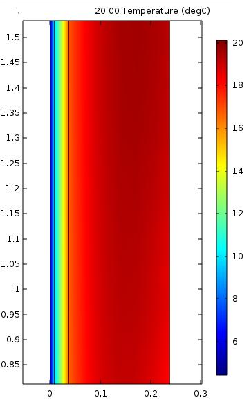
; 04:00 (b); 08:00 (c); 12:00 (d); 16:00 (e); 20:00 (f); 24:00 (g) 5.")
73 60 Figure 29: Demonstration of the passive heating and thermal storage function of the mass wall with the results from Study 2. Temperature field in mass wall at 00:00 (a); 04:00 (b); 08:00 (c); 12:00 (d); 16:00 (e); 20:00 (f); 24:00 (g) 5.4 Simulation Results (g) Two studies are carried out in order to modify the original model to adapt to Victoria s climate. Table 19 is a summary of all the parameters investigated and the optimized values for each parameter. Table 19.Summary of both parameters studies Original model Modified model Changed by Thickness of the mass wall L m 0.15m 0.2m 33% Thickness of the insulation wall L i 0.075m 0.1m 33% Emissivity of glass layer ε % Size of the interior vents H v 0.15m 0.22m 46% Thickness of the air channel L m 0.06m 50% Distance to the floor or ceiling H fl 0.085m 0.035m 59%
Transient Analysis of the Buoyancy Driven Flow in a Passive Solar System for Indoor Heating
 Excerpt from the Proceedings of the COMSOL Conference 2010 Paris Transient Analysis of the Buoyancy Driven Flow in a Passive Solar System for Indoor Heating Cammarata G., Petrone G. *, Cammarata L. Department
STUDY OF A PASSIVE SOLAR WINTER HEATING SYSTEM BASED ON TROMBE WALL
 STUDY OF A PASSIVE SOLAR WINTER HEATING SYSTEM BASED ON TROMBE WALL Dr. G.S.V.L.Narasimham Chief Research Scientist, RAC, Dept. of Mechanical Engineering, Indian Institute of Science,Bengaluru- 560012,
Experimental Performance and Numerical Simulation of Double Glass Wall Thana Ananacha
 Experimental Performance and Numerical Simulation of Double Glass Wall Thana Ananacha Abstract This paper reports the numerical and experimental performances of Double Glass Wall are investigated. Two
The energy performance of an airflow window
 The energy performance of an airflow window B.(Bram) Kersten / id.nr. 0667606 University of Technology Eindhoven, department of Architecture Building and Planning, unit Building Physics and Systems. 10-08-2011
Numerical study on thermal behavior of classical or composite Trombe solar walls
 Energy and Buildings 39 (007) 96 974 www.elsevier.com/locate/enbuild Numerical study on thermal behavior of classical or composite Trombe solar walls Jibao Shen a,b, Stéphane Lassue a, *, Laurent Zalewski
ELEC9712 High Voltage Systems. 1.2 Heat transfer from electrical equipment
 ELEC9712 High Voltage Systems 1.2 Heat transfer from electrical equipment The basic equation governing heat transfer in an item of electrical equipment is the following incremental balance equation, with
Towards a Quantitative Prediction of Ice Forming at the Surface of Airport Runways
 Towards a Quantitative Prediction of Ice Forming at the Surface of Airport Runways J. D. Wheeler 1, M. Rosa 2, L. Capobianco 2, P. Namy 1 1. SIMTEC, 8 rue Duployé, Grenoble, 38100, France 2. Groupe ADP
CAE 331/513 Building Science Fall 2016
 CAE 331/513 Building Science Fall 2016 Week 3: September 8, 2016 Heat transfer in buildings: Finish radiation, then solar radiation and windows Advancing energy, environmental, and sustainability research
Institut national des sciences appliquées de Strasbourg GENIE CLIMATIQUE ET ENERGETIQUE APPENDICES
 Institut national des sciences appliquées de Strasbourg GENIE CLIMATIQUE ET ENERGETIQUE APPENDICES DEVELOPMENT OF A TOOL, BASED ON THE THERMAL DYNAMIC SIMULATION SOFTWARE TRNSYS, WHICH RUNS PARAMETRIC
NUMERICAL MODELLING OF TEMPERATURE AND AIR FLOW DISTRIBUTION IN ENCLOSED ROOM
 NUMERICAL MODELLING OF TEMPERATURE AND AIR FLOW DISTRIBUTION IN ENCLOSED ROOM Igor Bonefacic 1, Bernard Frankovic 2, Ivan Vilicic 3, Vladimir Glazar 4 Faculty of Engineering, Vukovarska 58, Rijeka, Croatia,
Project 2. Introduction: 10/23/2016. Josh Rodriguez and Becca Behrens
 Project 2 Josh Rodriguez and Becca Behrens Introduction: Section I of the site Dry, hot Arizona climate Linen supply and cleaning facility Occupied 4am-10pm with two shifts of employees PHOENIX, ARIZONA
THERMAL PERFORMANCE EVALUATION OF AN INNOVATIVE DOUBLE GLAZING WINDOW
 THERMAL PERFORMANCE EVALUATION OF AN INNOVATIVE DOUBLE GLAZING WINDOW Luigi De Giorgi, Carlo Cima, Emilio Cafaro Dipartimento di Energetica, Politecnico di Torino, Torino, Italy Volfango Bertola School
C ONTENTS CHAPTER TWO HEAT CONDUCTION EQUATION 61 CHAPTER ONE BASICS OF HEAT TRANSFER 1 CHAPTER THREE STEADY HEAT CONDUCTION 127
 C ONTENTS Preface xviii Nomenclature xxvi CHAPTER ONE BASICS OF HEAT TRANSFER 1 1-1 Thermodynamics and Heat Transfer 2 Application Areas of Heat Transfer 3 Historical Background 3 1-2 Engineering Heat
Heat Transfer Convection
 Heat ransfer Convection Previous lectures conduction: heat transfer without fluid motion oday (textbook nearly 00 pages) Convection: heat transfer with fluid motion Research methods different Natural Convection
Computer Evaluation of Results by Room Thermal Stability Testing
 Computer Evaluation of Results by Room Thermal Stability Testing HANA CHARVÁTOVÁ 1, MARTIN ZÁLEŠÁK 1 Regional Research Centre CEBIA-Tech, Department of Automation and Control Engineering Faculty of Applied
Transient Heat Transfer Experiment. ME 331 Introduction to Heat Transfer. June 1 st, 2017
 Transient Heat Transfer Experiment ME 331 Introduction to Heat Transfer June 1 st, 2017 Abstract The lumped capacitance assumption for transient conduction was tested for three heated spheres; a gold plated
A Numerical Investigation on Active Chilled Beams for Indoor Air Conditioning
 Excerpt from the Proceedings of the COMSOL Conference 2008 Hannover A Numerical Investigation on Active Chilled Beams for Indoor Air Conditioning Cammarata G., Petrone G. * Department of Industrial and
Ceiling Radiant Cooling Panels Employing Heat-Conducting Rails: Deriving the Governing Heat Transfer Equations
 Authors may request permission to reprint or post on their personal or company Web site once the final version of the article has been published. A reprint permission form may be found at www.ashrae.org.
Patrick H. Oosthuizen and J.T. Paul Queen s University Kingston, ON, Canada
 Proceedings of the ASME 2012 International Mechanical Engineering Congress & Exposition IMECE2012 November 9-15, 2012, Houston, Texas, USA IMECE2012-87735 A NUMERICAL STUDY OF THE EFFECT OF AN IRRADIATED
Thermal mass vs. thermal response factors: determining optimal geometrical properties and envelope assemblies of building materials
 International Conference Passive and Low Energy Cooling 345 Thermal mass vs. thermal response factors: determining optimal geometrical properties and envelope assemblies of building materials K.J. Kontoleon
PERFORMANCE EVALUATION OF REFLECTIVE COATINGS ON ROOFTOP UNITS
 PERFORMANCE EVALUATION OF REFLECTIVE COATINGS ON ROOFTOP UNITS Report on DRAFT Prepared for: California Energy Commission 1516 9th Street Sacramento, CA 95814 Prepared by: Design & Engineering Services
Computational Modelling of the Impact of Solar Irradiance on Chemical Degradation of Painted Wall Hangings in an Historic Interior
 Computational Modelling of the Impact of Solar Irradiance on Chemical Degradation of Painted Wall Hangings in an Historic Interior Z. Huijbregts *1, A.W.M. van Schijndel 1, H.L. Schellen 1, K. Keune 2,
AR/IA 241 LN 231 Lecture 4: Fundamental of Energy
 Faculty of Architecture and Planning Thammasat University A/IA 24 LN 23 Lecture 4: Fundamental of Energy Author: Asst. Prof. Chalermwat Tantasavasdi. Heat For a specific substance, the heat given to the
A SIMPLE MODEL FOR THE DYNAMIC COMPUTATION OF BUILDING HEATING AND COOLING DEMAND. Kai Sirén AALTO UNIVERSITY
 A SIMPLE MODEL FOR THE DYNAMIC COMPUTATION OF BUILDING HEATING AND COOLING DEMAND Kai Sirén AALTO UNIVERSITY September 2016 CONTENT 1. FUNDAMENTALS OF DYNAMIC ENERGY CALCULATIONS... 3 1.1. Introduction...
If there is convective heat transfer from outer surface to fluid maintained at T W.
 Heat Transfer 1. What are the different modes of heat transfer? Explain with examples. 2. State Fourier s Law of heat conduction? Write some of their applications. 3. State the effect of variation of temperature
c. The Grashof number is the ratio of buoyant forces to viscous forces acting on a fluid.
 QUESTION 1. (0 pts) With respect to free convection: a. What is an extensive, quiescent fluid? (4 points) b. What are the two major physical considerations or forces for free convection? (4 points) c.
Department of Mechanical Engineering ME 96. Free and Forced Convection Experiment. Revised: 25 April Introduction
 CALIFORNIA INSTITUTE OF TECHNOLOGY Department of Mechanical Engineering ME 96 Free and Forced Convection Experiment Revised: 25 April 1994 1. Introduction The term forced convection refers to heat transport
PAUL RUDOLPH Oriental Masonic Gardens
 1 PAUL RUDOLPH Oriental Masonic Gardens Latitude _ 41.3 N Longitude _ 72.9 W Climate: transition between Cfa _ Humid Subtropical and Dfa_ Humid Continental climate 2 Paul Rudolph INTRODUCTION Fig. 1 -
Heat Transfer: Physical Origins and Rate Equations. Chapter One Sections 1.1 and 1.2
 Heat Transfer: Physical Origins and Rate Equations Chapter One Sections 1.1 and 1. Heat Transfer and Thermal Energy What is heat transfer? Heat transfer is thermal energy in transit due to a temperature
Greenhouse Steady State Energy Balance Model
 Greenhouse Steady State Energy Balance Model The energy balance for the greenhouse was obtained by applying energy conservation to the greenhouse system as a control volume and identifying the energy terms.
Chapter 5 MATHEMATICAL MODELING OF THE EVACATED SOLAR COLLECTOR. 5.1 Thermal Model of Solar Collector System
 Chapter 5 MATHEMATICAL MODELING OF THE EVACATED SOLAR COLLECTOR This chapter deals with analytical method of finding out the collector outlet working fluid temperature. A dynamic model of the solar collector
Experiment 1. Measurement of Thermal Conductivity of a Metal (Brass) Bar
 Bar") Experiment 1 Measurement of Thermal Conductivity of a Metal (Brass) Bar Introduction: Thermal conductivity is a measure of the ability of a substance to conduct heat, determined by the rate of heat flow
Experiment 1 Measurement of Thermal Conductivity of a Metal (Brass) Bar Introduction: Thermal conductivity is a measure of the ability of a substance to conduct heat, determined by the rate of heat flow
Documentation of the Solutions to the SFPE Heat Transfer Verification Cases
 Documentation of the Solutions to the SFPE Heat Transfer Verification Cases Prepared by a Task Group of the SFPE Standards Making Committee on Predicting the Thermal Performance of Fire Resistive Assemblies
PHYSICAL MECHANISM OF NATURAL CONVECTION
 1 NATURAL CONVECTION In this chapter, we consider natural convection, where any fluid motion occurs by natural means such as buoyancy. The fluid motion in forced convection is quite noticeable, since a
Analysis of the Cooling Design in Electrical Transformer
 Analysis of the Cooling Design in Electrical Transformer Joel de Almeida Mendes E-mail: joeldealmeidamendes@hotmail.com Abstract This work presents the application of a CFD code Fluent to simulate the
Computational Modeling of a Solar Thermoelectric Generator
 Computational Modeling of a Solar Thermoelectric Generator Undergraduate Thesis Presented in Partial Fulfillment of the Requirements for Graduation with Research Distinction at The Ohio State University
Energy flows and modelling approaches
 Energy flows and modelling approaches Energy flows in buildings external convection infiltration & ventilation diffuse solar external long-wave radiation to sky and ground local generation fabric heat
Summary of Dimensionless Numbers of Fluid Mechanics and Heat Transfer
 1. Nusselt number Summary of Dimensionless Numbers of Fluid Mechanics and Heat Transfer Average Nusselt number: convective heat transfer Nu L = conductive heat transfer = hl where L is the characteristic
INTERNATIONAL JOURNAL OF MECHANICAL ENGINEERING AND TECHNOLOGY (IJMET)
") INTERNATIONAL JOURNAL OF MECHANICAL ENGINEERING AND TECHNOLOGY (IJMET) International Journal of Mechanical Engineering and Technology (IJMET), ISSN 0976 ISSN 0976 6340 (Print) ISSN 0976 6359 (Online) Volume
INTERNATIONAL JOURNAL OF MECHANICAL ENGINEERING AND TECHNOLOGY (IJMET) International Journal of Mechanical Engineering and Technology (IJMET), ISSN 0976 ISSN 0976 6340 (Print) ISSN 0976 6359 (Online) Volume
TankExampleNov2016. Table of contents. Layout
 Table of contents Task... 2 Calculation of heat loss of storage tanks... 3 Properties ambient air Properties of air... 7 Heat transfer outside, roof Heat transfer in flow past a plane wall... 8 Properties
Department of Energy Science & Engineering, IIT Bombay, Mumbai, India. *Corresponding author: Tel: ,
 ICAER 2011 AN EXPERIMENTAL AND COMPUTATIONAL INVESTIGATION OF HEAT LOSSES FROM THE CAVITY RECEIVER USED IN LINEAR FRESNEL REFLECTOR SOLAR THERMAL SYSTEM Sudhansu S. Sahoo* a, Shinu M. Varghese b, Ashwin
ADVANCED ROOF COATINGS: MATERIALS AND THEIR APPLICATIONS
 ADVANCED ROOF COATINGS: MATERIALS AND THEIR APPLICATIONS Abstract J.M. Bell 1 and G.B. Smith 2 The use of low emittance and high solar reflectance coatings is widespread in window glazings, wall and roof
LAMINAR NATURAL CONVECTION IN VERTICAL 2D GLAZING CAVITIES
 Mechanical and Industrial Engineering University of Massachusetts, Amherst AMINAR NATURA CONVECTION IN VERTICA 2D GAZING CAVITIES Bhaskar Adusumalli ABSTRACT Finite element predictions of natural convection
Building heat system sizing
 May 6th, 203 MVK60 Heat and Mass Transfer Project report Building heat system sizing Arnaud BELTOISE Dept. of Energy Sciences, Faculty of Engineering, Lund University, Box 8, 2200 Lund, Sweden . Introduction
Computational analysis of the heat gain of buildings through their roofs using a heat transfer transient nonlinear model solved by numerical methods
 Computational analysis of the heat gain of buildings through their roofs using a heat transfer transient nonlinear model solved by numerical methods Carlos Armando De Castro Centro de Investigación en
EE-489 Modeling Project: Behavior of the. Temperature Changes in a Room
 EE-489 Modeling Project: Behavior of the 1 Temperature Changes in a Room Younes Sangsefidi, Saleh Ziaieinejad, Tarik Wahidi, and Takouda Pidename, Abstract A precise heat flow model, which predicts the
Solar Radiation Protections on Façades: A Case Study in a Hot Semi-Humid Climate
 Solar Radiation Protections on Façades: A Case Study in a Hot Semi-Humid Climate ADRIANA LIRA-OLIVER 1, JORGE ROJAS 2, GUADALUPE HUELSZ 2, GUILLERMO BARRIOS 2, FRANCISCO ROJAS 2 1 3S-Consulting for Sustainable
INSTRUCTOR: PM DR MAZLAN ABDUL WAHID
 SMJ 4463: HEAT TRANSFER INSTRUCTOR: PM ABDUL WAHID http://www.fkm.utm.my/~mazlan TEXT: Introduction to Heat Transfer by Incropera, DeWitt, Bergman, Lavine 5 th Edition, John Wiley and Sons Chapter 9 Natural
Introduction to Heat and Mass Transfer. Week 14
 Introduction to Heat and Mass Transfer Week 14 HW # 7 prob. 2 Hot water at 50C flows through a steel pipe (thermal conductivity 14 W/m-K) of 100 mm outside diameter and 8 mm wall thickness. During winter,
Chapter 1: 20, 23, 35, 41, 68, 71, 76, 77, 80, 85, 90, 101, 103 and 104.
 Chapter 1: 0, 3, 35, 1, 68, 71, 76, 77, 80, 85, 90, 101, 103 and 10. 1-0 The filament of a 150 W incandescent lamp is 5 cm long and has a diameter of 0.5 mm. The heat flux on the surface of the filament,
Chapter 7: Natural Convection
 7-1 Introduction 7- The Grashof Number 7-3 Natural Convection over Surfaces 7-4 Natural Convection Inside Enclosures 7-5 Similarity Solution 7-6 Integral Method 7-7 Combined Natural and Forced Convection
Chapter 9 NATURAL CONVECTION
 Heat and Mass Transfer: Fundamentals & Applications Fourth Edition in SI Units Yunus A. Cengel, Afshin J. Ghajar McGraw-Hill, 2011 Chapter 9 NATURAL CONVECTION PM Dr Mazlan Abdul Wahid Universiti Teknologi
Energy and Buildings
 Energy and Buildings 42 (2010) 1753 1758 Contents lists available at ScienceDirect Energy and Buildings journal homepage: www.elsevier.com/locate/enbuild A calculation method for the floor surface temperature
Heat Transfer Modeling using ANSYS FLUENT
 Lecture 1 - Introduction 14.5 Release Heat Transfer Modeling using ANSYS FLUENT 2013 ANSYS, Inc. March 28, 2013 1 Release 14.5 Outline Modes of Heat Transfer Basic Heat Transfer Phenomena Conduction Convection
CFD model to estimate the Effect of Tilt and Height on the Natural Air Flow inside a Solar Chimney
 7th WSEAS International Conference on Electric Power Systems, High Voltages, Electric Machines, Venice, Italy, November 21-23, 2007 53 CFD model to estimate the Effect of Tilt and Height on the Natural
Design strategy for Low e windows with effective insulation
 Design strategy for Low e windows with effective insulation Michael P.C. Watts, Impattern Solutions, www.impattern.com Keywords; insulating windows. low emission glass, ABSTRACT Optimal window glass assemblies
Theoretical Analysis of Overall Heat Loss Coefficient in a Flat Plate Solar Collector with an In-Built Energy Storage Using a Phase Change Material
 Theoretical Analysis of Overall Heat Loss Coefficient in a Flat Plate Solar Collector with an In-Built Energy Storage Using a Phase Change Material R. Sivakumar and V. Sivaramakrishnan Abstract Flat Plate
Thermal Systems Design MARYLAND. Fundamentals of heat transfer Radiative equilibrium Surface properties Non-ideal effects
 Thermal Systems Design Fundamentals of heat transfer Radiative equilibrium Surface properties Non-ideal effects Internal power generation Environmental temperatures Conduction Thermal system components
PERFORMANCE ANALYSIS OF A SINGLE BASIN DOUBLE SLOPE PASSIVE SOLAR STILL
 (IJAER) 212, Vol. No. 3, Issue No. II, February ISSN: 2231-5152 PERFORMANCE ANALYSIS OF A SINGLE BASIN DOUBLE SLOPE PASSIVE SOLAR STILL Vidya Sagar Gupta ABSTRACT An experimental study has been carried
Solar Flat Plate Thermal Collector
 Solar Flat Plate Thermal Collector INTRODUCTION: Solar heater is one of the simplest and basic technologies in the solar energy field. Collector is the heart of any solar heating system. It absorbs and
FORMULA SHEET. General formulas:
 FORMULA SHEET You may use this formula sheet during the Advanced Transport Phenomena course and it should contain all formulas you need during this course. Note that the weeks are numbered from 1.1 to
Natural Convection from a Long Horizontal Cylinder
 Natural Convection from a Long Horizontal Cylinder Hussein Awad Kurdi Saad Engineering Technical College of Al Najaf, Al-Furat Al-Awsat Technical University, Iraq ABSTRACT: Natural convection from a Long
Double-Skin Facade in Low-Latitude: Study on the Absorptance, Reflectance, and Transmittance of Direct Solar Radiation
 ouble-skin Facade in Low-Latitude: Study on the Absorptance, Reflectance, and Transmittance of irect Solar Radiation G-LO 011 Rosady Mulyadi epartment of Architecture Faculty of Engineering Hasanuddin
Natural convection heat transfer around a horizontal circular cylinder near an isothermal vertical wall
 Natural convection heat transfer around a horizontal circular cylinder near an isothermal vertical wall Marcel Novomestský 1, Richard Lenhard 1, and Ján Siažik 1 1 University of Žilina, Faculty of Mechanical
Improved energy management method for auxiliary electrical energy saving in a passive-solar-heated residence
 Energy and Buildings 34 (2002) 699 703 Improved energy management method for auxiliary electrical energy saving in a passive-solar-heated residence G.C. Bakos Department of Electrical Engineering and Electronics,
Effect of Periodic Variation of Sol-air Temperature on the Performance of Integrated Solar Collector Storage System
 Engineering, 2010, 2, 832-840 doi:10.4236/eng.2010.210106 Published Online October 2010 (http://www.scirp.org/journal/eng) Effect of Periodic Variation of Sol-air Temperature on the Performance of Integrated
Overview of Convection Heat Transfer
 Overview of Convection Heat Transfer Lecture Notes for ME 448/548 Gerald Recktenwald March 16, 2006 1 Introduction CFD is a powerful tool for engineering design involving fluid flow and heat transfer.
3.0 FINITE ELEMENT MODEL
 3.0 FINITE ELEMENT MODEL In Chapter 2, the development of the analytical model established the need to quantify the effect of the thermal exchange with the dome in terms of a single parameter, T d. In
Experimental Analysis for Natural Convection Heat Transfer through Vertical Cylinder
 Experimental Analysis for Natural Convection Heat Transfer through Vertical Cylinder 1 Shyam S. Kanwar, 2 Manoj K. Yadav, Saurabh Sharma 3 1,2,3 Assistant Professor 1 Department of Mechanical Engg. 1 Institute
True/False. Circle the correct answer. (1pt each, 7pts total) 3. Radiation doesn t occur in materials that are transparent such as gases.
 3. Radiation doesn t occur in materials that are transparent such as gases.") ME 323 Sample Final Exam. 120pts total True/False. Circle the correct answer. (1pt each, 7pts total) 1. A solid angle of 2π steradians defines a hemispherical shell. T F 2. The Earth irradiates the Sun.
ME 323 Sample Final Exam. 120pts total True/False. Circle the correct answer. (1pt each, 7pts total) 1. A solid angle of 2π steradians defines a hemispherical shell. T F 2. The Earth irradiates the Sun.
Development and Validation of Flat-Plate Collector Testing Procedures
 Development and Validation of Flat-Plate Collector Testing Procedures Report for February, 2007 Focus on Energy (FOE) supports solar thermal systems that displace conventional fuels by offering cash-back
Natural convective heat transfer in trapezoidal enclosure of box-type solar cooker
 Natural convective heat transfer in trapezoidal enclosure of box-type solar cooker Subodh Kumar * Centre for Energy Studies, Indian Institute of Technology, Hauz Khas, New Delhi 110016, India Received
Iterative calculation of the heat transfer coefficient
 Iterative calculation of the heat transfer coefficient D.Roncati Progettazione Ottica Roncati, Ferrara - Italy Aim The plate temperature of a cooling heat sink is an important parameter that has to be
Examination Heat Transfer
 Examination Heat Transfer code: 4B680 date: 17 january 2006 time: 14.00-17.00 hours NOTE: There are 4 questions in total. The first one consists of independent sub-questions. If necessary, guide numbers
BSE Public CPD Lecture Numerical Simulation of Thermal Comfort and Contaminant Transport in Rooms with UFAD system on 26 March 2010
 BSE Public CPD Lecture Numerical Simulation of Thermal Comfort and Contaminant Transport in Rooms with UFAD system on 26 March 2010 Organized by the Department of Building Services Engineering, a public
Study of air curtains used to restrict infiltration into refrigerated rooms
 Study of air curtains used to restrict infiltration into refrigerated rooms Gregory Verhaeghe 1, Marnix Van Belleghem 1, Arnout Willockx 1, Ivan Verhaert 1, Michel De Paepe 1 1 Ghent University, Department
Simulation of the Temperature Profile During Welding with COMSOL Multiphysics Software Using Rosenthal s Approach
 Simulation of the Temperature Profile During Welding with COMSOL Multiphysics Software Using Rosenthal s Approach A. Lecoanet*, D. G. Ivey, H. Henein Department of Chemical & Materials Engineering, University
FREE CONVECTIVE HEAT TRANSFER FROM AN OBJECT AT LOW RAYLEIGH NUMBER
 Free Convective Heat Transfer From an Object at Low Rayleigh Number FREE CONVECTIVE HEAT TRANSFER FROM AN OBJECT AT LOW RAYLEIGH NUMBER Md. Golam Kader and Khandkar Aftab Hossain * Department of Mechanical
5th WSEAS Int. Conf. on Heat and Mass transfer (HMT'08), Acapulco, Mexico, January 25-27, 2008
, Acapulco, Mexico, January 25-27, 2008") Numerical Determination of Temperature and Velocity Profiles for Forced and Mixed Convection Flow through Narrow Vertical Rectangular Channels ABDALLA S. HANAFI Mechanical power department Cairo university
Numerical Determination of Temperature and Velocity Profiles for Forced and Mixed Convection Flow through Narrow Vertical Rectangular Channels ABDALLA S. HANAFI Mechanical power department Cairo university
TREES Training for Renovated Energy Efficient Social housing
 TREES Training for Renovated Energy Efficient Social housing Intelligent Energy -Europe programme, contract n EIE/05/110/SI2.420021 Section 2 Tools 2.1 Simplified heating load calculation Tamas CSOKNYAI
Thermal Systems. What and How? Physical Mechanisms and Rate Equations Conservation of Energy Requirement Control Volume Surface Energy Balance
 Introduction to Heat Transfer What and How? Physical Mechanisms and Rate Equations Conservation of Energy Requirement Control Volume Surface Energy Balance Thermal Resistance Thermal Capacitance Thermal
NUMERICAL STUDY OF HEAT TRANSFER IN A FLAT PLAT THERMAL SOLAR COLLECTOR WITH PARTITIONS ATTACHED TO ITS GLAZING. Adel LAARABA.
 NUMERICAL STUDY OF HEAT TRANSFER IN A FLAT PLAT THERMAL SOLAR COLLECTOR WITH PARTITIONS ATTACHED TO ITS GLAZING Adel LAARABA. Department of physics. University of BATNA. (05000) Batna, Algeria Ccorresponding
Natural Ventilation. CFD modelling of a double-skin facade. Huw Birch. Supervisor: Abigail Hathway
 Natural Ventilation CFD modelling of a double-skin facade Huw Birch Supervisor: Abigail Hathway Introduction Given the high energy demands of traditional mechanical ventilation systems such as humidifiers,
Transport processes. 7. Semester Chemical Engineering Civil Engineering
 Transport processes 7. Semester Chemical Engineering Civil Engineering 1. Elementary Fluid Dynamics 2. Fluid Kinematics 3. Finite Control Volume Analysis 4. Differential Analysis of Fluid Flow 5. Viscous
THE INFLUENCE OF INCLINATION ANGLE ON NATURAL CONVECTION IN A RECTANGULAR ENCLOSURE
 THE INFLUENCE OF INCLINATION ANGLE ON NATURAL CONVECTION IN A RECTANGULAR ENCLOSURE Thamer Khalif Salem Mechanical Engineering, College of Engineering, Tikrit University, IRAQ. thamer_khalif@yahoo.com
Extensions to the Finite Element Technique for the Magneto-Thermal Analysis of Aged Oil Cooled-Insulated Power Transformers
 Journal of Electromagnetic Analysis and Applications, 2012, 4, 167-176 http://dx.doi.org/10.4236/jemaa.2012.44022 Published Online April 2012 (http://www.scirp.org/journal/jemaa) 167 Extensions to the
Design and Development of Solar Chimney
 Design and Development of Solar Chimney Ishan Upadhyay 1, Honey Kumar G. Vishwakarma 2, Dr. A. G. Bhave 3 1 Student, M.E Energy Engineering, K. J. Somaiya College of Engineering, Vidyavihar, Mumbai - 400077,
Heat Transfer and Natural Ventilation Airflow Rates from Single-sided Heated Solar Chimney for Buildings
 Heat Transfer and Natural Ventilation Airflow Rates from Single-sided Heated Solar Chimney for Buildings Angui Li* 1, Phillip Jones 2, Pingge Zhao 3 and Liping Wang 3 1 Professor, Department of Environmental
Natural Convection Heat Loss from A Partly Open Cubic Enclosure Timothy N Anderson 1,a * and Stuart E Norris 2,b
 Natural Convection Heat Loss from A Partly Open Cubic Enclosure Timothy N Anderson 1,a * and Stuart E Norris 2,b 1 Auckland University of Technology, New Zealand 2 University of Auckland, New Zealand a
MYcsvtu Notes HEAT TRANSFER BY CONVECTION
 www.mycsvtunotes.in HEAT TRANSFER BY CONVECTION CONDUCTION Mechanism of heat transfer through a solid or fluid in the absence any fluid motion. CONVECTION Mechanism of heat transfer through a fluid in
DYNAMIC INSULATION APPLIED TO THE RESIDENTIAL BUILDING (PART 2) Numerical Evaluation of Thermal Insulation Effect on Air Supply Window System
 Numerical Evaluation of Thermal Insulation Effect on Air Supply Window System") 3 5 7 8 9 DYNAMIC INSULATION APPLIED TO THE RESIDENTIAL BUILDING (PART ) Numerical Evaluation of Thermal Insulation Effect on Air Supply Window System ABSTRACT Sihwan Lee, Tanaka Miho, Shinsuke Kato 3
3 5 7 8 9 DYNAMIC INSULATION APPLIED TO THE RESIDENTIAL BUILDING (PART ) Numerical Evaluation of Thermal Insulation Effect on Air Supply Window System ABSTRACT Sihwan Lee, Tanaka Miho, Shinsuke Kato 3
Thermodynamics I Spring 1432/1433H (2011/2012H) Saturday, Wednesday 8:00am - 10:00am & Monday 8:00am - 9:00am MEP 261 Class ZA
 Saturday, Wednesday 8:00am - 10:00am & Monday 8:00am - 9:00am MEP 261 Class ZA") Thermodynamics I Spring 1432/1433H (2011/2012H) Saturday, Wednesday 8:00am - 10:00am & Monday 8:00am - 9:00am MEP 261 Class ZA Dr. Walid A. Aissa Associate Professor, Mech. Engg. Dept. Faculty of Engineering
Thermodynamics I Spring 1432/1433H (2011/2012H) Saturday, Wednesday 8:00am - 10:00am & Monday 8:00am - 9:00am MEP 261 Class ZA Dr. Walid A. Aissa Associate Professor, Mech. Engg. Dept. Faculty of Engineering
Mechanical Engineering. Postal Correspondence Course HEAT TRANSFER. GATE, IES & PSUs
 Heat Transfer-ME GATE, IES, PSU 1 SAMPLE STUDY MATERIAL Mechanical Engineering ME Postal Correspondence Course HEAT TRANSFER GATE, IES & PSUs Heat Transfer-ME GATE, IES, PSU 2 C O N T E N T 1. INTRODUCTION
COVENANT UNIVERSITY NIGERIA TUTORIAL KIT OMEGA SEMESTER PROGRAMME: MECHANICAL ENGINEERING
 COVENANT UNIVERSITY NIGERIA TUTORIAL KIT OMEGA SEMESTER PROGRAMME: MECHANICAL ENGINEERING COURSE: MCE 524 DISCLAIMER The contents of this document are intended for practice and leaning purposes at the
Heat Transfer. Energy from the Sun. Introduction
 Heat Transfer Energy from the Sun Introduction The sun rises in the east and sets in the west, but its exact path changes over the course of the year, which causes the seasons. In order to use the sun
Vertical Mantle Heat Exchangers for Solar Water Heaters
 for Solar Water Heaters Y.C., G.L. Morrison and M. Behnia School of Mechanical and Manufacturing Engineering The University of New South Wales Sydney 2052 AUSTRALIA E-mail: yens@student.unsw.edu.au Abstract
Arctice Engineering Module 3a Page 1 of 32
 Welcome back to the second part of the second learning module for Fundamentals of Arctic Engineering online. We re going to review in this module the fundamental principles of heat transfer. Exchange of
Dynamic thermal simulation of a solar chimney with PV modules
 International Conerence Passive and Low Energy Cooling 89 Dynamic thermal simulation o a solar chimney with PV modules J. Martí-Herrero and M.R. Heras-Celemin Energetic Eiciency in Building, CIEMAT, Madrid,
Numerical Investigation of Convective Heat Transfer in Pin Fin Type Heat Sink used for Led Application by using CFD
 GRD Journals- Global Research and Development Journal for Engineering Volume 1 Issue 8 July 2016 ISSN: 2455-5703 Numerical Investigation of Convective Heat Transfer in Pin Fin Type Heat Sink used for Led
Entropy 2011, 13, ; doi: /e OPEN ACCESS. Entropy Generation at Natural Convection in an Inclined Rectangular Cavity
 Entropy 011, 13, 100-1033; doi:10.3390/e1305100 OPEN ACCESS entropy ISSN 1099-4300 www.mdpi.com/journal/entropy Article Entropy Generation at Natural Convection in an Inclined Rectangular Cavity Mounir