Lecture 5: GMM Acoustic Modeling and Feature Extraction

Transcription

1 CS 224S / LINGUIST 285 Spoken Language Processing Andrew Maas Stanford University Spring 2017 Lecture 5: GMM Acoustic Modeling and Feature Extraction Original slides by Dan Jurafsky

2 Outline for Today Acoustic Model Acoustic likelihood for each state using Gaussians and Mixtures of Gaussians Where a state is progressively: CI Subphone (3ish per phone) Context Dependent (CD) phone (=triphones) State-tying of CD phone MFCC feature extraction Handling variation MLLR adaptation MAP adaptation (On your own)

3 Vector quantization: Discrete observations feature value 2 for state j feature value 1 for state j Slide from John-Paul Hosum

4 VQ We ll define a Codebook, which lists for each symbol A prototype vector, or codeword If we had 256 classes ( 8-bit VQ ), A codebook with 256 prototype vectors Given an incoming feature vector, we compare it to each of the 256 prototype vectors We pick whichever one is closest (by some distance metric) And replace the input vector by the index of this prototype vector

5 Vector Quantization Create a training set of feature vectors Cluster them into a small number of classes Represent each class by a discrete symbol For each class v k, we can compute the probability that it is generated by a given HMM state using Baum-Welch

6 Vector quantization: Discrete observations feature value 2 for state j feature value 1 for state j b j (v k ) = number of vectors with codebook index k in state j number of vectors in state j 14 1 = = 56 4 Slide from John-Paul Hosum

7 Directly Modeling Continuous Observations Gaussians Univariate Gaussians Baum-Welch for univariate Gaussians Multivariate Gaussians Baum-Welch for multivariate Gausians Gaussian Mixture Models (GMMs) Baum-Welch for GMMs

8 Better than VQ VQ is insufficient for real ASR Instead: Assume the possible values of the observation feature vector o t are normally distributed. Represent the observation likelihood function b j (o t ) as a Gaussian with mean µ j and variance s j 2 f (x µ,σ) = 1 σ 2π exp( (x µ)2 2σ 2 )

9 Gaussians are parameterized by mean and variance

10 Gaussians for Acoustic Modeling P(o q): A Gaussian parameterized by mean and variance: Different means P(o q) is highest here at mean P(o q) P(o q) low here, far from mean o

11 Using a (univariate) Gaussian as an acoustic likelihood estimator Let s suppose our observation was a single real-valued feature (instead of 39D vector) Then if we had learned a Gaussian over the distribution of values of this feature We could compute the likelihood of any given observation o t as follows:

12 Training a Univariate Gaussian A (single) Gaussian is characterized by a mean and a variance Imagine that we had some training data in which each state was labeled We could just compute the mean and variance from the data: µ i = 1 T T o t s.t. o t is state i t=1 σ i 2 = 1 T T (o t µ i ) 2 s.t. q t is state i t=1

13 Training Univariate Gaussians But we don t know which observation was produced by which state! What we want: to assign each observation vector o t to every possible state i, prorated by the probability the the HMM was in state i at time t. The probability of being in state i at time t is γ t (i)!! µ i = T t=1 T t=1 γ t (i)o t γ t (i) σ 2 i = T t=1 γ t (i)(o t µ i ) 2 T t=1 γ t (i)

14 Multivariate Gaussians Instead of a single mean µ and variance s: f (x µ,σ) = 1 σ 2π exp( (x µ)2 2σ 2 ) Vector of observations x modeled by vector of means µ and covariance matrix S f (x µ,σ) = 1 (2π) D / 2 Σ exp % 1 1/ 2 2 (x ( ' µ)t Σ 1 (x µ) * & )

15 Multivariate Gaussians Defining µ and S µ = E(x) [ ] Σ = E (x µ)(x µ) T So the i-jth element of S is: [ ] σ ij 2 = E (x i µ i )(x j µ j )

16 Gaussian Intuitions: Size of S µ = [0 0] µ = [0 0] µ = [0 0] S = I S = 0.6I S = 2I As S becomes larger, Gaussian becomes more spread out; as S becomes smaller, Gaussian more compressed From Andrew Ng s lecture notes for CS229

17 From Chen, Picheny et al lecture slides

18 [1 0] [.6 0] [0 1] [ 0 2] Different variances in different dimensions

19 Gaussian Intuitions: Off-diagonal As we increase the off-diagonal entries, more correlation between value of x and value of y Text and figures from Andrew Ng s lecture notes for CS229

20 Gaussian Intuitions: off-diagonal As we increase the off-diagonal entries, more correlation between value of x and value of y Text and figures from Andrew Ng s lecture notes for CS229

21 Gaussian Intuitions: off-diagonal and diagonal Decreasing non-diagonal entries (#1-2) Increasing variance of one dimension in diagonal (#3) Text and figures from Andrew Ng s lecture notes for CS229

22 In two dimensions From Chen, Picheny et al lecture slides

23 But: assume diagonal covariance I.e., assume that the features in the feature vector are uncorrelated This isn t true for FFT features, but is true for MFCC features, as we will see later. Computation and storage much cheaper if diagonal covariance. I.e. only diagonal entries are non-zero Diagonal contains the variance of each dimension s ii 2 So this means we consider the variance of each acoustic feature (dimension) separately

24 But we re not there yet Single Gaussian may do a bad job of modeling distribution in any dimension: Solution: Mixtures of Gaussians Figure from Chen, Picheney et al slides

25 Mixture of Gaussians to model a function %&* %&) %&( %&' %&! %&" %&# %&$ %!!!"!#!$ % $ # "!

26 GMMs Summary: each state has a likelihood function parameterized by: M Mixture weights M Mean Vectors of dimensionality D Either M Covariance Matrices of DxD Or more likely M Diagonal Covariance Matrices of DxD which is equivalent to M Variance Vectors of dimensionality D

27 Embedded Training

28 Initialization: Flat start Transition probabilities: set to zero any that you want to be structurally zero Set the rest to identical values Likelihoods: initialize µ and s of each state to global mean and variance of all training data

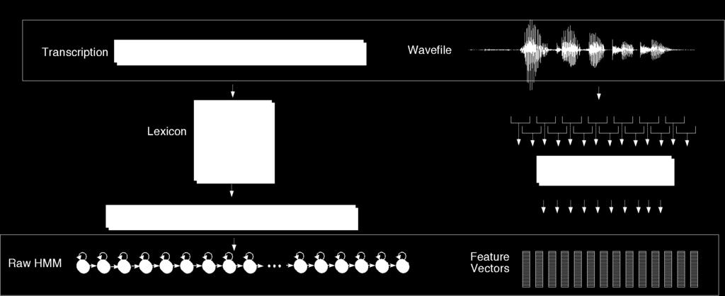
29 Embedded Training Given: phoneset, lexicon, transcribed wavefiles Build a whole sentence HMM for each sentence Initialize A probs to 0.5, or to zero Initialize B probs to global mean and variance Run multiple iterations of Baum Welch During each iteration, we compute forward and backward probabilities Use them to re-estimate A and B Run Baum-Welch until convergence.

30 Viterbi training Baum-Welch training says: We need to know what state we were in, to accumulate counts of a given output symbol o t We ll compute γ i (t), the probability of being in state i at time t, by using forward-backward to sum over all possible paths that might have been in state i and output o t. Viterbi training says: Instead of summing over all possible paths, just take the single most likely path Use the Viterbi algorithm to compute this Viterbi path Via forced alignment

31 Forced Alignment Computing the Viterbi path over the training data is called forced alignment Because we know which word string to assign to each observation sequence. We just don t know the state sequence. So we use a ij to constrain the path to go through the correct words And otherwise do normal Viterbi Result: state sequence!

32 Viterbi training equations Viterbi Baum-Welch a ˆ ij = n ij n i For all pairs of emitting states, 1 <= i, j <= N b ˆ (v ) = n j (s.t.o = v ) t k j k n j γ γ Where n ij is number of frames with transition from i to j in best path And n j is number of frames where state j is occupied

33 Outline for Today Acoustic Model Acoustic likelihood for each state using Gaussians and Mixtures of Gaussians Where a state is progressively: CI Subphone (3ish per phone) Context Dependent (CD) phone (=triphones) State-tying of CD phone MFCC feature extraction Handling variation MLLR adaptation MAP adaptation (On your own)

34 Phonetic context: different eh s w eh d y eh l b eh n

35 Modeling phonetic context The strongest factor affecting phonetic variability is the neighboring phone How to model that in HMMs? Idea: have phone models which are specific to context. Instead of Context-Independent (CI) phones We ll have Context-Dependent (CD) phones

36 CD phones: triphones Triphones Each triphone captures facts about preceding and following phone Monophone: p, t, k Triphone: iy-p+aa a-b+c means phone b, preceding by phone a, followed by phone c

37 Need with triphone models

38 Word-Boundary Modeling Word-Internal Context-Dependent Models OUR LIST : SIL AA+R AA-R L+IH L-IH+S IH-S+T S-T Cross-Word Context-Dependent Models OUR LIST : SIL-AA+R AA-R+L R-L+IH L-IH+S IH-S+T S-T+SIL Dealing with cross-words makes decoding harder!

39 Implications of Cross-Word Triphones Possible triphones: 50x50x50=125,000 How many triphone types actually occur? 20K word WSJ Task, numbers from Young et al Cross-word models: need 55,000 triphones But in training data only 18,500 triphones occur! Need to generalize models

40 Modeling phonetic context: some contexts look similar w iy r iy m iy n iy

41 Solution: State Tying Young, Odell, Woodland 1994 Decision-Tree based clustering of triphone states States which are clustered together will share their Gaussians We call this state tying, since these states are tied together to the same Gaussian.

42 Young et al state tying

43 State tying/clustering How do we decide which triphones to cluster together? Use phonetic features (or broad phonetic classes ) Stop Nasal Fricative Sibilant Vowel Lateral

44 Decision tree for clustering triphones for tying

45 Decision tree for clustering triphones for tying

46 State Tying: Young, Odell, Woodland ,-./01!&.23&3453&6. *!&')6.718**!1& 2396)*!" +:-.;)3&6.23&3453&6*.#3.#0!453&6* #$!"%& #$!"%&' ($!"%) *$!"%) <<<. +>-.;)8*#60.1&9.#!6. #0!453&6* #$!"%& #$!"%&' ($!"%) *$!"%) <<<. 7BB* #$!"%& #$!"%&' ($!"%) *$!"%) <<<.

47 Summary: Acoustic Modeling for LVCSR Increasingly sophisticated models For each state: Gaussians Multivariate Gaussians Mixtures of Multivariate Gaussians Where a state is progressively: CI Phone CI Subphone (3ish per phone) CD phone (=triphones) State-tying of CD phone Neural network acoustic models after all of the above Viterbi training

48 Summary: ASR Architecture Five easy pieces: ASR Noisy Channel architecture Feature Extraction: 39 MFCC features Acoustic Model: Gaussians for computing p(o q) Lexicon/Pronunciation Model HMM: what phones can follow each other Language Model N-grams for computing p(wi wi-1) Decoder Viterbi algorithm: dynamic programming for combining all these to get word sequence from speech! 64

49 Outline for Today Acoustic Model Acoustic likelihood for each state using Gaussians and Mixtures of Gaussians Where a state is progressively: CI Subphone (3ish per phone) Context Dependent (CD) phone (=triphones) State-tying of CD phone MFCC feature extraction Handling variation MLLR adaptation MAP adaptation (On your own)

50 Discrete Representation of Signal Represent continuous signal into discrete form. Image from Bryan Pellom

51 Sampling Original signal in red: If measure at green dots, will see a lower frequency wave and miss the correct higher frequency one!

52 WAV format Many formats, trade-offs in compression, quality Nice sound manipulation tool: Sox convert speech formats

53 MFCC Mel-Frequency Cepstral Coefficient (MFCC) Most widely used spectral representation in ASR

54 MFCC Mel-Frequency Cepstral Coefficient (MFCC) Most widely used spectral representation in ASR

55 Windowing Image from Bryan Pellom

56 MFCC

57 Discrete Fourier Transform computing a spectrum A 25 ms Hamming-windowed signal from [iy] And its spectrum as computed by DFT (plus other smoothing) Time (s) Sound pressure level (db/hz) Frequency (Hz)

58 MFCC

59 Mel-scale Human hearing is not equally sensitive to all frequency bands Less sensitive at higher frequencies, roughly > 1000 Hz I.e. human perception of frequency is non-linear:

60 Mel Filter Bank Processing Mel Filter bank Roughly uniformly spaced before 1 khz logarithmic scale after 1 khz

61 Mel-filter Bank Processing Apply the bank of Mel-scaled filters to the spectrum Each filter output is the sum of its filtered spectral components

62 MFCC

63 Log energy computation Compute the logarithm of the square magnitude of the output of Mel-filter bank

64 MFCC

65 The Cepstrum One way to think about this Separating the source and filter Speech waveform is created by A glottal source waveform Passes through a vocal tract which because of its shape has a particular filtering characteristic Remember articulatory facts from lecture 2: The vocal cord vibrations create harmonics The mouth is an amplifier Depending on shape of oral cavity, some harmonics are amplified more than others

66 George Miller figure

67 We care about the filter not the source Most characteristics of the source F0 Details of glottal pulse Don t matter for phone detection What we care about is the filter The exact position of the articulators in the oral tract So we want a way to separate these And use only the filter function

68 The Cepstrum The spectrum of the log of the spectrum Spectrum Log spectrum Spectrum of log spectrum

69 Another advantage of the Cepstrum DCT produces highly uncorrelated features If we use only the diagonal covariance matrix for our Gaussian mixture models, we can only handle uncorrelated features. In general we ll just use the first 12 cepstral coefficients (we don t want the later ones which have e.g. the F0 spike)

70 MFCC

71 Delta features Speech signal is not constant slope of formants, change from stop burst to release So in addition to the cepstral features Need to model changes in the cepstral features over time. delta features double delta (acceleration) features

72 Delta and double-delta Derivative: in order to obtain temporal information

73 Typical MFCC features Window size: 25ms Window shift: 10ms Pre-emphasis coefficient: 0.97 MFCC: 12 MFCC (mel frequency cepstral coefficients) 1 energy feature 12 delta MFCC features 12 double-delta MFCC features 1 delta energy feature 1 double-delta energy feature Total 39-dimensional features

74 Why is MFCC so popular? Efficient to compute Incorporates a perceptual Mel frequency scale Separates the source and filter IDFT(DCT) decorrelates the features Necessary for diagonal assumption in HMM modeling There are alternatives like PLP Choice matters less for neural network acoustic models (in future lectures)

75 Outline for Today Acoustic Model Acoustic likelihood for each state using Gaussians and Mixtures of Gaussians Where a state is progressively: CI Subphone (3ish per phone) CD phone (=triphones) State-tying of CD phone MFCC feature extraction Handling variation MLLR adaptation MAP adaptation (On your own)

76 Acoustic Model Adaptation Shift the means and variances of Gaussians to better match the input feature distribution Maximum Likelihood Linear Regression (MLLR) Maximum A Posteriori (MAP) Adaptation For both speaker adaptation and environment adaptation Widely used!

77 Maximum Likelihood Linear Regression (MLLR) Leggetter, C.J. and P. Woodland Maximum likelihood linear regression for speaker adaptation of continuous density hidden Markov models. Computer Speech and Language 9:2, Given: a trained AM a small adaptation dataset from a new speaker Learn new values for the Gaussian mean vectors Not by just training on the new data (too small) But by learning a linear transform which moves the means.

78 Maximum Likelihood Linear Regression (MLLR) Estimates a linear transform matrix (W) and bias vector (w) to transform HMM model means: µ new = W r µ old + ω r Transform estimated to maximize the likelihood of the adaptation data Slide from Bryan Pellom

79 MLLR New equation for output likelihood b j (o t ) = 1 (2π) n / 2 Σ j exp & 1 1/ 2 2 (o ) ( t (Wµ j + ω)) Σ j 1 (o t (Wµ j + ω)) T + ' *

80 MLLR Q: Why is estimating a linear transform from adaptation data different than just training on the data? A: Even from a very small amount of data we can learn 1 single transform for all triphones! So small number of parameters. A2: If we have enough data, we could learn more transforms (but still less than the number of triphones). One per phone (~50) is often done.

81 MLLR: Learning Given a small labeled adaptation set (a couple sentences) a trained AM Do forward-backward alignment on adaptation set to compute state occupation probabilities γ j (t). W can now be computed by solving a system of simultaneous equations involving γ j (t)

82 MLLR performance on baby task (RM) (Leggetter and Woodland 1995) Only 3 sentences! 11 seconds of speech!

83 MLLR doesn t need supervised adaptation set!

84 Slide from Bryan Pellom

85 Slide from Bryan Pellom after Huang et al

86 Summary MLLR: works on small amounts of adaptation data MAP: Maximum A Posterior Adaptation Works well on large adaptation sets Acoustic adaptation techniques are quite successful at dealing with speaker variability If we can get 10 seconds with the speaker.