Introduction to Bayesian Inference: Supplemental Topics

Transcription

1 Introduction to Bayesian Inference: Supplemental Topics Tom Loredo Cornell Center for Astrophysics and Planetary Science CASt Summer School 7 8 June / 75

2 Supplemental Topics 1 Parametric bootstrapping vs. posterior sampling 2 Estimation and model comparison for binary outcomes 3 Basic inference with normal errors 4 Poisson distribution; the on/off problem 5 Assigning priors 2 / 75

3 Supplemental Topics 1 Parametric bootstrapping vs. posterior sampling 2 Estimation and model comparison for binary outcomes 3 Basic inference with normal errors 4 Poisson distribution; the on/off problem 5 Assigning priors 3 / 75

4 Likelihood-Based Parametric Bootstrapping Likelihood L(θ) p(d obs θ). Log-likelihood L(θ) = ln L(θ). For the Gaussian example, L(µ) = i i 1 [ σ 2π exp (x i µ) 2 ] 2σ 2 exp [ (x i µ) 2 ] 2σ 2 L(µ) = 1 (x i µ) 2 2 σ 2 + Const = χ2 (µ) 2 i + Const 4 / 75

5 Incorrect Parametric Bootstrapping P = (A, T ) A ˆP(D obs ) Histograms/contours of best-fit estimates from D p(d ˆθ(D obs )) provide poor confidence regions no better (possibly worse) than using a least-squares/χ 2 covariance matrix. What s wrong with the population of ˆθ points for this purpose? T 5 / 75

6 Incorrect Parametric Bootstrapping P = (A, T ) A ˆP(D obs ) Histograms/contours of best-fit estimates from D p(d ˆθ(D obs )) provide poor confidence regions no better (possibly worse) than using a least-squares/χ 2 covariance matrix. What s wrong with the population of ˆθ points for this purpose? T The estimates are skewed down and to the right, indicating the truth must be up and to the left. Do not mistake variability of the estimator with the uncertainty of the estimate! 5 / 75

7 Key idea: Use likelihood ratios to define confidence regions. I.e., use L or χ 2 differences to define regions. Estimate parameter values via maximum likelihood (min χ 2 ) L max. Pick a constant L. Then (D) = {θ : L(θ) > L max L} Coverage calculation: 1. Fix θ 0 = ˆθ(D obs ) (plug-in approx n) 2. Simulate a dataset from p(d θ 0 ) L D (θ) Find maximum likelihood estimate ˆθ(D) Calculate L = L D (ˆθ D ) L D (θ 0 ) 5. Goto (2) for N total iterations 6. Histogram the L values to find coverage vs. L (fraction of sim ns with smaller L) Report (D obs ) with L chosen for desired approximate CL. 6 / 75

8 A L Calibration A Reported Region T T The CL is approximate due to: Monte Carlo error in calibrating L The plug-in approximation 7 / 75

9 Credible Region Via Posterior Sampling Monte Carlo algorithm for finding credible regions: 1. Create a RNG that can sample θ from p(θ D obs ) 2. Draw N samples; record θ i and q i = π(θ i )L(µ i ) 3. Sort the samples by the q i values 4. An HPD region of probability P is the θ region spanned by the 100P% of samples with highest q i Note that no dataset other than D obs is ever considered. P is a property of the particular interval reported. A T 8 / 75

10 This complication is the rule rather than the exception! Simple example: Estimate the mean and standard deviation of a normal distribution (µ = 5, σ = 1, N = 5; 200 samples): 9 / 75

11 Supplemental Topics 1 Parametric bootstrapping vs. posterior sampling 2 Estimation and model comparison for binary outcomes 3 Basic inference with normal errors 4 Poisson distribution; the on/off problem 5 Assigning priors 10 / 75

12 Binary Outcomes: Parameter Estimation M = Existence of two outcomes, S and F ; for each case or trial, the probability for S is α; for F it is (1 α) H i = Statements about α, the probability for success on the next trial seek p(α D, M) D = Sequence of results from N observed trials: Likelihood: FFSSSSFSSSFS (n = 8 successes in N = 12 trials) p(d α, M) = p(failure α, M) p(failure α, M) = α n (1 α) N n = L(α) 11 / 75

13 Prior Starting with no information about α beyond its definition, use as an uninformative prior p(α M) = 1. Justifications: Intuition: Don t prefer any α interval to any other of same size Bayes s justification: Ignorance means that before doing the N trials, we have no preference for how many will be successes: P(n success M) = 1 N + 1 p(α M) = 1 Consider this a convention an assumption added to M to make the problem well posed. 12 / 75

14 Prior Predictive p(d M) = dα α n (1 α) N n = B(n + 1, N n + 1) = n!(n n)! (N + 1)! A Beta integral, B(a, b) dx x a 1 (1 x) b 1 = Γ(a)Γ(b) Γ(a+b). 13 / 75

15 Posterior p(α D, M) = (N + 1)! n!(n n)! αn (1 α) N n A Beta distribution. Summaries: Best-fit: ˆα = n n+1 N = 2/3; α = N Uncertainty: σ α = (n+1)(n n+1) 0.12 (N+2) 2 (N+3) Find credible regions numerically, or with incomplete beta function Note that the posterior depends on the data only through n, not the N binary numbers describing the sequence. n is a (minimal) sufficient statistic. 14 / 75

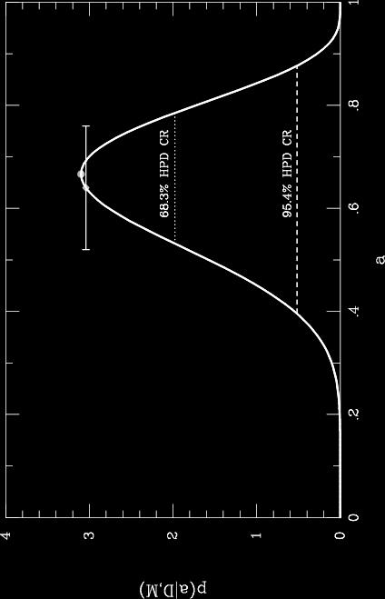
16 15 / 75

17 Binary Outcomes: Model Comparison Equal Probabilities? M 1 : α = 1/2 M 2 : α [0, 1] with flat prior. Maximum Likelihoods M 1 : p(d M 1 ) = 1 = N M 2 : L(ˆα) = ( ) 2 n ( ) 1 N n = p(d M 1 ) p(d ˆα, M 2 ) = 0.51 Maximum likelihoods favor M 2 (failures more probable). 16 / 75

18 Bayes Factor (ratio of model likelihoods) p(d M 1 ) = 1 2 N ; and p(d M n!(n n)! 2) = (N + 1)! B 12 p(d M 1) p(d M 2 ) (N + 1)! = n!(n n)!2 N = 1.57 Bayes factor (odds) favors M 1 (equiprobable). Note that for n = 6, B 12 = 2.93; for this small amount of data, we can never be very sure results are equiprobable. If n = 0, B 12 1/315; if n = 2, B 12 1/4.8; for extreme data, 12 flips can be enough to lead us to strongly suspect outcomes have different probabilities. (Frequentist significance tests can reject null for any sample size.) 17 / 75

19 Binary Outcomes: Binomial Distribution Suppose D = n (number of heads in N trials), rather than the actual sequence. What is p(α n, M)? Likelihood Let S = a sequence of flips with n heads. p(n α, M) = p(s α, M) p(n S, α, M) S α n (1 α) N n # successes = n = α n (1 α) N n C n,n C n,n = # of sequences of length N with n heads. p(n α, M) = N! n!(n n)! αn (1 α) N n The binomial distribution for n given α, N. 18 / 75

20 Posterior p(α n, M) = N! n!(n n)! αn (1 α) N n p(n M) p(n M) = = N! n!(n n)! 1 N + 1 dα α n (1 α) N n p(α n, M) = (N + 1)! n!(n n)! αn (1 α) N n Same result as when data specified the actual sequence. 19 / 75

21 Another Variation: Negative Binomial Suppose D = N, the number of trials it took to obtain a predifined number of successes, n = 8. What is p(α N, M)? Likelihood p(n α, M) is probability for n 1 successes in N 1 trials, times probability that the final trial is a success: p(n α, M) = = (N 1)! (n 1)!(N n)! αn 1 (1 α) N n α (N 1)! (n 1)!(N n)! αn (1 α) N n The negative binomial distribution for N given α, n. 20 / 75

22 Posterior p(α D, M) = C n,n α n (1 α) N n p(d M) p(d M) = C n,n dα α n (1 α) N n p(α D, M) = Same result as other cases. (N + 1)! n!(n n)! αn (1 α) N n 21 / 75

23 Final Variation: Meteorological Stopping Suppose D = (N, n), the number of samples and number of successes in an observing run whose total number was determined by the weather at the telescope. What is p(α D, M )? (M adds info about weather to M.) Likelihood p(d α, M ) is the binomial distribution times the probability that the weather allowed N samples, W (N): p(d α, M N! ) = W (N) n!(n n)! αn (1 α) N n Let C n,n = W (N) ( N n). We get the same result as before! 22 / 75

24 Likelihood Principle To define L(H i ) = p(d obs H i, I ), we must contemplate what other data we might have obtained. But the real sample space may be determined by many complicated, seemingly irrelevant factors; it may not be well-specified at all. Should this concern us? Likelihood principle: The result of inferences depends only on how p(d obs H i, I ) varies w.r.t. hypotheses. We can ignore aspects of the observing/sampling procedure that do not affect this dependence. This happens because no sums of probabilities for hypothetical data appear in Bayesian results; Bayesian calculations condition on D obs. This is a sensible property that frequentist methods do not share. Frequentist probabilities are long run rates of performance, and depend on details of the sample space that are irrelevant in a Bayesian calculation. 23 / 75

25 Goodness-of-fit Violates the Likelihood Principle Theory (H 0 ) The number of A stars in a cluster should be 0.1 of the total. Observations 5 A stars found out of 96 total stars observed. Theorist s analysis Calculate χ 2 using n A = 9.6 and n X = Significance level is p(> χ 2 H 0 ) = 0.12 (or 0.07 using more rigorous binomial tail area). Theory is accepted. 24 / 75

26 Observer s analysis Actual observing plan was to keep observing until 5 A stars seen! Random quantity is N tot, not n A ; it should follow the negative binomial dist n. Expect N tot = 50 ± 21. p(> χ 2 H 0 ) = Theory is rejected. Telescope technician s analysis A storm was coming in, so the observations would have ended whether 5 A stars had been seen or not. The proper ensemble should take into account p(storm)... Bayesian analysis The Bayes factor is the same for binomial or negative binomial likelihoods, and slightly favors H 0. Include p(storm) if you want it will drop out! 25 / 75

27 Probability & frequency Frequencies are relevant when modeling repeated trials, or repeated sampling from a population or ensemble. Frequencies are observables When available, can be used to infer probabilities for next trial When unavailable, can be predicted Bayesian/Frequentist relationships Relationships between probability and frequency Long-run performance of Bayesian procedures 26 / 75

28 Probability & frequency in IID settings Frequency from probability Bernoulli s law of large numbers: In repeated i.i.d. trials, given P(success...) = α, predict n success N total α as N total If p(x) does not change from sample to sample, it may be interpreted as a frequency distribution. Probability from frequency Bayes s An Essay Towards Solving a Problem in the Doctrine of Chances First use of Bayes s theorem: Probability for success in next trial of i.i.d. sequence: E(α) n success N total as N total If p(x) does not change from sample to sample, it may be estimated from a frequency distribution. 27 / 75

29 Supplemental Topics 1 Parametric bootstrapping vs. posterior sampling 2 Estimation and model comparison for binary outcomes 3 Basic inference with normal errors 4 Poisson distribution; the on/off problem 5 Assigning priors 28 / 75

30 Inference With Normals/Gaussians Gaussian PDF p(x µ, σ) = 1 σ (x µ) 2 2π e 2σ 2 over [, ] Common abbreviated notation: x N(µ, σ 2 ) Parameters µ = x dx x p(x µ, σ) σ 2 = (x µ) 2 dx (x µ) 2 p(x µ, σ) 29 / 75

31 Gauss s Observation: Sufficiency Suppose our data consist of N measurements, d i = µ + ɛ i. Suppose the noise contributions are independent, and ɛ i N (0, σ 2 ). p(d µ, σ, M) = i p(d i µ, σ, M) = p(ɛ i = d i µ µ, σ, M) i = 1 [ σ 2π exp (d i µ) 2 ] 2σ 2 i 1 = σ N e Q(µ)/2σ2 (2π) N/2 30 / 75

32 Find dependence of Q on µ by completing the square: Q = i (d i µ) 2 [Note: Q/σ 2 = χ 2 (µ)] = i ( = i d 2 i + i ) d 2 i = N(µ d) 2 + µ 2 2 i d i µ + Nµ 2 2Nµd where d 1 N ( i d 2 i ) Nd 2 = N(µ d) 2 + Nr 2 where r 2 1 (d i d) 2 N i i d i 31 / 75

33 Likelihood depends on {d i } only through d and r: L(µ, σ) = 1 σ N exp (2π) N/2 ( Nr 2 2σ 2 ) ) N(µ d)2 exp ( 2σ 2 The sample mean and variance are sufficient statistics. This is a miraculous compression of information the normal dist n is highly abnormal in this respect! 32 / 75

34 Estimating a Normal Mean Problem specification Model: d i = µ + ɛ i, ɛ i N(0, σ 2 ), σ is known I = (σ, M). Parameter space: µ; seek p(µ D, σ, M) Likelihood p(d µ, σ, M) = 1 σ N exp ( Nr 2 (2π) N/2 2σ 2 ) N(µ d)2 exp ( 2σ 2 ) exp ( ) N(µ d)2 2σ 2 33 / 75

35 Uninformative prior Translation invariance p(µ) C, a constant. This prior is improper unless bounded. Prior predictive/normalization p(d σ, M) = ) N(µ d)2 dµ C exp ( 2σ 2 = C(σ/ N) 2π... minus a tiny bit from tails, using a proper prior. 34 / 75

36 Posterior p(µ D, σ, M) = ) 1 ( (σ/ N) 2π exp N(µ d)2 2σ 2 Posterior is N(d, w 2 ), with standard deviation w = σ/ N. 68.3% HPD credible region for µ is d ± σ/ N. Note that C drops out limit of infinite prior range is well behaved. 35 / 75

37 Informative Conjugate Prior Posterior Use a normal prior, µ N(µ 0, w 2 0 ). Conjugate because the posterior turns out also to be normal. Normal N( µ, w 2 ), but mean, std. deviation shrink towards prior. Define B = w 2, so B < 1 and B = 0 when w w 2 +w0 2 0 is large. Then µ = d + B (µ 0 d) w = w 1 B Principle of stable estimation The prior affects estimates only when data are not informative relative to prior. 36 / 75

38 Conjugate normal examples: Data have d = 3, σ/ N = 1 Priors at µ 0 = 10, with w = {5, 2} Prior L Post ) 0.25 p(x 0.20 ) 0.25 p(x x x / 75

39 Estimating a Normal Mean: Unknown σ Problem specification Model: d i = µ + ɛ i, ɛ i N(0, σ 2 ), σ is unknown Parameter space: (µ, σ); seek p(µ D, M) Likelihood p(d µ, σ, M) = 1 σ N exp (2π) N/2 1 σ N e Q/2σ2 ( Nr 2 2σ 2 where Q = N [ r 2 + (µ d) 2] ) ) N(µ d)2 exp ( 2σ 2 38 / 75

40 Uninformative Priors Assume priors for µ and σ are independent. Translation invariance p(µ) C, a constant. Scale invariance p(σ) 1/σ (flat in log σ). Joint Posterior for µ, σ p(µ, σ D, M) 1 e Q(µ)/2σ2 σn+1 39 / 75

41 Marginal Posterior p(µ D, M) dσ 1 σ N+1 e Q/2σ2 Let τ = Q Q so σ = 2σ 2 2τ and dσ = τ 3/2 Q 2 dτ p(µ D, M) 2 N/2 Q N/2 dτ τ N 2 1 e τ Q N/2 40 / 75

42 Write Q = Nr 2 [1 + ( ) ] 2 µ d r and normalize: p(µ D, M) = ( N 2 1) [! 1 ( N 2 3 ) ( ) 2 ] N/2 µ d 2! π r N r/ N Student s t distribution, with t = (µ d) r/ N A bell curve, but with power-law tails Large N: p(µ D, M) e N(µ d)2 /2r 2 This is the rigorous way to adjust σ so χ 2 /dof = 1. It doesn t just plug in a best σ; it slightly broadens posterior to account for σ uncertainty. 41 / 75

43 Student t examples: 1 p(x) ( ) n+1 1+ x2 2 n Location = 0, scale = 1 Degrees of freedom = {1, 2, 3, 5, 10, } normal p(x) x 42 / 75

44 Gaussian Background Subtraction Measure background rate b = ˆb ± σ b with source off. Measure total rate r = ˆr ± σ r with source on. Infer signal source strength s, where r = s + b. With flat priors, [ ] (b ˆb) 2 p(s, b D, M) exp 2σ 2 b exp [ ] (s + b ˆr)2 2σr 2 43 / 75

45 Marginalize b to summarize the results for s (complete the square to isolate b dependence; then do a simple Gaussian integral over b): ] (s ŝ)2 p(s D, M) exp [ 2σs 2 ŝ = ˆr ˆb σ 2 s = σ 2 r + σ 2 b Background subtraction is a special case of background marginalization; i.e., marginalization told us to subtract a background estimate. Recall the standard derivation of background uncertainty via propagation of errors based on Taylor expansion (statistician s Delta-method). Marginalization provides a generalization of error propagation without approximation! 44 / 75

46 Supplemental Topics 1 Parametric bootstrapping vs. posterior sampling 2 Estimation and model comparison for binary outcomes 3 Basic inference with normal errors 4 Poisson distribution; the on/off problem 5 Assigning priors 45 / 75

47 Poisson Dist n: Infer a Rate from Counts Problem: Observe n counts in T ; infer rate, r Likelihood Prior L(r) p(n r, M) = p(n r, M) = (rt )n e rt n! Two simple standard choices (or conjugate gamma dist n): r known to be nonzero; it is a scale parameter: 1 1 p(r M) = ln(r u /r l ) r r may vanish; require p(n M) Const: p(r M) = 1 r u 46 / 75

48 Prior predictive Posterior p(n M) = 1 r u 1 n! = A gamma distribution: ru 0 rut dr(rt ) n e rt 1 1 r u T n! 0 1 r u T for r u n T d(rt )(rt ) n e rt p(r n, M) = T (rt )n e rt n! 47 / 75

49 Gamma Distributions A 2-parameter family of distributions over nonnegative x, with shape parameter α and scale parameter s: p Γ (x α, s) = 1 ( x ) α 1 e x/s sγ(α) s Moments: E(x) = sα Var(x) = s 2 α Our posterior corresponds to α = n + 1, s = 1/T. Mode ˆr = n n+1 T ; mean r = T (shift down 1 with 1/r prior) Std. dev n σ r = n+1 T ; credible regions found by integrating (can use incomplete gamma function) 48 / 75

50 Mode Mean T =2 s, n =10 p(r n,m) (s) r (s 1 ) 49 / 75

51 Conjugate prior Note that a gamma distribution prior is the conjugate prior for the Poisson sampling distribution: p(r n, M ) Gamma(r α, s) Pois(n rt ) r α 1 e r/s r n e rt r α+n 1 exp[ r(t + 1/s)] For α = 1, s, the gamma prior becomes an uninformative flat prior; posterior is proper even for n = 0 Useful conventions Use a flat prior for a rate that may be zero Use a log-flat prior ( 1/r) for a nonzero scale parameter Use proper (normalized, bounded) priors Plot posterior with abscissa that makes prior flat (use log r abscissa for scale parameter case) 50 / 75

52 Infer a Signal in a Known Background Problem: As before, but r = s + b with b known; infer s p(s n, b, M) = C T [(s + b)t ]n e (s+b)t n! C 1 = e bt d(st ) (s + b) n T n e st n! 0 n (bt ) i = e bt i! i=0 A sum of Poisson probabilities for background events; it can be evaluated using the incomplete gamma function. (Helene 1983) 51 / 75

53 Basic problem The On/Off Problem Look off-source; unknown background rate b Count N off photons in interval T off Look on-source; rate is r = s + b with unknown signal s Count N on photons in interval T on Infer s Conventional solution ˆb = N off /T off ; σ b = N off /T off ˆr = N on /T on ; σ r = N on /T on ŝ = ˆr ˆb; σ s = σr 2 + σb 2 But ŝ can be negative! 52 / 75

54 Bayesian Solution to On/Off Problem First consider off-source data; use it to estimate b: p(b N off, I off ) = T off(bt off ) N off e bt off N off! Use this as a prior for b to analyze on-source data. For on-source analysis I all = (I on, N off, I off ): p(s, b N on ) p(s)p(b)[(s + b)t on ] Non e (s+b)ton I all p(s I all ) is flat, but p(b I all ) = p(b N off, I off ), so p(s, b N on, I all ) (s + b) Non b N off e ston e b(ton+t off) 53 / 75

55 Now marginalize over b; p(s N on, I all ) = db p(s, b N on, I all ) db (s + b) Non b N off e ston e b(ton+t off) Expand (s + b) Non and do the resulting Γ integrals: p(s N on, I all ) = C i N on T on (st on ) i e ston C i i! i=0 ( 1 + T ) i off (N on + N off i)! T on (N on i)! Posterior is a weighted sum of Gamma distributions, each assigning a different number of on-source counts to the source. (Evaluate via recursive algorithm or confluent hypergeometric function.) 54 / 75

56 Example On/Off Posteriors Short Integrations T on = 1 55 / 75

57 Example On/Off Posteriors Long Background Integrations T on = 1 56 / 75

58 Second Solution of the On/Off Problem Consider all the data at once; the likelihood is a product of Poisson distributions for the on- and off-source counts: L(s, b) p(n on, N off s, b, I ) [(s + b)t on ] Non e (s+b)ton (bt off ) N off e bt off Take joint prior to be flat; find the joint posterior and marginalize over b; p(s N on, I on ) = db p(s, b I ) L(s, b) db (s + b) Non b N off e ston e b(ton+t off) same result as before. 57 / 75

59 Third Solution: Data Augmentation Suppose we knew the number of on-source counts that are from the background, N b. Then the on-source likelihood is simple: p(n on s, N b, I all ) = Pois(N on N b ; st on ) = (st on) Non N b (N on N b )! e ston Data augmentation: Pretend you have the missing data, then marginalize to account for its uncertainty: p(n on s, I all ) = N on N b =0 p(n b I all ) p(n on s, N b, I all ) = N b Predictive for N b Pois(N on N b ; st on ) p(n b I all ) = = db p(b N off, I off ) p(n b b, I on ) db Gamma(b) Pois(N b ; bt on ) same result as before. 58 / 75

60 A profound consistency We solved the on/off problem in multiple ways, always finding the same final results. This reflects something fundamental about Bayesian inference. R. T. Cox proposed two necessary conditions for a quantification of uncertainty: It should duplicate deductive logic when there is no uncertainty Different decompositions of arguments should produce the same final quantifications (internal consistency) Great surprise: These conditions are sufficient; they lead to the probability axioms. E. T. Jaynes and others refined and simplified Cox s analysis. 59 / 75

61 Multibin On/Off The more typical on/off scenario: Data = spectrum or image with counts in many bins Model M gives signal rate s k (θ) in bin k, parameters θ To infer θ, we need the likelihood: L(θ) = k p(n onk, N off k s k (θ), M) For each k, we have an on/off problem as before, only we just need the marginal likelihood for s k (not the posterior). The same C i coefficients arise. XSPEC and CIAO/Sherpa provide this as an option van Dyk + (2001) does the same thing via data augmentation (Monte Carlo) 60 / 75

62 Supplemental Topics 1 Parametric bootstrapping vs. posterior sampling 2 Estimation and model comparison for binary outcomes 3 Basic inference with normal errors 4 Poisson distribution; the on/off problem 5 Assigning priors 61 / 75

63 Well-Posed Problems The rules (BT, LTP,... ) express desired probabilities in terms of other probabilities To get a numerical value out, at some point we have to put numerical values in Direct probabilities are probabilities with numerical values determined directly by premises (via modeling assumptions, symmetry arguments, previous calculations, desperate presumption... ) An inference problem is well posed only if all the needed probabilities are assignable based on the context. We may need to add new assumptions as we see what needs to be assigned. We may not be entirely comfortable with what we need to assume! (Remember Euclid s fifth postulate!) Should explore how results depend on uncomfortable assumptions ( robustness ) 62 / 75

64 Contextual/prior/background information Bayes s theorem moves the data and hypothesis propositions wrt the solidus: P(H i D obs, I ) = P(H i I ) P(D obs H i, I ) P(D obs I ) It lets us change the premises Prior information or background information or context = information that is always a premise (for the current calculation) Notation: P(, I ) or P(, C) or P(, M) or... The context can be a notational nuisance! Skilling conditional : P(H i D obs ) = P(H i ) P(D obs H i ) P(D obs ) C 63 / 75

65 Essential contextual information We can only be uncertain about A if there are alternatives; what they are will bear on our uncertainty. We must explicitly specify relevant alternatives. Hypothesis space: The set of alternative hypotheses of interest (and auxiliary hypotheses needed to predict the data) Data/sample space: The set of possible data we may have predicted before learning of the observed data Predictive model: Information specifying the likelihood function (e.g., the conditional predictive dist n/sampling dist n) Other prior information: Any further information available or necessary to assume to make the problem well posed Bayesian literature often uses model to refer to all of the contextual information used to study a particular dataset and predictive model 64 / 75

66 Directly assigned sampling distributions Some examples of reasoning leading to sampling distributions: Binomial distribution: Ansatz: Probability for a Bernoulli trial, α LTP binomial for n successes in N trials Poisson distribution: Ansatz: P(event in dt λ) λdt; probabilities for events in disjoint intervals independent Product & sum rules Poisson for n in T Gaussian distribution: CLT: Probability theory for sum of many quantities with independent, finite-variance PDFs Sufficiency (Gauss): Seek distribution with sample mean as sufficient statistic (also sample variance) Asymptotic limits: large n Binomial, Poisson Others: Herschel s invariance argument (2-D), maximum entropy / 75

67 Assigning priors Sources of prior information Analysis of previous experimental/observational data (but begs the question of what prior to use for the first such analysis) Subjective priors: Elicit a prior from an expert in the problem domain, e.g., via ranges, moments, quantiles, histograms Population priors: When it s meaningful to pool observations, we potentially can learn a shared prior multilevel modeling does this Non-informative priors Seek a prior that in some sense (TBD!) expresses a lack of information prior to considering the data No universal solution this notion must be problem-specific, e.g., exploiting symmetries 66 / 75

68 Priors derived from the likelihood function Few common problems beyond location/scale problems admit a transformation group argument we need a more general approach to formal assignment of priors that express ignorance in some sense There is no universal consensus on how to do this (yet? ever?) A common underlying idea: The same C appears in the prior, p(θ C), and the likelihood, p(d θ, C) the prior knows about the likelihood function, although it doesn t know what data values will be plugged into it Jeffreys priors: Uses Fisher information to define a (parameter-dependent) scale defining a prior; parameterization invariant, but strange behavior in many dimensions Reference priors: Uses information theory to define a prior that (asymptotically) has the least effect on the posterior; complicated algorithm; gives good frequentist behavior to Bayesian inferences 67 / 75

69 Jeffreys priors Heuristic motivation: Dimensionally, π(θ) 1/(θ scale) If we have data D, a natural inverse scale at θ, from the likelihood function, is the square root of the observed Fisher information (recall Laplace approximation): I D (θ) d2 log L D (θ) dθ 2 For a prior, we don t know D; for each θ, average over D predicted by the sampling distribution; this defines the (expected) Fisher information: I (θ) E D [ d 2 log L D (θ) dθ 2 ] θ 68 / 75

70 Jeffreys prior: π(θ) [I (θ)] 1/2 Note the proportionality the prior scale depends on how much the likelihood function scale changes vs. θ Puts more weight in regions of parameter space where the data are expected to be more informative Parameterization invariant, due to use of derivatives and vanishing expectation of the score function S D (θ) = d log L D(θ) dθ Typically improper when parameter space is non-compact Improves frequentist performance of posterior intervals w.r.t. intervals based on flat priors Only considered sound for a single parameter (or considering a single parameter at a time in some multiparameter problems) 69 / 75

71 Jeffreys prior for normal mean logl Inverse scale N = 20 samples from normals with σ = 1 Likelihood width is independent of µ π(µ) = Const Another justification of the uniform prior Prior is improper without prior limits on the range µ 70 / 75

72 Jeffreys prior for binomial probability Inverse scale Binomial success counts n from N = 50 trials π(µ) = 1 πα 1/2 (1 α) 1/2 = Beta(1/2, 1/2) logl α 71 / 75

73 Information Gain as Entropy Change Entropy and uncertainty Shannon entropy = a scalar measure of the degree of uncertainty expressed by a probability distribution S = i p i log 1 p i Average surprisal = i p i log p i Information gain Information gain upon learning D = decrease in uncertainty: I(D) = S[{p(H i )}] S[{p(H i D)}] = i p(h i D) log p(h i D) i p(h i ) log p(h i ) 72 / 75

74 A Bit About Entropy Entropy of a Gaussian p(x) e (x µ)2 /2σ 2 I log(σ) p( x) exp [ 1 2 x V 1 x ] I log(det V) Asymptotically like log Fisher matrix A log-measure of volume or spread, not range p(x) p(x) x These distributions have the same entropy/amount of information. x 73 / 75

75 Expected information gain When the data are yet to be considered, the expected information gain averages over D; straightforward use of the product rule/bayes s theorem gives: EI = dd p(d) I(D) = dd p(d) [ ] p(hi D) p(h i D) log p(h i ) i For a continuous hypothesis space labeled by parameter(s) θ, [ ] p(θ D) EI = dd p(d) dθp(θ D) log p(θ) This is the expectation value of the Kullback-Leibler divergence between the prior and posterior: [ ] p(θ D) D dθp(θ D) log p(θ) 74 / 75

76 Reference priors Bernardo (later joined by Berger & Sun) advocates reference priors, priors chosen to maximize the KLD between prior and posterior, as an objective expression of the idea of a non-informative prior: reference priors let the data most strongly dominate the prior (on average) Rigorous definition invokes asymptotics and delicate handling of non-compact parameter spaces to make sure posteriors are proper For 1-D problems, the reference prior is the Jeffreys prior In higher dimensions, the reference prior is not the Jeffreys prior; it behaves better The construction in higher dimensions is complicated and depends on separating interesting vs. nuisance parameters (but see Berger, Bernardo & Sun 2015, Overall objective priors ) Reference priors are typically improper on non-compact spaces They give Bayesian inferences good frequentist properties A constructive numerical algorithm exists 75 / 75