Fundamentals of Atmospheric Modelling

Transcription

1 M.Sc. in Computational Science Fundamentals of Atmospheric Modelling Peter Lynch, Met Éireann Mathematical Computation Laboratory (Opp. Room 30) Dept. of Maths. Physics, UCD, Belfield. January April, 2004.

2 Lecture 5 Steady Vortical Flows 2

3 The Taylor-Proudman Theorem In deriving the Shallow Water Equations, we made the assumption that the horizontal velocity is independent of depth. Although dynamically consistent, this may seem an artificial limitation. However, we will show that rotation acts as a constraint on the flow, so that under certain circumstances, variations in the direction of the spin axis are resisted. 3

4 The Taylor-Proudman Theorem In deriving the Shallow Water Equations, we made the assumption that the horizontal velocity is independent of depth. Although dynamically consistent, this may seem an artificial limitation. However, we will show that rotation acts as a constraint on the flow, so that under certain circumstances, variations in the direction of the spin axis are resisted. Theorem. For incompressible, inviscid, hydrostatic, geostrophic flow on an f-plane, the velocity is independent of height. Proof. We assume the density is constant. We also ignore variations of the Coriolis parameter f. We assume geostrophic and hydrostatic balance: fk V = 1 ρ p, p z = gρ. 3

5 Taking the curl of the geostrophic equation (f constant): (k V) = 0 4

6 Taking the curl of the geostrophic equation (f constant): (k V) = 0 Let us compute the components in Cartesian coordinates: i j k ( ( v, u, 0) = / x / y / z v u 0 = u z, v z, u x + v ) = 0. y 4

7 Taking the curl of the geostrophic equation (f constant): (k V) = 0 Let us compute the components in Cartesian coordinates: i j k ( ( v, u, 0) = / x / y / z v u 0 = u z, v z, u x + v ) = 0. y Combining this with the continuity equation V = 0 we get u z = v z = w z = 0. 4

8 Taking the curl of the geostrophic equation (f constant): (k V) = 0 Let us compute the components in Cartesian coordinates: i j k ( ( v, u, 0) = / x / y / z v u 0 = u z, v z, u x + v ) = 0. y Combining this with the continuity equation V = 0 we get u z = v z = w z = 0. This result indicates that, under the assumptions of the theorem, the motion is quasi-two-dimensional, with velocity independent of depth. If the bottom is flat, w 0. 4

9 Taking the curl of the geostrophic equation (f constant): (k V) = 0 Let us compute the components in Cartesian coordinates: i j k ( ( v, u, 0) = / x / y / z v u 0 = u z, v z, u x + v ) = 0. y Combining this with the continuity equation V = 0 we get u z = v z = w z = 0. This result indicates that, under the assumptions of the theorem, the motion is quasi-two-dimensional, with velocity independent of depth. If the bottom is flat, w 0. The result surprised G. I. Taylor, who wrote [Taylor, 1923]: The idea appears fantastic, but the experiments... show that the motion does, in fact, approximate to this curious type. 4

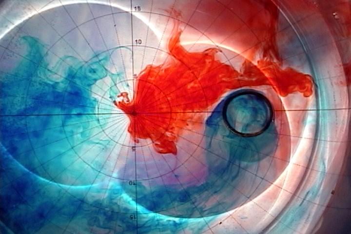
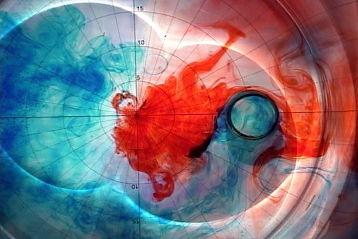
10 The CSU Spin Tank The Taylor-Proudman Theorem can be demonstrated beautifully by means of spin-tank experiments. A Spin-tank or rotating dish-pan has been constructed at Colorado State University to demonstrate various geophysical fluid phenomena. It was built with a small budget ($3000) and is portable. 5

11 The CSU Spin Tank The Taylor-Proudman Theorem can be demonstrated beautifully by means of spin-tank experiments. A Spin-tank or rotating dish-pan has been constructed at Colorado State University to demonstrate various geophysical fluid phenomena. It was built with a small budget ($3000) and is portable. A description of the spin-tank at CSU is given at mcnoldy/spintank/ At this site, a number of experiments are described. There are several MPEG loops showing the results of these experiments. See also the article in Bull. Amer. Met. Soc., December, This Journal is freely available online. 5

12 Taylor-Proudman Column Schematic diagram of tank Taylor-Proudman Column 6

13 7

14 8

15 9

16 Simple Steady-state Solutions 10

17 Polar Coordinates The flow will be assumed to be axially or circularly symmetric, and it is convenient to introduce (cylindrical) polar coordinates. 11

18 Polar Coordinates The flow will be assumed to be axially or circularly symmetric, and it is convenient to introduce (cylindrical) polar coordinates. Let R and θ be the radial distance and azimuthal angle. Let U and V be radial and azimuthal components of velocity. 11

19 Axially Symmetric Steady Flow We will study some steady-state or time-independent solutions. 12

20 Axially Symmetric Steady Flow We will study some steady-state or time-independent solutions. We assume that the radial velocity vanishes: U 0. We assume a steady state: V t = 0, We assume axial symmetry: V θ = 0, p t = 0. p θ = 0. 12

21 Axially Symmetric Steady Flow We will study some steady-state or time-independent solutions. We assume that the radial velocity vanishes: U 0. We assume a steady state: V t = 0, We assume axial symmetry: V θ = 0, p t = 0. p θ = 0. Definition: Flow with fv > 0 is called cyclonic. Flow with fv < 0 is called anticyclonic. 12

22 Axially Symmetric Steady Flow We will study some steady-state or time-independent solutions. We assume that the radial velocity vanishes: U 0. We assume a steady state: V t = 0, We assume axial symmetry: V θ = 0, p t = 0. p θ = 0. Definition: Flow with fv > 0 is called cyclonic. Flow with fv < 0 is called anticyclonic. Exercise: Show that cyclonic motion spins in the same sense as the earth, and anti-cyclonic motion spins in the opposite sense. 12

23 Some Vector Calculus For polar (cylindrical) coordinates, we have Φ = Φ R i + 1 Φ ( R θ j 1 (RU) V = R R + 1 ) V ( R θ 1 (RV ) k V = R R 1 ) U R θ 13

24 Some Vector Calculus For polar (cylindrical) coordinates, we have Φ = Φ R i + 1 Φ ( R θ j 1 (RU) V = R R + 1 ) V ( R θ 1 (RV ) k V = R R 1 ) U R θ Since we have assumed U 0, the divergence and vorticity become δ V = 1 V R θ = 0 ζ k V = 1 (RV ) R R = V R + V R 13

25 Some Vector Calculus For polar (cylindrical) coordinates, we have Φ = Φ R i + 1 Φ ( R θ j 1 (RU) V = R R + 1 ) V ( R θ 1 (RV ) k V = R R 1 ) U R θ Since we have assumed U 0, the divergence and vorticity become δ V = 1 V R θ = 0 ζ k V = 1 (RV ) R R = V R + V R For solid body rotation, V = ωr where the angular velocity ω is constant. Then the vorticity becomes ζ = (ωr) R + ωr R = 2ω. 13

26 The directions of the unit vectors change with θ: i θ = j, j θ = i. 14

27 The directions of the unit vectors change with θ: i θ = j, j θ = i. The advection may be calculated: V = Ui + V j, so ( V V = U R + V ) (Ui + V j) ( R θ = U U R + V ) ( U i + U V R θ R + V ) V R θ +U 2 i R + UV i R θ + UV j R + V 2 j R θ. j 14

28 The directions of the unit vectors change with θ: i θ = j, j θ = i. The advection may be calculated: V = Ui + V j, so ( V V = U R + V ) (Ui + V j) ( R θ = U U R + V ) ( U i + U V R θ R + V ) V j R θ +U 2 i R + UV i R θ + UV j R + V 2 j R θ. When we assume azimuthal symmetry and vanishing radial velocity, all terms except the last one vanish: V V = V 2 R i. This is the usual expression for the centripetal acceleration. 14

29 The Coriolis term is fk V = fk (Ui + V j) = fv i + fuj. 15

30 The Coriolis term is fk V = fk (Ui + V j) = fv i + fuj. The pressure gradient force is 1 ρ p = 1 ( p ρ R i + 1 ) p R θ j or g h = g ( h R i + 1 ) h R θ j 15

31 The Coriolis term is fk V = fk (Ui + V j) = fv i + fuj. The pressure gradient force is 1 ρ p = 1 ( p ρ R i + 1 ) p R θ j or g h = g ( h R i + 1 ) h R θ j The balance of forces in the radial direction now becomes V 2 R h + fv g R = 0. In the azimuthal direction, all terms vanish. ( ) 15

32 The Coriolis term is fk V = fk (Ui + V j) = fv i + fuj. The pressure gradient force is 1 ρ p = 1 ( p ρ R i + 1 ) p R θ j or g h = g ( h R i + 1 ) h R θ j The balance of forces in the radial direction now becomes V 2 R h + fv g R = 0. In the azimuthal direction, all terms vanish. We will look at several solutions of (*). But first, we digress to consider Natural Coordinates. ( ) 15

33 Aside: Natural Coordinates Let s be a unit vector parallel to the velocity V, and let n be a unit vector perpendicular to s, pointing to its left. 16

34 Aside: Natural Coordinates Let s be a unit vector parallel to the velocity V, and let n be a unit vector perpendicular to s, pointing to its left. 16

35 Aside: Natural Coordinates Let s be a unit vector parallel to the velocity V, and let n be a unit vector perpendicular to s, pointing to its left. Let R be the radius of curvature of the streamline. If the centre of curvature is in the direction of n, we take R positive, and call the flow cyclonic. For R < 0, we call it anticyclonic flow. (NHS Convention) 16

36 We write the velocity as V = V s where V = ds/dt is the speed. Note that both V and s vary along the trajectory. Positive curvature (R > 0) means flow turning to the left. Negative curvature (R < 0) means flow turning to the right. Exercise: Show that ds ds = n R. 17

37 We write the velocity as V = V s where V = ds/dt is the speed. Note that both V and s vary along the trajectory. Positive curvature (R > 0) means flow turning to the left. Negative curvature (R < 0) means flow turning to the right. Exercise: Show that ds ds = n R. In a distance s along the curve, the flow turns through and angle θ = s/r. The unit vector s turns through the same angle, while its length remains unchanged. Therefore θ = s. Moreover, this gives s s = 1 R The direction of s is the same as n for positive R and opposite for negative R. Therefore ds ds = n R. which is the desired result. 17

38 The rate of change of s along the trajectory is ds ds = n R, so that ds dt = ds ds ds dt = V n R. 18

39 The rate of change of s along the trajectory is ds ds = n R, so that ds dt = ds ds ds dt = V n R. Then the acceleration is ( dv d(v s) dv = = dt dt dt s + V ds ) ( ) dv = dt dt s + V 2 R n. 18

40 The rate of change of s along the trajectory is ds ds = n R, so that ds dt = ds ds ds dt = V n R. Then the acceleration is ( dv d(v s) dv = = dt dt dt s + V ds ) ( ) dv = dt dt s + V 2 R n The balance of forces perpendicular to V is: V 2 R + fv + g h n = 0.. ( ) Equation (**) is equivalent to the result obtained above using polar coordinates. 18

41 The results in polar coordinates and natural coordinates must agree. However, they appear different, because the sign conventions are different. 19

42 The results in polar coordinates and natural coordinates must agree. However, they appear different, because the sign conventions are different. To avoid confusion, we state the conventions here: 19

43 The results in polar coordinates and natural coordinates must agree. However, they appear different, because the sign conventions are different. To avoid confusion, we state the conventions here: In Natural Coordinates: The quantity V (the speed) is always positive The radius of curvature R may be positive or negative 19

44 The results in polar coordinates and natural coordinates must agree. However, they appear different, because the sign conventions are different. To avoid confusion, we state the conventions here: In Natural Coordinates: The quantity V (the speed) is always positive The radius of curvature R may be positive or negative In Polar Coordinates: The quantity V may be positive or negative The radius R is always positive We will not use natural coordinates. They are described above because they appear in Holton s text. 19

45 Geostrophic Balance (Ro 1) The balance of forces perpendicular to V is: V 2 R + fv g h R = 0. 20

46 Geostrophic Balance (Ro 1) The balance of forces perpendicular to V is: V 2 R + fv g h R = 0. For synoptic flow, the centrifugal force is small: Thus, V 2 R fv Ro = V fr 1 ; V = V Geos g f h R This is a state of geostrophic balance, as discussed already. 20

47 Geostrophic Balance (Ro 1) The balance of forces perpendicular to V is: V 2 R + fv g h R = 0. For synoptic flow, the centrifugal force is small: Thus, V 2 R fv Ro = V fr 1 ; V = V Geos g f h R This is a state of geostrophic balance, as discussed already. The flow is cyclonic around low pressure and anticyclonic around high pressure. 20

48 Geostrophically balanced flow around low and high pressure. 21

49 Digression: Tidal Range in Irish Sea Within the Irish Sea, the maximum tidal ranges occur on the Lancashire and Cumbria coasts, where the mean spring tides have a range of 8m. At Carnsore Point, the range is less than 2m. 22

50 Morecambe Bay Morecambe Bay is broad and shallow and has a large tidal range of up to 10.5 metres. The Bay is always changing with waves, tides and currents moving sediment from the Irish Sea into the embayment. Muds and silts settle, forming banks and marshes, whose edges are shaped by wandering river channels. Shoreline Managament Plan 23

51 Cyclostrophic Balance (Ro 1) Recall the balance of forces perpendicular to V: V 2 R + fv g h R = 0. 24

52 Cyclostrophic Balance (Ro 1) Recall the balance of forces perpendicular to V: V 2 R + fv g h R = 0. Let us assume the Coriolis term is negligible: V 2 R g h R = 0 ; V = ± gr h R. 24

53 Cyclostrophic Balance (Ro 1) Recall the balance of forces perpendicular to V: V 2 R + fv g h R = 0. Let us assume the Coriolis term is negligible: V 2 R g h R = 0 ; V = ± gr h R. This is cyclostrophic balance. For V to be real, we must have h/ R > 0, i.e., low pressure at the centre! 24

54 Cyclostrophic Balance (Ro 1) Recall the balance of forces perpendicular to V: V 2 R + fv g h R = 0. Let us assume the Coriolis term is negligible: V 2 R g h R = 0 ; V = ± gr h R. This is cyclostrophic balance. For V to be real, we must have h/ R > 0, i.e., low pressure at the centre! The centrifugal force is much bigger than the Coriolis force: V 2 R fv, which implies Ro V 2ΩL = V fr 1. Cyclostrophic balance is found in small vortices. It may be cyclonic or anticyclonic. 24

55 Example: A Toy Tornado The centrifugal term is important in tornado dynamics. [1] Calculate the Rossby Number for typical scale values. [2] Calculate the variation of depth with radius. 25

56 Example: A Toy Tornado The centrifugal term is important in tornado dynamics. [1] Calculate the Rossby Number for typical scale values. [2] Calculate the variation of depth with radius. [1] We take the velocity and length scales to be V = 30 m s 1 and L = 300 m. Assuming f = 10 4 s 1, we have Ro V fl = = Almost every tornado is found to rotate cyclonically. However, there are documented cases of rotation in an anticyclonic direction. Smaller vortices such as dust devils are found to rotate indifferently in both directions. 25

57 [2] Let us assume solid-body rotation, ω = V/r constant. This is not very realistic, but is done to simplify the analysis. 26

58 [2] Let us assume solid-body rotation, ω = V/r constant. This is not very realistic, but is done to simplify the analysis. The balance of forces (Centrifugal = Pressure Gradient) gives V 2 R g h R = 0 or ω2 R g h R = 0. 26

59 [2] Let us assume solid-body rotation, ω = V/r constant. This is not very realistic, but is done to simplify the analysis. The balance of forces (Centrifugal = Pressure Gradient) gives V 2 R g h R = 0 or ω2 R g h R = 0. This gives the pressure gradient: h R = ω2 g R and we can integrate this from 0 to R to get h = h 0 + ω2 2g R2 which is a parabolic profile. This completes the solution. 26

60 [2] Let us assume solid-body rotation, ω = V/r constant. This is not very realistic, but is done to simplify the analysis. The balance of forces (Centrifugal = Pressure Gradient) gives V 2 R g h R = 0 or ω2 R g h R = 0. This gives the pressure gradient: h R = ω2 g R and we can integrate this from 0 to R to get h = h 0 + ω2 2g R2 which is a parabolic profile. This completes the solution. Stir your coffee rapidly. Study the shape of the surface. 26

61 Exercise: Down the Plug-hole A popular legend holds that water draining from a bath spins cyclonically, that is, counter-clockwise in the northern hemisphere. Show that this is a myth. 27

62 Exercise: Down the Plug-hole A popular legend holds that water draining from a bath spins cyclonically, that is, counter-clockwise in the northern hemisphere. Show that this is a myth. We take the velocity and length scales to be V = 1 m s 1 and L = 1 m. Assuming f = 10 4 s 1, we have Ro V fl = = Thus, the Coriolis effect is completely negligible at this scale: Coriolis force Centrifugal force 27

63 Exercise: Down the Plug-hole A popular legend holds that water draining from a bath spins cyclonically, that is, counter-clockwise in the northern hemisphere. Show that this is a myth. We take the velocity and length scales to be V = 1 m s 1 and L = 1 m. Assuming f = 10 4 s 1, we have Ro V fl = = Thus, the Coriolis effect is completely negligible at this scale: Coriolis force Centrifugal force Experiments confirm that the two spin directions are equally likely. The balance in the bath is cyclostrophic, not geostrophic. 27

64 Exercise: Down the Plug-hole A popular legend holds that water draining from a bath spins cyclonically, that is, counter-clockwise in the northern hemisphere. Show that this is a myth. We take the velocity and length scales to be V = 1 m s 1 and L = 1 m. Assuming f = 10 4 s 1, we have Ro V fl = = Thus, the Coriolis effect is completely negligible at this scale: Coriolis force Centrifugal force Experiments confirm that the two spin directions are equally likely. The balance in the bath is cyclostrophic, not geostrophic. Extremely delicate laboratory conditions are required to achieve a preference for cyclonic rotation on the bathroom scale. 27

65 Inertial Balance Once more, the balance of forces is: V 2 R + fv g h R = 0. 28

66 Inertial Balance Once more, the balance of forces is: V 2 R + fv g h R = 0. If the pressure force is neglected, we get V 2 + fv = 0, which implies V = fr. R This is inertial flow. Since, by convention, R > 0 we must have fv < 0. That is, inertial flow is anticyclonic. 28

67 Inertial Balance Once more, the balance of forces is: V 2 R + fv g h R = 0. If the pressure force is neglected, we get V 2 + fv = 0, which implies V = fr. R This is inertial flow. Since, by convention, R > 0 we must have fv < 0. That is, inertial flow is anticyclonic. The angular velocity is independent of radius: ω = V/R = f. This implies solid body rotation. The period for revolution is T = 2π f 17.5 hours at 45 N. This is the time taken by a Foucault Pendulum to rotate through 180 and is called a half pendulum day. 28

68 Inertial oscillations are relatively unimportant in the atmosphere, where pressure gradients are rarely negligible, but are more important in the ocean. 29

69 Inertial oscillations are relatively unimportant in the atmosphere, where pressure gradients are rarely negligible, but are more important in the ocean. They are normally superimposed on a background flow, leading to cycloidal patterns such as shown below. 29

70 Gradient Balance When all terms are retained, we have Gradient balance: V 2 R + fv g h R = 0. 30

71 Gradient Balance When all terms are retained, we have Gradient balance: V 2 R + fv g h R = 0. Using the definition of geostrophic wind V Geos = (g/f) h/ R, this becomes V 2 R + f(v V Geos) = 0. ( ) 30

72 Gradient Balance When all terms are retained, we have Gradient balance: V 2 R + fv g h R = 0. Using the definition of geostrophic wind V Geos = (g/f) h/ R, this becomes V 2 R + f(v V Geos) = 0. ( ) We may solve this quadratic equation for the wind speed: V = 1 [ ] fr ± f 2 2 R 2 + 4fRV Geos. 30

73 Gradient Balance When all terms are retained, we have Gradient balance: V 2 R + fv g h R = 0. Using the definition of geostrophic wind V Geos = (g/f) h/ R, this becomes V 2 R + f(v V Geos) = 0. ( ) We may solve this quadratic equation for the wind speed: V = 1 [ ] fr ± f 2 2 R 2 + 4fRV Geos. For a given pressure gradient, there are two possible solutions, one regular and one anomalous. Not all solutions are physically possible. 30

74 Gradient Balance When all terms are retained, we have Gradient balance: V 2 h + fv g R R = 0. Using the definition of geostrophic wind V Geos = (g/f) h/ R, this becomes V 2 R + f(v V Geos) = 0. ( ) We may solve this quadratic equation for the wind speed: V = 1 [ ] fr ± f 2 2 R 2 + 4fRV Geos. For a given pressure gradient, there are two possible solutions, one regular and one anomalous. Not all solutions are physically possible. N.B. A strong anticyclonic gradient h/ R 0 implies fv Geos 0 so that V is complex. Strong gradients are not found near high pressure centres in the atmosphere. 30

75 For cyclonic flow the gradient wind speed is less than the geostrophic speed; for anti-cyclonic flow it is greater. This follows from (*): V = V Geos V 2 fr. So, Cyclonic flow (fv > 0): V < V Geos (Sub-geostrophic) Anticylonic flow (fv < 0): V > V Geos (Super-geostrophic) 31

76 For cyclonic flow the gradient wind speed is less than the geostrophic speed; for anti-cyclonic flow it is greater. This follows from (*): V = V Geos V 2 fr. So, Cyclonic flow (fv > 0): V < V Geos (Sub-geostrophic) Anticylonic flow (fv < 0): V > V Geos (Super-geostrophic) Exercise: Show that, for a given wind speed, the pressure gradient is greater when the flow is cyclonic, and less when the flow is anti-cyclonic. Discuss the implications of this for synoptic analysis. For a more comprehensive discussion of gradient balance, read Holton, Chapter 3. 31

77 Exercises (1) Download a weather chart with isobars and winds. Study how the flow direction and speed depend on the pressure gradient. Locate a similar map for the southern hemisphere. Find a similar map for the tropics. How are the pressure and wind fields related near the equator? 32

78 Exercises (1) Download a weather chart with isobars and winds. Study how the flow direction and speed depend on the pressure gradient. Locate a similar map for the southern hemisphere. Find a similar map for the tropics. How are the pressure and wind fields related near the equator? (2) Search for Coriolis Force. Look for animations that show the effect of this deflecting force. 32

79 Exercises (1) Download a weather chart with isobars and winds. Study how the flow direction and speed depend on the pressure gradient. Locate a similar map for the southern hemisphere. Find a similar map for the tropics. How are the pressure and wind fields related near the equator? (2) Search for Coriolis Force. Look for animations that show the effect of this deflecting force. (3) Search for an example of an anomalous tornado, that is, a tornado with anticyclonic circulation. Does it differ in any way from the usual cyclonic tornadoes? 32

80 Exercises (1) Download a weather chart with isobars and winds. Study how the flow direction and speed depend on the pressure gradient. Locate a similar map for the southern hemisphere. Find a similar map for the tropics. How are the pressure and wind fields related near the equator? (2) Search for Coriolis Force. Look for animations that show the effect of this deflecting force. (3) Search for an example of an anomalous tornado, that is, a tornado with anticyclonic circulation. Does it differ in any way from the usual cyclonic tornadoes? (4) Visit the site describing the CSU Spin-tank mcnoldy/spintank/ and study the movie loops there. 32