Applications of Geometry in Optimization and Statistical Estimation

Transcription

1 Applications of Geometry in Optimization and Statistical Estimation by Vahed Maroufy A thesis presented to the University of Waterloo in fulfillment of the thesis requirement for the degree of Doctor of Philosophy in Statistics Waterloo, Ontario, Canada, 2015 c Vahed Maroufy 2015

2 Author s Declaration I hereby declare that I am the sole author of this thesis. This is a true copy of the thesis, including any required final revisions, as accepted by my examiners. I understand that my thesis may be made electronically available to the public. ii

3 Abstract Geometric properties of statistical models and their influence on statistical inference and asymptotic theory reveal the profound relationship between geometry and statistics. This thesis studies applications of convex and differential geometry to statistical inference, optimization and modeling. We, particularly, investigate how geometric understanding assists statisticians in dealing with non-standard inferential problems by developing novel theory and designing efficient computational algorithms. The thesis is organized in six chapters as it follows. Chapter 1 provides an abstract overview to a wide range of geometric tools, including affine, convex and differential geometry. It also provides the reader with a short literature review on the applications of geometry in statistical inference and exposes the geometric structure of commonly used statistical models. The contributions of this thesis are organized in the following four chapters, each of which is the focus of a submitted paper which is either accepted or under revision. Chapter 2 introduces a new parametrization to general family of mixture models of the exponential family. Despite the flexibility and popularity of mixture models, their associated parameter spaces are often difficult to represent due to fundamental identification problems. Other related problems include the difficulty of estimating the number of components, possible unboundedness and non-concavity of the log-likelihood function, non-finite Fisher information, and boundary problems giving rise to non-standard analysis. For instance, the order of a finite mixture is not well defined and often can not be estimated from a finite sample when components are not well separated, or some are not observed in the sample. We introduce a novel family of models, called the discrete mixture of local mixture models, which reparametrizes the space of general mixtures of the exponential family, in a way that the parameters are identifiable, interpretable, and, due to a tractable geometric structure, the space allows fast computational algorithms. This family also gives a well-defined characterization to the number of components problem. The component densities are flexible enough for fitting mixture models with unidentifiable components, and our proposed algorithm only includes the components for which there is iii

4 enough information in the sample. This paper is under revision in Statistics and Computing Journal. Chapter 3 uses geometric concepts to characterize the parameter space of local mixture models (LMM), introduced in Marriott (2002) as a local approximation to continuous mixture models. Although LMMs are shown to satisfy nice inferential properties, their parameter space is restricted by two types of boundaries, called the hard boundary and the soft boundary. The hard boundary guarantees that an LMM is a density function, while the soft boundary ensures that it behaves locally in a similar way to a mixture model. The boundaries are shown to have particular geometric structures that can be characterized by geometry of polytopes, ruled surface and developable surfaces. As working examples the LMM of a normal model and the LMM of a Poisson distribution are considered. The boundaries described in this chapter have both discrete aspects, (i.e. the ability to be approximated by polytopes), and smooth aspects (i.e. regions where the boundaries are exactly or approximately smooth). A version of this chapter has been published in Geometric Science of Information, Lecture Notes in Computer Science, p Chapter 4 uses the model space introduced in Chapter 2 for extending a prior model and defining a perturbation space in the Bayesian sensitivity analysis. This perturbation space is well-defined, tractable, and consistent with the elicited prior knowledge, the three properties that improve the methodology in Gustafson (1996). We study both local and global sensitivity in conjugate Bayesian models. In the local analysis the worst direction of sensitivity is obtained by maximizing the directional derivative of a functional between the perturbation space and the space of posterior expectations. For finding the maximum global sensitivity, however, two criteria are used; the divergence between posterior predictive distributions and the difference between posterior expectations. Both local and global analyses lead to optimization problems with a smooth boundary restriction. Work from this chapter is in a paper under revision in Statistics and Computing Journal. Chapter 5 studies Cox s proportional hazard model with an unobserved frailty for which no specific distribution is assumed. The likelihood function, which has a mixture structure with an unknown mixing distribution, is approximated by the model introduced in Chapter 2, which is always identifiable and estimable. The nuisance parameters in the approximativ

5 ing model, which represent the frailty distribution through its moments, lie in a convex space with a smooth boundary, characterized as a smooth manifold. Using differential geometric tools, a new algorithm is proposed for maximizing the likelihood function restricted by the smooth yet non-trivial boundary. The regression coefficients, the parameters of interest, are estimated in a two step optimization process, unlike the existed methodology in Klein (1992) which assumes a gamma assumption and uses Expectation-Maximization approach. Simulation studies and data examples are also included, illustrating that the new methodology is promising as it returns small estimation bias; however, it produces larger standard deviation compared to the EM method. The larger standard deviation can be the result of using no information about the shape of the frailty model, while the EM model assumes the gamma model in advance; however, there are still ways to improve this methodology. Also, the simulation section and data analysis in this chapter is rather incomplete and more work needs to be done. Chapter 6 outlines a few topics as future directions and possible extensions to the methodologies developed in this thesis. v

6 Acknowledgements Although my name is alone on the front cover of this dissertation, I am by no means its sole contributor. Rather, there are a number of people behind this piece of work who deserve my greatest thanks and appreciation. First and foremost, my sincere gratitude goes to my supervisor, Prof. Paul Marriott, for his inspiring guidance, kindness, and generosity. Without him this work would never have been possible. His support went far beyond technical insights into geometry and statistics and financial support; he lead me to a more rational and less stressful academic life. I learned from him how to work in a group with courage, patience and mutual respect, how to stay on my feet after disappointments, and how to learn from mistakes. I would also like to extend my gratitude to Prof. Christopher Small, as my presence at the University of Waterloo was due to his kindness, generosity and trust in me. To my thesis committee, Prof. Shinto Eguchi at Institute of Statistical Mathematics, Tokyo, Prof. Pengfei Li, Prof. Martin Lysy, Prof. Tony Wirjanto and Prof. Dinghai Xu, at University of Waterloo, for their insightful comments on the earlier version of this thesis. Thank you to all the faculty members and staff of the department of Statistics and Actuarial science for accepting me as a member of such a wonderful and friendly family. Special mention to Mary Lou Dufton, Lucy Simpson, Marg Feeney, Karen Richardson, and Anthea Dunne, who had answers to all my administrative inquiries and solutions to all the problems. I would also like to thank my best friends Reza Ramezan, Gwyneth Ramezan, Kadir Mirza, Amirhosein Vakili and Sina Hajitaheri for being my true family in Canada- for being there with me at all the tough moments and for all the fun and memorable times we had during these years. Finally, the biggest sacrifice I made to make this happen was to move away from my closest loved ones: my loving, strong, and protective parents Rahim Maroufy and Soda Ahmadzadeh, and my funny, generous and supportive brothers Ahad, Farhad, and Mohammad. I am forever indebted to them and I want to thank them for all the encouragement, love, and emotional support they provided me throughout my life. vi

7 To my parents Rahim and Soda who taught me the first lessons about life. I could never have done this without your support and encouragement. and my three cherished brothers Ahad, Farhad and Mohammad, without you my life would be boring and incomplete. vii

8 Contents Author s Declaration Abstract Acknowledgements Dedication List of Tables List of Figures ii iii vi vii xi xii 1 Convex and Differential Geometry in Statistics Introduction Geometry in Statistics Affine Spaces Convex Geometry Polyhedrons Ruled Surfaces and Developable Surfaces Envelope of a Family of Planes viii

9 1.6 Differential Geometry Statistical Manifold Tangent Spaces Metric Tensors Affine connections Statistical Examples Exponential Family Extended exponential Family Mixture Family Local Mixture Models Log-linear Models Summary and Contributions Mixture Models: Building a Parameter Space Introduction Background The Local Mixture Approach Local and Global Mixture Models Choosing the Support Points Estimation Methods Summary and Contributions Supplementary materials and proofs Orthogonal projection ix

10 3 Computing Boundaries in Local Mixture Models Introduction Local Mixture Models Computing the boundaries Hard Boundary for the LMM of Poisson distribution Hard Boundary for the LMM of Normal Soft Boundary calculations Summary and Contributions Supplementary materials and proofs Approximating general boundaries Profile Likelihood Simulation Proofs More on Hard Boundaries Surface Parametrization and Optimization Local and global robustness in conjugate Bayesian analysis Introduction Perturbation Space Theory and Geometry Prior Perturbation Local Sensitivity Global sensitivity Estimating λ Examples x

11 4.7 Summary and Contributions Supplementary materials and proofs Positivity Conditions Proofs Generalizing the Frailty Assumptions in Survival Analysis Introduction Methodology Local Mixture Method Maximum Likelihood Estimator for λ Non-parametric Hazard Simulation Study Example Summary and Contributions Supplementary materials and proofs The Algorithm Description Proofs Discussion and Future Work Discussion Future Work Hypothesis Testing for Mixture of LMMs Inference on Log-linear and Graphical Models Over-dispersion in Count data References 103 xi

12 List of Tables 2.1 Further analysis for different values of γ Bias and standard deviation of coefficient estimates, when frailty is generated from Γ( 1, η) η 5.2 Bias and standard deviation of coefficient estimates, when frailty is generated from Γ( 1, η). λ and β are iterated until convergence η 5.3 Coefficient estimates for placebo group of rhdnase data using both methods with unspecified hazard function are obtained Coefficient estimates for the treatment group of rhdnase data xii

13 List of Figures 1.1 A cone, a cylinder and a ruled surface (right), which is not a developable surface, formed by α(x) and β(x) = α (x) + e 3, where e 3 = (0, 0, 1) Tangential developable Ruled surface of a two-by-two contingency table inside 3D simplex Left, the QQ-plot for samples generated from each finite mixture model. Right: the histogram of the sample with fitted local mixture density plots for each sample Discrete mixture of LMMs for Acidity data Left to right: three and four components fit corresponding to the last three rows in Table The density (left) and distribution function (middle) plots of φ(x, µ, 1) (blue dash line) and and g µ,µ0 (x) (red solid line), for µ 0 = 0 and µ = 0.6. Right panel; the difference between the two distribution functions Left: slice through λ 2 = 0.1; Right: slice through λ 3 = 0.3. Solid lines represent active and dashed lines redundant constraints. For our model λ 4 > 0 is a necessary condition for positivity Left: The hard boundary for the normal LMM (shaded) as a subset of a self intersecting ruled surface (unshaded); Right: slice through λ 4 = xiii

14 3.3 Left: the 3-D curve ϕ(µ); Middle: the bounding ruled surface γ a (µ, u); Right: the convex subspace restricted to soft boundary t = 10, 5, 2, 1, 0.9, 0.7 presented by red, blue, black, green, purple, gray dashed (black) line presents N(µ, 1) and dash-dot (blue) the likelihood for N(µ, ˆσ). For the panel on left ˆλ is a interior point estimate, while in the panel on right it is boundary point estimate Left panel: gives a schematic graph for the proof. Middle and right panel present actual lines representing the boundary planes for a fixed λ 3 < 0 and a fixed λ 3 > 0, respectively dimensional slices of Λ µ through λ 2 = 0.1. Left: LMM of Bin(100, 3.5), the dashed lines represent the planes for x 50. Right: Bin(10, 3.5), and the planes for x = 1, 2, 3, 4, 5 are redundant in this slice Different angles of Λ µ Different slices through λ Different slices through λ The hard boundary for σ = 1 (blue) vs σ = 1.2 (red) Different angles of Λ µ for f(x, µ) = µ e µx Different slices through λ 4, for f(x, µ) = µ e µx A schematic graph for visualizing the orthogonal reparametrization Contour plat of the loglikelihood function on the boundary surface D. Left: for 1 < x 0 < 1 where x 0 = 0, represents the cusp in the edge of regression. Middle: for x 0 > 1. Right: the whole surface where it splits as the result of the two asymptotes at x 0 = ± respectively, plots for sample, and posterior densities of the based (solid) and perturbed (dashed) model corresponding to ˆλ Ψ Posterior density displacement corresponding to λ = αˆλ ϕ for α = 0.1, 0.15, 0.25 and the boundary point at the maximum direction xiv

15 4.3 (a),(b) correspond to ˆλ Ψ and ˆλ D, under λ 1 = 0, respectively, including the base (solid) and perturbed posterior (dashed). (c) presents posterior densities of based model (Base), and perturbed models for ˆλ Ψ (Rst psi) and ˆλ D (Rst KL) under λ 1 = 0, and the full perturbed posterior model (Full pert) from Example (a)-(e) posterior densities of based models and perturbed model (dashed) corresponding to λ = αˆλ ϕ where α = 0.05, 0.07, 0.1, 0.13, 0.15 and (f) for boundary point in direction of ˆλ ϕ (a)-(e) posterior densities of based models and perturbed model (dashed) corresponding to λ = αˆλ ϕ where α = 0.05, 0.07, 0.1, 0.13, 0.15 and (f) for boundary point in direction of ˆλ ϕ Presents all the perturbed prior models in Example 4.1 (Prior4), Example 4.2 (Prior3 and PriorKL for ˆλ Ψ and ˆλ D ) and Example 4.3 (Prior2) First row: estimates from the base model; second row: estimates form the perturbed model Schematic visualization of the algorithm steps xv

16 Chapter 1 Convex and Differential Geometry in Statistics 1.1 Introduction Geometric methods are frequently applied in statistics since various geometric concepts such as vector spaces, affine spaces, manifolds, polyhedrons and convex hulls commonly appear in statistical theory (Amari, 1985; Lindsay, 1995). The application of differential geometry to statistics was inaugurated by Rao (1945), Jeffreys (1946) and Efron (1975), then explicitly formulated by Amari (1985), Eguchi (1985), Barndorff-Nielsen (1987b) and Critchley et al. (1993). Essentially, a family of parametric models is characterized as a manifold on which a suitable geometry is imposed using tensors based on statistical objects such as the Fisher information. More applications of these approaches to statistical modeling and asymptotic theory can be found in Eguchi (1985, 1991), Barndorff-Nielsen (1988), Murray and Rice (1993), Critchley et al. (1994), Marriott and Salmon (2000) and Marriott (2002). In addition, convex geometry tools have been applied to the maximum likelihood estimation in mixture models (Lindsay, 1995), extended exponential family and log-linear models (Fienberg and Rinaldo, 2012; Eriksson et al., 2006), and graphical models (Wainwright and Jordan, 2006; Peng et al., 2012). 1

17 This introductory chapter intends to give an abstract overview of applications of geometry to statistics, and reviews the geometric tools necessary for developing the statistical theories and computational algorithms presented throughout this thesis. The chapter is organized as follows. Section 1.2 is an abstract review on the applications of differential and convex geometry in statistics. Section 1.3, introduces affine spaces and studies two important affine spaces in statistical theory. These spaces play an instrumental role in developing latter sections where we define a statistical manifold as an embedded manifold into an affine space, and define its geometry from the geometry of the affine spaces. Section 1.4 is a short overview on the theory of convex spaces, specifically cones and polyhedrons. Section 1.5 studies two specific surfaces: ruled surfaces and developable surfaces which are shown to be useful in characterizing the boundary of certain convex spaces in Chapter 3. Section 1.6 is devoted to differential geometry theory, where a statistical manifold is defined by embedding a parametric model into an affine space, and the required geometric concepts such as tangent spaces, metric tensors and affine connections, are explicitly defined. Finally, the chapter closes with Section 1.7, covering a number of commonly used statistical models and their essential geometric properties. 1.2 Geometry in Statistics Differential and convex Geometry have been applied to statistical inference theory of commonly used statistical families, such as the exponential family, the mixture and local mixture family, log-linear and graphical models (Section 1.7). Efron (1975) introduces the statistical curvature of one-dimensional models, and studies its influence on statistical inference and efficiency. For example, exponential families have nice inferential properties due to zero statistical curvature inside the exponential affine space (Section 1.3), while non-exponential models have non-zero statistical curvature, hence their asymptotic theory is not as tractable. For higher-dimensional models Murray and Rice (1993, p.18) provide a similar criterion, which is called the second fundamental form, obtained by the orthogonal component of the derivative of score functions to the tangent space. Amari (1985, ch.4) studies the asymptotic theory of inference in a curved exponential model when seen as a submanifold embedded in the exponential family. The geometry of the embedded manifold 2

18 is obtained from the larger manifold and used to derive the joint asymptotic probability function of the maximum likelihood estimator (MLE) and associated ancillary statistics, as well as the conditional probability function of MLE given the ancillary, in the form of Edgeworth expansions. He also provides a geometric interpretation for consistency, first, second and third order efficiency of an estimator and shows that the MLE is consistent, first and second order efficient, and the bias corrected MLE is third order efficient (Amari, 1985, ch.5-8). Further results of this type can be found in Eguchi (1983), using minimum contrast geometry, in Barndorff-Nielsen (1986a), Barndorff-Nielsen et al. (1986), Barndorff-Nielsen (1987a), Barndorff-Nielsen (1987b) and Barndorff-Nielsen (1988) using observed information geometry, and in Marriott (1989) and Critchley et al. (1993) using preferred-point geometry. In addition, Critchley and Marriott (2014) show how embedding statistical models in a simplex generalizes the above geometries to statistical models that are not manifolds because of boundary restrictions, and study the behavior of their likelihood functions close to the boundaries. Studying the geometric aspects of the mixture family and local mixture family, such as convexity and flatness with respect to a suitable geometry, is also of great importance in exploiting the flexibility of these families in statistical inference and modeling (Amari, 1985; Lindsay, 1995; Marriott, 2002). In Lindsay (1995, ch.5), nonparametric maximum likelihood estimation (NPMLE) theorem estimates the mixing distribution by a unique nonparametric discrete distribution with a number of support points not more than the sample size. Essentially, a concave likelihood function is maximized over a convex feasible space of distributions which is defined by the convex hull of the unicomponent likelihood curve. Marriott (2002) and Anaya-Izquierdo and Marriott (2007a) study the local geometry of mixture models and show that a family of continuous mixture models with relatively small mixing variation can be approximated by a finite dimensional family to an arbitrary order. The approximating family, called the local mixture family, is a union of convex subspaces inside the mixture affine space (Section 1.3). These models are extended in Marriott (2006) and applied to information recovery and sensitivity analysis in Marriott and Vos (2004) and Critchley and Marriott (2004). Understanding the geometry of convex polyhedrons is the key to maximum likelihood 3

19 estimation in log-linear models. Eriksson et al. (2006) shows that in hierarchical log-linear models, MLE exists, if and only if, the observed vector of margins lies in the interior of the marginal cone. Fienberg and Rinaldo (2012) and Rinaldo et al. (2009) develop similar results under the conditional Poisson sampling scheme. Using the theory of the extended exponential family, they derive the necessary and sufficient conditions for the existence of MLE, which depend on the sampling zeros in the observed table. They also provide an algorithm to obtain the extended MLE, which requires characterization of the boundary of the marginal cone using the geometry of faces, projection cones and normal cones. Their algorithm has two major steps; first, a unique face of a possibly low-dimensional polyhedron, on which the observed vector of margin lies, is obtained by repetitive linear programing; second, the loglikelihood is restricted to the face and maximized. Parameter estimation in undirected graphical models is also a problem of optimizing an objective function on a marginal polytope. In some recent related works (Sontag and Jaakkola, 2007; Wainwright and Jordan, 2006; Peng et al., 2012) graphical models with cycles (i.e., not trees) are considered in which their marginal polytopes are not tractable. They replace the marginal polytope with an outer polytope or a semi-definite bound, then use a cutting plane algorithm for maximizing the objective function. 1.3 Affine Spaces This section intends to give a brief overview of affine spaces and an introduction to two important affine spaces in statistics. The affine property leads to a nice inference and asymptotic theory of statistical models, for example in the exponential family (Murray and Rice, 1993). Definition 1.1 A geometrical space, (X, V, +), consists of a set X, a vector space V and a translation operation + is called an affine space if x X and v 1, v 2 V, x + v 1 X and (x + v 1 ) + v 2 = x + (v 1 + v 2 ) and x 1, x 2 X v V such that x 1 + v = x 2. 4

20 In the following examples we review the two important affine spaces in statistical theory; the exponential affine space and mixture affine space. The earlier includes the exponential family as an affine subspace, while the later includes the mixture family with latent parameterization (Section 1.7.3) and the local mixture family. Also, both spaces contain the space of smooth densities as a subset and give a way of characterizing families of parametric models as embedded manifolds by embeddings θ log f(x; θ) and θ f(x; θ), respectively (Murray and Rice, 1993, ch.4; Marriott, 2002). Example 1.1 The exponential affine space is the triplet (M, V e, ), where M is the space of all positive measures up to a positive finite scale, absolutely continuous with respect to a measure, i.e, all have the same support S, V e = {g(x) g C (S, R)}, and is the transformation that for any p M and g V e returns p g = p e g. Example 1.2 The triplet (X m, V m, +) is called mixture affine space in which { } { } X m = g(x) g(x) dτ = 1, V m = g(x) g(x) dτ = 0, for a measure τ on the support S, and + is the usual addition of functions. In Murray and Rice, 1993 the exponential affine space is used as the embedding manifold for a family of smooth density functions, and its simple geometry is exploited to define a geometry on the embedded family by projection. Marriott (2002) embeds a smooth family f(x; θ) in the mixture affine space and gives a local approximation to a family of continuous mixture models of f(x; θ) by a convex subspace of the linear embedding space at each point θ. This local approximation subspace is called the family of local mixture models, which has nice inferential properties (Section 1.7.4). 1.4 Convex Geometry Convex sets, in their general and specific forms, such as convex hulls, polytopes and polyhedral cones, arise in statistical inference theory frequently (Section 1.2). This section 5

21 reviews the geometry of convex sets of different kinds and their related properties to statistical theory. Most of the definitions and theorems are taken from Berger (1987) and Matousek (2002). For basic geometric concepts such as hyperplane, half-space, open and close sets, distance, metric space refer to the aforementioned references and Bonnesen and Fenchel (1987). Throughout this section, by cones, polyhedrons and polytopes we shall mean the convex form of them. Definition 1.2 A subset C of an affine space A is called convex if tx + (1 t)y C for any x, y C and t [0, 1]. A function f : C R is called strictly convex if for any x, y C and γ [0, 1] we have f(γx + (1 γ)y) < γf(x) + (1 γ)f(y). Also, f is concave if f is convex. A common example of a convex set is the convex hull of a set of points (or any subset B A) which is defined as the smallest convex set containing all the points (subset B). Half-spaces and their intersections are also examples of convex sets. The dimension of a non-empty convex set C, dimc, is defined by the dimension of the affine subspace C, the smallest linear subspace containing C, called the subspace spanned by C. Thus, C A is called full-dimensional if dim C = dima. Also, by imposing a suitable metric on A, the distance between C and any point y A is defined by min{d(x, y); x C}, for which following result holds. Theorem 1.1 Suppose C is a convex set in an Euclidean affine space E, and x E, then there exists at most one point y C such that d(x, y) = min{d(x, z) z C}, where d(, ) is the Euclidean distance. An alternative way for characterizing convex closed sets is by supporting hyperplanes. Recall first that, for a vector u A and a constant v the hyperplane H = {x A x u = v} divides A into two half-spaces {x A x u v} and {x A x u v}, and two subsets B 1, B 2 A are said to be separated by the hyperplane H, if they lie in different half-spaces created by H. Definition 1.3 For a subset B of the affine space A, the supporting hyperplane of B at x B is defined as any hyperplane containing x and separating {x} from B. 6

22 A convex closed set C, with the boundary set shown by C, has at least one supporting hyperplane at any point of its boundary. Equivalently, a closed set with non-empty boundary is convex if it has at least one supporting hyperplane at any point of its boundary. The supporting hyperplanes can be used to classify the boundary points of convex sets. For instance, x C is a vertex if the intersection of all the supporting hyperplanes at x is an affine space of dimension zero, while C is said to be smooth at x if it has only one supporting hyperplane at x. (Bonnesen and Fenchel, 1987, p.15) Note also that any convex closed set can have only a countable number of vertices Polyhedrons Polyhedrons commonly arise in statistical inference of the extended exponential family and log-linear models in two specific forms; polytopes and polyhedral cones. Definition 1.4 A polyhedron is an intersection of a finitely many closed half-spaces, and a polytope is a bounded polyhedron. Equivalently, a polytope can be defined by the convex hull of a finite set of points. An important example of polytopes is a simplex which, for a given dimension, has the smallest number of vertices. A simplex is obtained by the convex hull of an affinely independent set of points. Recall that, a set of points are affinely independent if none of the points can be written as an affine combination of the rest of the points. The boundary of a polyhedron comprises vertices and higher-dimensional linear subspaces, which are all called faces of different orders, as characterized in the following definition. Definition 1.5 A face of a d-dimensional (2 d dima) polytope P is defined as P H, where H is a hyperplane and P is contained in one of the closed half-spaces determined by H. Specially, P is a face of itself called an improper face, vertices are 0-faces, and (d 1)-dim faces are called facets. An alternative criterion for characterizing a boundary point x of a polyhedron, is by the dimensionality of the polar cone at x. Specially, we can determine if x is vertex or a point in the interior of a face with the known dimensionality. 7

23 Definition 1.6 A cone C is a subset of a vector space such that for any two non-negative real numbers a, b and vectors v 1, v 2 C, we have av 1 + bv 2 C. The cone of a finite vector set V, cone(v ) called a polyhedral cone is defined by all the linear combinations with non-negative coefficients of vectors in V. Two important polyhedral cones, useful in describing the geometry of convex sets, are the projection cone and polar cone. The projection cone at any x C is cone(v x ), where V x is the set of all the rays emerging from x and containing another point of C. Polar cone of the projection cone at x, which is also called normal cone at x, is defined by cone(v Nx ) where V Nx is the set of normal vectors to all the supporting hyper-planes at x. The dimensionality of the cone(v Nx ) at x C determines the type of x. Specifically, if C is a d-dimensional closed convex set, then x is a vertex, a point on a p-face, or a point on a facet if dimensionality of cone(v Nx ) is, respectively, d, (d p) or (d 1). 1.5 Ruled Surfaces and Developable Surfaces In this section, two particular surfaces, ruled surfaces and developable surfaces, are briefly introduced. In Chapter 3 we illustrate the role of these surfaces in approximating the boundary of convex sets with some special geometric structures. The technical definitions and results are taken from Do Carmo (1976) and Struik (1988). Preliminary concepts such as regular curves and surfaces are available explicitly in Do Carmo (1976, ch.1,2). Intuitively, ruled surfaces are generated by a curve and a set of vectors, thus have more structure than a generic surface. A formal definition of ruled surfaces is as follows. Definition 1.7 A one-parameter family of lines {α(x), β(x)} is a correspondence that assigns to each x I R a point α(x) R 3 and a vector β(x) R 3, β(x) 0. For each x I the line L x, parallel to β(x) and passing through α(x), is called the line of the family at x. Given {α(x), β(x)}, the parametrized surface Γ(x, γ) = α(x) + γ β(x), x I, γ R. 8

24 is called the ruled surface generated by the family {α(x), β(x)}. Also, the lines L x are called rulings and the curve α(x) is called the directrix of Γ. If, in addition, β(x), β (x) and α (x) are coplanar for all x I, Γ(x, γ) is called a developable surface. Definition 1.7 can be generalized to higher dimensions by Γ(x, γ) = α(x) + γ β(x), x I, γ R k (1.5.1) where α(x) : R R k, β(x) R k, γ = (γ 1, γ 2,, γ k ) and γ β(x) = k i=1 γ iβ i (x). Clearly the geometric object defined by equation in (1.5.1) is not a surface or hyper-surface unless γ 1 = = γ k ; hence, we may call it a ruled space. Such spaces are simple examples of fiber bundles (Marriott, 2006). Example 1.3 Cylinders and Cones are the simplest ruled surfaces, and also developable surfaces. For a cylinder, α(x) is in a plane, say P, and the β(x) s are parallel to a fixed direction. A cone however is obtained from an α(x) P with rulings passing through a point p / P, called the vertex of the cone (Figure 1.1). Figure 1.1: A cone, a cylinder and a ruled surface (right), which is not a developable surface, formed by α(x) and β(x) = α (x) + e 3, where e 3 = (0, 0, 1) As illustrated in the definition, ruled surfaces consist of a curve and a set of straight lines attached to the curve, and developable surfaces are a specific form of ruled surfaces. Intuitively, a surface with vanishing Gaussian curvature, defined by determinant of the curvature matrix (Do Carmo, 1976, ch.3), at every point is a developable surface. Such surfaces are easily constructed by bending a plane without tearing and stretching (Sun and Fiume, 1996) and are widely used in many different areas of science and engineering. 9

25 1.5.1 Envelope of a Family of Planes One way of constructing a developable surface is by finding the envelope of a one-parameter family of planes. This idea can also be generalized to the envelope of a one-parameter family of general surfaces (Struik, 1988, Sec.2-4 and 5-1). For convenience in writing, we use λ = (λ 2, λ 3, λ 4 ) and a(x) = (a 1 (x), a 2 (x), a 3 (x)). Definition 1.8 The family of planes, A = {λ a(x) λ + d(x) = 0, x R}, in which a(x) and d(x) are differentiable, and each plane is determined by a value of the real parameter x, is called an infinite single parameter family of planes. Note that, Definition 1.8 can be generalized to a family of hyperplanes. Also, we exclude the family of parallel planes and the family forming a pencil, a family of planes passing through the same line. To obtain the envelope of the family A and give a similar geometric structure as that of ruled surfaces, we need to find the corresponding directrix and rulings. For any x 1,x 2 R the corresponding planes in A, under our mild regularity, intersect in a line called the characteristic line. If x 2 (x 1 ɛ, x 1 + ɛ) and ɛ 0, the intersecting line is obtained by the following equations, a(x 1 ) λ + d(x 1 ) = 0, a (x 1 ) λ + d (x 1 ) = 0 (1.5.2) In a similar way for any x 1,x 2,x 3 R the planes in A intersect in a point known as the characteristic point. If also x 3, x 2 belong to an ɛ interval of x 1, and ɛ 0, the characteristic point is determined by following equations, a(x 1 ) λ + d(x 1 ) = 0, a (x 1 ) λ + d (x 1 ) = 0, a (x 1 ) λ + d (x 1 ) = 0 (1.5.3) where, in equations (1.5.2) and (1.5.3), prime and double prime represent first and second derivatives with respect to x, respectively. Putting together the infinite number of characteristic points corresponding to the planes in the family A, we obtain a curve, called the edge of regression. Moreover, all the characteristic lines together, side-by-side, construct a surface called the envelope of the family 10

26 A, which is a developable surface (Figure 1.2). In addition, it can be shown that the characteristic lines are tangent to the edge of regression at their characteristic points, Struik (1988, p.67). Example 1.4 Another developable surface is tangential developable which is the envelope of a set of tangent planes to a space curve, L. Any plane P crossing L, intersects with the surface in a curve with a cusp on L; hence, edge of regression is also called cuspidal edge. The characteristic lines (rulings of the surface) are also tangent to L. edge of regression cusp Figure 1.2: characteristic line Tangential developable 1.6 Differential Geometry Differential geometry methods are shown to be instrumental in statistical theory, as under some regularity conditions a statistical model can form a Riemannian manifold equipped with Fisher information metric or observed information metric (Amari, 1985; Barndorff- Nielsen and Cox, 1989; Murray and Rice, 1993). This section provides an abstract overview of differential geometry methods required for the statistical applications in the following chapters. As in Murray and Rice (1993), a statistical manifold is defined by embedding a family of smooth densities into the exponential affine space and its geometric components are obtained with respect to the embedding affine space. We use these tools in the latter chapters where the boundary of (the fiber at a point) a convex parameter subspace is characterized as a smooth manifold immersed in an Euclidean space, and covariant derivatives are exploited to design a gradient-based searching algorithm on the manifold Statistical Manifold In differential geometry a manifold is defined in two different ways; as a space which is locally diffeomorphic to an open subspace of an Euclidean space at any point, or as a 11

27 non-linear space embedded into an affine space. Here we follow the second definition for two reasons. It is intuitive for statistical applications, as the set of density functions is a subset of the affine spaces in Section 1.3. Also, it is sufficient for our purposes throughout the thesis where we characterize the boundary of a convex parameter space as a manifold immersed in an Euclidean space. For formal definitions we follow Murray and Rice (1993) and Marriott and Salmon (2000) closely. Also, unless otherwise mentioned, for a family of densities f(x; θ), where θ = (θ 1,, θ r ), x = (x 1,, x d ), and l(θ; x) is the loglikelihood function, we assume the following regularity conditions, 1- All members have common support. 2- The set of functions { θ i l(θ; x) i = 1,, r} are linearly independent and their moments exists up to a sufficient order. 3- Integration and partial derivative for all relevant functions to f(x; θ) are commutative. The inverse function theorem (Dodson and Poston, 1979, p.221) and the implicit function theorem (Rudin, 1976, p.224) stated bellow, are also required for our definition of manifold to be concrete. Theorem 1.2 Suppose h : A A, where A and A are affine spaces and h C k, set of k times differentiable function. Then the derivative mapping at x, D x h, is an isomorphism, if and only if, there are neighborhoods N x and N h(x) of x and h(x) such that h(n x ) = N h(x) and h has a local C k inverse h 1 : N h(x) N x. Theorem 1.3 Suppose h is a continuously differentiable mapping from an open set U R m+n into R n such that, h(a, b) = 0 for some (a, b) U and D x h is invertible. Then there exist open sets U R m+n and W R m, with (a, b) U and b W such that, to every y W corresponds a unique x where (x, y) U and h(x, y) = 0. If x is defined by g(y), then g is a continuously differentiable mapping from W into R n, g(b) = a and h(g(y), y) = 0. Now we are at the position to define a manifold as the image of a smooth mapping into an affine space (Marriott and Salmon, 2000, p.17) as follows. Definition 1.9 For an open set Φ R r and affine space A, consider the map Υ : Φ A. Then the image Υ(Φ) is an embedded manifold if, 12

28 (i) the derivative of Υ has full rank r for all points in Φ, (ii) the inverse image of any compact set is itself compact. Condition (i) guarantees that Υ is invertible by Theorem 1.2, hence any point θ Φ has a unique image in A. Restriction (ii) is required so that the differential map of Υ is one-toone. Thus the image Υ(Φ) is locally diffeomorphic to a subset of R r, so it has a structure of a manifold on its own right, and also it is mapped into A by a closed inclusion. Recall that an inclusion from M( A) into A maps any point p M to the same point in A, and under a closed map the image of any closed set is a closed set. Although Definition 1.9 does not retain a global structure, this may not be an issue for applications in statistics as most of the statistical models only have one global coordinate; hence, they have one global differentiable chart (Amari, 1985, p.15). Definition 1.9 together with Example 1.1 give a way of expressing a family of smooth densities as an embedded manifold inside the exponential affine space. Note first that the exponential affine space can be presented via its logarithm representation by (M l, V e ) where M l = {log(p) p M}, and the translation is log(p) log(p) + f(x) This representation is more intuitive to work with as it is common to represent statistical manifolds by logarithm of density functions, and since a loglikelihood function is defined only up to addition of a constant, the space of loglikelihood functions is a natural subspace of M l. Now consider a family of smooth density functions satisfying the above regularity conditions embedded in the exponential affine space. The set of loglikelihoods of this family lie in M l, since by regularity condition 1 they have the same support. Condition (i) is immediately implied by regularity condition (2). For (ii) to be satisfied it amounts for the mapping to have a continuous inverse Tangent Spaces To apply geometric methods on a manifold, M, embedded in an affine space, A, a suitable geometric structure is required. The first step is to define the tangent space T M p at any 13

29 point p M. Tangent spaces can be defined in two different ways; as the best firstorder linear approximation of M about p, or as the space of directional derivatives which are smooth operators on M. The first definition is more intuitive since, based on our definition of manifold, T M p is a linear subspace of A. Specifically, T M p T A p where T A p is isomorphic to the translation vector space attached to A at p. The later definition, is useful for defining the rate of change of tangent vector fields which lie in tangent space as directional derivative operators. Hence, we briefly mention both definitions. Einstein s summation rule is used throughout (Amari, 1985, p.18). According to the first approach, T M p is defined as the space of tangent vectors to all the curves through p. Specifically, if ρ(t) := l(θ(t); x) defines a curve for t ( ɛ, ɛ), where t = 0 represents p using θ parameterization, then by chain rule ρ (0) = l dθ i which is a vector θ i dt in A with origin at p. Thus, T M p is a linear subspace of A spanned by { i, i = 1,, r}, where i := l θ i, and by regularity condition 2 it is r-dimensional. The dual of T M p, called cotangent space T M p, is defined as the linear subspace spanned by {dθ 1,, dθ r }, where i (dθ j ) = δ ij which is 1 if i = j and 0 otherwise. Also, T M = {T M p, p M} and T M = {T M p, p M} are called tangent bundle and cotangent bundle, respectively. The explicit definition of T M p as above depends on the θ parametrization, however tangent spaces are geometric objects and invariant with respect to parameterization. Specially, if η := η(θ) is a new parameterization with basis { a, a = 1,, r}, using chain rule we obtain the base change formula i = ( i η a ) a, and T M p under both parameterizations is the same. For the dual space the base change formula is obtained similarly as dθ i = a θ i dη a. This invariance property is critical in statistical theory where T M p corresponds to the space of score vectors. For more about invariant methods in statistics, see McCullagh (1987). Alternatively, a tangent vector can be seen as a smooth differential operator on M, which assigns directional derivative to smooth functions defined on M in a given direction (Amari, 1985, p.17). Then T M p is the space of directional derivatives at p. Definition 1.10 A tangent vector at p M is a mapping X p : C (M) R, which for all f, g C (M) and a, b R satisfies X p (af + bg) = ax p (f) + bx p (g), X p (fg) = gx p (f) + fx p (g) 14

30 1.6.3 Metric Tensors Metric tensors are the next component of geometric structure on manifolds, which allow us to calculate quantities such as length and angle on tangent spaces. Let χ(m) be the space of all tangent fields X, the deferential operators as in Definition A metric tensor is defined as follows. Definition 1.11 A metric tensor is a smooth function defined by, : χ(m) χ(m) C (M) (X, Y ) X, Y which is bilinear, symmetric and positive definite. Since, is bilinear, for a parametrization θ, we have, = g ij dθ i dθ j where g ij = i, j are called the components of the metric tensor. Under the new parameterization η, using the base change formula in the dual space the new metric components are obtained as g ab = a θ i b θ j g ij. This transformation rule guarantees that a metric tensor is also a geometric object, i.e, it is independent of coordinate systems, and consequently, ensures that the quantities such as lengths and angles defined by the metric are invariant under reparametrization. The common metric tensors for a statistical manifold are the Fisher information, observed information metrics and preferred-point metrics (Amari, 1985; Barndorff-Nielsen, 1986b; Critchley et al., 1993) Affine connections Concepts such as flatness, straightness and curvature are commonly used in differential geometry. For instance, affine spaces are flat and the minimum distance between any two points in an affine space is the straight line joining them. These properties do not hold for general manifolds, in which non-flatness raises the concept of curvature of different kinds, and straight lines are called geodesics which do not retain shortest distances in general. To formulate the above notions, one more geometric object is required, called an affine 15

31 connection or covariant derivative. Affine connections enable us to calculate the rate of change of tangent vector fields, which in turn gives a way of defining flatness, curvature and straightness. An explicit definition of an affine connection, connection for short, as the operator : χ(m) χ(m) χ(m) is given in (Amari, 1985, p.35). In this section however, we use a more intuitive way of constructing connections which is consistent with Definition 1.2 of embedded manifold in an affine space, and it is sufficient for our uses throughout the thesis. Similar to (Murray and Rice, 1993, ch.4) we define a connection in two steps; (i) ordinary derivative in the embedding affine space, which is naturally defined, (ii) orthogonal projection into the tangent space of the embedded manifold. See also (Dodson and Poston, 1979, ch.8) for more details. For an affine space A with translation vector space V, any vector ν V determines a tangent vector at each point p A, thus there is a linear isomorphism between V and T p A. Then for a choice of basis ν 1,, ν r, any tangent vector field X is written as X i ν i and a natural connection is defined as the vector field X(ω) = dx i (ω)ν i for any ω T A p. Since T M p is a linear subspace of T A p, this connection can be projected into T M p by a linear map π p : T A p T M p at any point p M, where π p is the orthogonal projection defined based on the imposed metric tensor (Murray and Rice, 1993, p.118). Hence, a connection on M is defined by X(ν) = π p ( X(ν)), which can be shown that it satisfies the axioms of connections stated in Amari (1985, p.35). For a choice of coordinate θ a connection can be presented by its components Γ k ij, the k th component of covariate derivative of at, θ j θ ( i θ ) = j Γk ij θ. k Example 1.5 uses this method to develop the two important connections, exponential ( +1 ) and mixture ( 1 ) connections defined in Amari (1985). Also, in the following chapters, we use this approach to obtain covariate derivative of a loglikelihood function restricted to the boundary surface of a parameter space which is shown to be a manifold. θ i Example 1.5 Let M be the embedded manifold into the exponential affine space. regular derivative of a tangent vector base i is given by j i = 16 The 2 l. Orthogonal projection θ j θ i

32 with respect to the metric, = Cov p (, ) returns +1. Alternatively, if M is embedded into the mixture affine space similar projection defines 1 (Murray and Rice, 1993, p.119; Marriott, 2002). As indicated in Section 1.2, different geometries can be defined on a statistical manifold by imposing different metrics and connections. For instance, Fisher information metric is used by Amari (1985) and observed Fisher information metric is exploited by Barndorff- Nielsen (1986a). A rather different and, in some sense more general, way to define a geometry on a statistical manifold is given by Eguchi (1983), called the minimum contrast geometry. In this method, the metric and connection are defined with respect to the choice of a divergence function. For a suitable contrast function ρ, which is a divergence function by definition, the minimum contrast geometry is defined by endowing a manifold with the following metric and connection, g (ρ) ij (θ) = θ i 1 θ j 2 ρ(θ 1, θ 2 ) θ=θ1 =θ 2, Γ (ρ) ijk (θ) = 3 θ1 θ i 1 θ j ρ(θ 2 k 1, θ 2 ) θ=θ1 =θ 2 (1.6.4) By exploiting this geometry, the minimum contrast estimators are introduced and efficiency properties of this estimator for the curved exponential family are derived, see also Eguchi (1985, 1991), for more on this geometry. The expected geometry in Amari (1985), is obtained from this method by choosing KullbackLeibler divergence for the contrast function ρ. Having defined connections and on A and M, respectively, Riemann curvature and embedding curvature can be introduced on M. Riemann curvature is defined using the components of for a choice of coordinate system and shows how M is curved as a disembodied manifold. Embedding curvature, the second fundamental form in Murray and Rice (1993), is defined as the orthogonal component of into, showing how M is curved inside A. If Riemann curvature is zero at any p M then M is said to be flat and there is a coordinate system for which the corresponding connection components are zero. Such a coordinate is called affine coordinate system for M. The notion of straightness on a manifold is defined by geodesic curves. A curve is called geodesic with respect to a connection if the rate of change of its tangent vector field along 17

33 the curve is zero. As we mentioned earlier, in general these curves do not give the shortest path between two points on manifolds; however, for a special connection, called Levi-Civita, the two notions of straightness and minimum distance coincide. This connection is also known as metric connection and its components are called Christoffel symbols. The two non-metric connections +1 and 1 are of great importance for theory of statistical manifolds. In Amari (1985), α-family of connections ( α ) is defined by linear combinations of +1 and 1, for any real value α. He also shows that there is a duality link between α and α ; hence, if a manifold is flat with respect to α then it is also flat with respect to α. Essentially, two connections and are said to be dual if they satisfy A, B θ = Π ρ A, ΠρB θ where θ and θ are points on ρ corresponding to p, p M, and Π ρ : T p M T p M is the parallel mapping based on connection along ρ. According to this definition the Levi-Civita connection is self-dual (Amari, 1985, p.70). 1.7 Statistical Examples Exponential Family The family of continuous or discrete probability densities f(x; θ) = exp{θ i s i ψ(θ)}m(x) (1.7.5) with respect to some fixed measure ν, is called full exponential family, where θ Θ R r, m(x) is a non-negative function independent of θ, and S(X) = (S 1 (X),, S r (X)), a function of random variable X, is the vector of sufficient statistics for θ. Θ is called natural parameter space, and the family is said to be regular when Θ is open. For more details see Brown (1986). This family, when parameterized by its natural parameter θ, satisfies the geometry of affine spaces as in Example 1.1. That is, the components of +1 are zero, hence it is flat 18

34 with respect to +1 and θ is its affine coordinate. Based on the duality theorem, this family is also flat with respect to 1, and the dual affine coordinate is the vector of expected parameters E θ (S(X)). Inside the flat family of probability densities in 1.7.5, a d-dimensional (d < r) curved family is defined by a one-to-one and smooth mapping B : Ξ Θ which assigns θ(ξ) to each ξ Ξ and satisfies the following conditions, (a) derivative of B has full rank at all ξ Ξ, (b) if a sequence of points {θ j, j = 1, 2, } B(Ξ) converges to θ 0 {B 1 (θ j ), j = 1, 2, } converges to B 1 (θ 0 ) Ξ, B(Ξ) then and its probability density has the following form f(x; ξ) = exp{θ i (ξ)s i ψ(θ(ξ))}m(x) (1.7.6) Conditions (a) and (b) together ensure that the curved family is an embedded manifold inside the affine space of the full exponential family, as in Definition 1.9. For more examples of curved exponential models such as Poisson regression and AR(1) models see Marriott and Salmon (2000) and Kass and Vos (1997). This embedding structure is used in Amari (1985) for studying the asymptotic theory of inference in curved exponential models. Essentially, the MLE, ˆξ, is defined as the point in the embedded manifold M A which is the 1-projection of x A. Corresponding to ˆξ the ancillary space B(ξ) is defined for any ξ M and coordinatized by ω, then x is decomposed as x = (ˆξ, ˆω) where ξ = (ξ 1,, ξ r ), ω = (ω r+1,, ω N ) and N = dima. Working with expected parameterization, it is shown that ˆξ is consistent, if and only if, any η(ξ) M A belongs to B(ξ). For such a consistent estimator, considering the true parameter value ξ, the asymptotic distribution of ξ = n(ˆξ ξ) is shown to be normal with mean 0 and inverse asymptotic variance g 1ab = g ab g ai g bj g ij, in which a, b, represent quantities related to M and i, j, represent those related to B(ξ). Then clearly when g bj = 0; that is, B(ξ) is orthogonal to M, we have g 1ab = g ab and ˆξ is (first-order) efficient. Furthermore, the bias of this estimator is shown to be a combination of the components 19

35 of 1 and the corresponding embedding curvature, and the bias corrected estimator is proved to be also second-order efficient. Finally, the third-order term in the expansion of the mean square error is shown to vanish, if and only if, B(ξ) is 1-flat, giving third-order efficiency of the bias corrected MLE Extended exponential Family Often, in discrete exponential families depending on the observed sample, the MLE is not attained, even though the likelihood function is bounded. Thus, the extended exponential family and extended MLE are defined. For a full exponential family S with respect to ν, let ν cl(f ) be the restriction of ν to the closure of F, where F is a face of the convex core of ν, cc(ν), defined as the intersection of all convex Borel subsets B R d for which ν(b) = ν(r d ). Then the exponential family with respect to ν cl(f ) is shown by S F with natural parameter space Θ F, and the extended exponential family of S is defined by the union of all the families S F over all faces of cc(ν), (Csiszar and Matus, 2005; Malago and Pistone, 2010). An application of this extension is in maximum likelihood estimation in the log-linear models (Section 1.7.4). Example 1.6 (Logistic regression) Consider the logistic regression model for n binary responses, Y i s, and an n d design matrix X. The joint model of the vector (Y 1, Y 2,, Y n ) lies in a 2 n 1 simplex, (Critchley and Marriott, 2014; Anaya-Izquierdo et al., 2013a). However, if Y i s are independent and p i > 0, (i = 1, 2,, n) then the joint distribution is an n-dimensional full exponential family with natural parameters x T i β, where x T i is the i th row of the design matrix. Now let θ i = log (p i /(1 p i )) = x T i β, β = (β 1, β 2,, β d ) T, (1.7.7) defining a mapping R d R n, then the resulted model is a d-dimensional curved exponential family. Note however that, when p i 0 the family does not have manifold structure. In this case the joint model of independent Y i s lies in the extended exponential family. 20

36 1.7.3 Mixture Family Finite mixture model of k density functions f j (x), from the same family, is defined by g(x; η) = k j=1 η j f j (x), η j 0, k j=1 η j = 1 (1.7.8) where η is called the latent parameter vector. Continuous mixture models are also defined using a continuous latent distribution by integrating over the latent parameter (see Everitt and Hand, 1981; Mclachlan and Kaye, 1988; Lindsay, 1995). This family is flat with respect to 1 connection, and consequently with respect to +1 connection (Amari, 1985, p.41). To see the affine structure of this family in η parameterization, without loss of generality, let k = 2, so η 2 = 1 η 1, then we have g(x, η) = f 1 (x) + η 1 [f 2 (x) f 2 (x)] (1.7.9) This family satisfies the affine geometry as in Example 1.2 since f 1 (x) dx = 1 and [f2 (x) f 1 (x)] dx = 0. In general the geometry of mixture models is much more complicated than the geometry of parametric models. The space of all mixture models of family F = {F θ } is the smallest convex set containing F, which is not a manifold because of the boundaries. Specifically, when η j > 0 the model lies in the interior of a (k 1)-simplex, otherwise the model belongs to a lower dimensional simplex which would be a face of the (k 1)-simplex. Also Anaya- Izquierdo (2006, p.25-35) illustrates how the general mixture family can be defined as a convex subspace of the mixture affine space, and curved mixture models as curves inside the space of the general mixture models Local Mixture Models Marriott (2002) introduced the family of local mixture models (LMM) by embedding a family of models into the mixture affine space, Example 1.2. For a density function f(x; µ), belonging to the exponential family, the LMM of order k is defined by g(x; µ, λ) = f(x; µ) + k j f (j) (x; µ), j=1 λ Λ µ R k (1.7.10) 21

37 where λ = (λ 1,, λ k ), f (j) (x; µ) = j f(x; µ), and for any fixed and known µ, µ j Λ µ = {1 + k } λ j q j (x; µ) 0, for all x S, j=1 is a subspace obtained from intersection of half-spaces, with q j (x; µ) = f (j) (x;µ), and S is f(x;µ) the sample space of the density f(x; µ). Hence, Λ µ is a non-empty convex set which has at least one supporting hyperplane at each boundary point. The boundary of Λ µ is called the hard boundary and guarantees positivity. The family can be seen as an example of the fiber bundle structure used by Amari (1985), where f(x; µ) is a curve inside the space of the full exponential family and k j=1 λ j f (j) (x; µ) is a 1-flat fiber attached to the curve at each µ. In fact, since λ coordinates of each fiber are restricted to the convex subspace Λ µ, the family of LMMs is a union of convex subspaces inside the 1-affine space. For identifiability purposes, Anaya-Izquierdo and Marriott (2007a) drop the first derivative from model (1.7.10) and study LMMs of the form g(x; µ, λ) = f(x; µ) + k j=2 λ j f (j) (x; µ), λ Λ µ R k 1 (1.7.11) They show that this model is identifiable in all parameters, and (µ, λ) parameterizations are Fisher orthogonal at λ = 0. Also, for any fixed and known µ the loglikelihood function is concave. LMMs can be applied to approximate continuous mixture models with small mixing variation, to an arbitrary order; however, they are richer than the general family of mixture models in some sense. That is, compared to parametric models with the same mean, LMMs unlike mixture models can also produce smaller dispersion. Hence, for a LMM to behave locally similar to a mixture model, it must be restricted to an additional boundary, called the soft boundary. This boundary will be explicitly defined and computed in Chapter 3. LMM s are also useful for modeling over-dispersion in binomial and Poisson regression models, frailty analysis in lifetime data analysis Anaya-Izquierdo and Marriott (2007b), measurement errors in covariates in regression models Marriott (2003), local influence analysis Critchley and Marriott (2004) and the analysis of predictive distributions Marriott (2002). 22

38 In the later chapters of this thesis we use LMMs for developing various statistical theories, methodologies and computational tools. In each chapter we explicitly define the LMM model which we will be using for the sake of completeness and preventing any confusion between the two models in equations (1.7.10) and (1.7.11). In Chapter 2 we use model (1.7.10) for extracting information from mixture data with unidentifiable components, and define a novel family of discrete mixture models which gives a tractable parametrization to the general space of mixture models. In Chapters 4 and 5 we exploit the same model for studying robustness in Bayesian analysis and survival data with unknown frailty distribution, respectively. In Chapter 3, however, we use the model in equation (1.7.11) for two reasons. First, it gives a suitable base for running profile likelihood estimation for the parameter µ. Second, it gives lower dimensional parameter subspaces and boundaries at each fiber which we can visualize Log-linear Models For a set of discrete random variables {Y 1, Y 2,, Y k }, the log-linear model with the set of generators G = {G j ; j = 1,, J; J < k} is defined by P (y) J φ Gj (y), j=1 where G j {Y 1, Y 2,, Y k }, y is a realization of Y, and φ Gj is a function that depends on y only through the variables in G i (Geiger et al., 2006). Log-linear models are a member of discrete exponential family and commonly used for studying association among categorical variables in contingency tables when one makes no distinction between response and explanatory variables (Agresti, 1990, ch.5). Natural parameter vector θ, or equivalently the average of counts µ are the parameters of interest, where m = log(µ) lies in a linear space, M say. In more details, let Y j takes its value from [d j ] = {1, 2,, d j } and I = k j=1 [d j] be an index set such that any i I represents a cell in the corresponding cross-classified table of counts, and I = I. Then the arrays of cell counts and expected cell counts can be represented by n = (n 1,, n I ) T and µ = (µ 1,, µ I ) T R I. Corresponding to a 23

39 log-linear model there is a 0/1-matrix A I d, called the design matrix, such that t = A T n returns the vector of margins, a sufficient statistic for the natural parameter vector θ, and M is spanned by its column vectors. d is the dimension of t, and t is minimal if A is full rank. Also, the natural parameters are related to the log-expected parameters via m = A η. The geometry of log-linear model, which is instrumental in characterizing existence of MLE, is tied with geometry of the space of all observable vector of margins t, shown by C A. This space is the convex hull of all observable t vectors, which is a polyhedral cone, cone(a) under poisson sampling scheme, or a polytope under multinomial sampling. For an observed table of counts the MLE exists if and only if t belongs to relative interior of C A. Otherwise, the maximum point, called extended MLE, lies on the unique face C A which contains t in its interior (Fienberg and Rinaldo, 2012; Eriksson et al., 2006). Example 1.7 (Graphical models) A specific form of a hierarchical log-linear model is an undirected graphical model defined by a graph with a set of vertexes, corresponding to a random vector, and edges showing dependence between the connected vertexes. A hierarchical log-linear model is a graphical model if its generators return the cliques, maximal complete subgraphs, of the corresponding graph and viz (Edwards, 2000). Undirected graphical models are widely used in statistics, network models and biology. Two major inferential problems of interest related to them: finding marginal probabilities, and maximum a posteriori assignments, can be formulated as optimization of a nonlinear objective function in a polytope called the marginal polytope (Sontag and Jaakkola, 2007). Also for more details on existed estimating methods refer to Wainwright and Jordan (2006) and Peng et al. (2012). Example 1.8 (Contingency tables) Consider a normalized two-by-two contingency table with probability vector (p 11, p 12, p 21, p 22 ). When p ij > 0 for all i, j, this model has a multinomial distribution, lies in 3-dimensional full exponential family and can be embedded in the 3-simplex of the probability vectors. However, for p ij 0 the model is extended multinomial distribution in the extended exponential family (Critchley and Marriott, 2014). Fienberg and Gilbert (1970) showed that the subset C of the points inside the tetrahedron, satisfying the row-column marginal independence, is a ruled surface called the surface of independence with explicit parametrization. (s, t) [st, s(1 t), (1 s)t, (1 s)(1 t)], 0 s, t 1 (1.7.12) 24

40 They also presented two different sets of rulings constructing this surface; as a result it is also called a doubly ruled surface. For a general r c table the independence subspace is a manifold generated by non-intersecting linear spaces, inside the simplex (Fienberg, 1968) P 11 P 12 Independence P 21 P 22 Figure 1.3: Ruled surface of a two-by-two contingency table inside 3D simplex 1.8 Summary and Contributions This chapter covers the principal geometric tools, particularly in affine, convex and differential geometry, commonly applied in statistics, and illuminates geometric properties of a list of frequently used statistical models. Although the explicit proofs and technical derivations are not provided, it should be sufficient to follow the latter chapters which study new applications of these geometries in different areas of statistics, and describe the main contributions of this thesis. In Chapter 2 we target the issues such as identifiability and estimability of general mixtures of the exponential family models. As a solution, we define the family of discrete mixtures of LMMs, which has the flexibility of general mixtures, yet always identifiable and estimable. It provides a novel parametrization to the family of mixture models and holds useful geometric properties which are fruitful in designing efficient estimation algorithms. We propose a type of Expectation-Maximization algorithm for estimating the parameters and give a new characterization to the number of components of a finite mixture model. These models are capable of approximating general mixture models, and give a way of fitting general mixture data without prior information about the mixing process and the number of components. Chapter 3 exploits Sections 1.4 and 1.5 to characterize the parameter space of a LMM which is restricted by hard and soft boundaries. The boundaries are shown to have particular geometric structures that can be computed by polytopes, ruled and developable surfaces. In particular, we consider a normal and a Poisson model, revealing that the 25

41 boundaries can have both continuous and discrete aspects. The Appendix section gives some characterizations of the boundaries for LMMs of other distributions such as a binomial and an exponential distribution. We also propose an orthogonal parametrization for the computed boundary surfaces and show how the loglikelihood function can be restricted to these boundaries and maximized. Chapter 4, exploits the general mixture model introduced in Chapter 2 for extending a base prior model and defining a perturbation space in Bayesian sensitive analysis. For assessing maximum sensitivity of inference or prediction, a perturbation space is defined which is natural, interpretable and flexible for incorporating modelers prior knowledge. We aim at analyzing both local and global sensitivity to prior perturbation. The methodology leads to the problems of finding maximum local direction and maximum global sensitivity, both restricted to a convex space with a smooth boundary. in Chapter 5 we target the identifiability issue in Cox s proportional hazard model with unobserved frailty for which no specific distribution is assumed. The likelihood has a mixture structure; hence, to overcome the identifiability problem we approximate that by the discrete mixture of LMMs introduced in Chapter 2, which is always identifiable and estimable. In the approximated likelihood frailty model is represented by a finite dimensional parameter vector lying inside a convex subspace of a linear space. We exploit these properties to design an efficient optimization algorithm for estimation of all the parameters. Chapter 6 outlines few topics as future direction and possible extensions to the methodologies developed in this thesis. 26

42 Chapter 2 Mixture Models: Building a Parameter Space 2.1 Introduction Mixtures of exponential family models have found application in almost all areas of statistics, see Lindsay (1995), Everitt (1996), Mclachlan and Peel (2000) and Schlattmann (2009). At their best they can achieve a balance between parsimony, flexibility and interpretability the ideal of parametric statistical modelling. Despite their ubiquity there are fundamental open problems associated with inference on such models. Since the mixing mechanism is unobserved, a very wide choice of possibilities is always available to the modeller: discrete and finite with known or unknown support, discrete and infinite, continuous, or any plausible combination of these. This gives rise to the first open problem; what is a good way to define a suitable parameter space in this class of models? Other, related, problems include the difficulty of estimating the number of components, possible unboundedness and non-concavity of the log-likelihood function, non-finite Fisher information, and boundary problems giving rise to non-standard analysis. All these issues are described in more detail below. This chapter defines a new solution to first of these problems. We show how to construct a parameter space for general mixtures of exponential families, f(x; µ)dq(µ), where the parameters are identifiable, interpretable, and, due 27

43 to a tractable geometric structure, the space allows fast computational algorithms to be constructed Background Let f(x; µ) be a member of the exponential family. It will be convenient, but not essential to any of the results of this chapter, to parameterize with the mean parameter µ. We will further assume that the dimension of µ is small enough to allow underlying Laplace expansions to be reasonable, Shun and Mccullagh (1995). A mixture over this family would have the form f(x; µ)dq(µ) where Q is the mixing distribution which, as stated above, can be very general. Since Q may lie in the set of all distributions the parameter space of this set of models is infinite dimensional and very complex. It is tempting to restrict Q to be a finite discrete distribution indeed, as shown by Lindsay (1995), the non-parametric maximum likelihood estimate of Q lies in such a family. Despite this, as the following example clearly shows, this is too rich a class to be identified in a statistically meaningful way. Example 2.1 For this example let f(x; µ) = φ(x; µ, 1), be a normal distribution with unit variance. The QQ plot in Figure 2.1 compares two data sets generated from two different finite mixture models with five and ten components respectively. The plot shows that data generated from each can have very similar empirical distributions thus it would be very hard to differentiate between these models and hence estimate the number of components. In this example the components of the mixing distributions have been selected to be close to one another and to have the same lower order moment structure. Different methods have been proposed for determining the order of a finite mixture model, including graphical, Bayesian, penalized likelihood maximization, and likelihood ratio hypothesis testing (Mclachlan and Peel, 2000; Hall and Stewart, 2005; Li and Chen, 2010; Maciejowska, 2013). We question though if the order is, fundamentally, an estimable quantity: (I) First, mixture components may be too close to one another to be resolved with a given set of data, as in Example

44 Figure 2.1: Left, the QQ-plot for samples generated from each finite mixture model. Right: the histogram of the sample with fitted local mixture density plots for each sample. (II) Secondly, for any fixed sample size the mixing proportion for some components may be so small that contributions from these components may not be observed. For instance, Culter and Windham (1994) show, using an extensive simulation, that when the sample size is small or the components are not well separated, likelihood based and penalized likelihood-based methods tend to overestimate or underestimate this parameter. Donoho (1988), studies the order as a functional of a mixture density and points out that, near any distribution of interest, there are empirically indistinguishable distributions (indistinguishable at a given sample size) where the functional takes on arbitrarily large values. He adds, untestable prior assumptions would be necessary, additional to the empirical data, for placing an upper bound. Celeux (2007) mentions that this problem is weakly identifiable from data as two mixture models with distinct number of components might not be distinguishable. This fundamental identification issue has immediate consequences when we are trying to define a tractable parameter space. In particular its dimension is problematic: the space will have many dimensional singularities as component points merge or mixing distributions become singular. Identifiability with mixtures has been well studied of course, see Tallis (1969) and Lindsay (1993). The boundaries and singularities in the parameter space of a 29

45 finite mixture have been looked at in Leorox (1992), Chen and Kalbfleisch (1996) and Li et al. (2009) as have the corresponding effects on the shape of the log-likelihood function, for example see Gan and Jiang (1999) The Local Mixture Approach Examples where there is a single set of closely grouped components or the much more general situation where Q is any small-variance distribution motivated the design of the local mixture model (LMM), Marriott (2002), Anaya-Izquierdo and Marriott (2007a). This is constructed around parameters about which there is information in the data and can be justified by a Laplace, or Taylor, expansion argument. Definition 2.1 For a mean, µ, parametrized density f(x; µ) belonging to the regular exponential family, the local mixture of order k is defined as g µ (x; λ) := f(x; µ) + k j=1 λ jf (j) (x; µ) λ Λ µ R k (2.1.1) where λ = (λ 1,, λ k ) and f (j) (x; µ) = j f (x; µ). We denote q µ j j (x; µ) := f (j) (x;µ), then for f(x;µ) common sample space S, and any fixed µ, Λ µ = {λ 1 + k } λ j q j (x; µ) 0, x S, j=1 is a convex subspace obtained by intersection of half-spaces. The boundary of Λ µ corresponds to a positivity condition on g µ (x; λ). Example 2.2 (2.1 revisited) The right panel of Figure 2.1 shows the LMM fit to the two datasets considered above. We see that the model can successfully capture the shape of the data using only a small number of parameters about which the data is informative. This observation is formalized by Lemma 2.2 in Section 2.4. The local mixture approach is designed, using geometric principles, to generate an excellent inferential frame in the situation which motivated it. The cost associated with 30

46 these properties is having to work explicitly with boundaries in the inference. We give more details of these properties and the tools associated with working with the boundaries in Section 2.2, and their explicit calculation in Chapter 3. Of course the major weakness of this approach is that it says nothing when the mixing is not local. This chapter addresses this issue by looking at finite mixtures of local mixture models. This combines the nice properties of finite mixtures, for example the work of Lindsay (1995), while avoiding the fundamental trap of overidentifying the models as described in Section We use this finite mixture of local mixtures to approximate the parameter space of all mixtures. In later sections estimation methods in this very rich model class are discussed, as is the problem of what a particular data set can tell us about the number of components examined in important classes of mixture models. 2.2 Local and Global Mixture Models Let us consider a general mixture model of the form f(x; µ)dq(µ) where we make µ M the assumption that the support of Q, M, is compact. We can therefore partition M as M = L i=1m i where M i M j = for i j, and each M i is connected. Let us also select a set of grid points, µ i M i, which will be fixed and known throughout. The distribution Q can be written as a convex combination of distributions Q = L i=1 ρ iq i, where (i) Q i has support M i, and (ii) for large enough L each Q i is a localizing mixture in the sense required by Anaya-Izquierdo and Marriott (2007a), allowing each term µ M i f(x; µ)dq i (µ) to be well approximated by a LMM. In the form given in Definition 2.1 the mean of the LMM is µ + λ 1, so there is one degree of ambiguity about the parametrization (µ, λ). In Anaya-Izquierdo and Marriott (2007a) this was resolved by always setting λ 1 = 0, see Section In Definition 2.2 the mean ambiguity is resolved by fixing µ i and having λ i 1 free. Definition 2.2 Let g µl (x; λ l ) be the LMM from Definition 2.1, and λ l = (λ l 1,, λ l k ). A discrete mixture of LMMs is defined by h(x, µ, ρ, λ) = L l=1 ρ l g µl (x; λ l ) (2.2.2) 31

47 where λ = (λ 1,, λ L ), µ = (µ 1,, µ L ) is a fixed grid of support points, ρ = (ρ 1,, ρ L ) such that 0 ρ l 1 and L l=1 ρ l = 1. There are some points to consider in this definition. First, the choice of how to select the fixed grid points µ i, in particular how far they should be separated, is clearly critical and discussed in Section Second, throughout this chapter we only consider LMMs of order k = 4. Increasing this degree while mathematically possible only adds a small marginal improvement to the local modeling performance, (Marriott, 2006). Third, whenever f(x; µ) is a proper exponential family, the terms q j (x, µ) s are polynomials of degree j, and the interior of the parameter space Λ µ0 can be characterized by analyzing the roots of a quartic polynomial. Finally, we use throughout two illustrative examples: the normal and binomial. Example 2.3 (Normal) For the normal density function φ(x; µ, 1), with fixed variance at σ 2 = 1, the LMM at µ = µ 0 has the following form, g µ0 (x; λ) = φ(x; µ 0, 1){1 + λ 1 (x µ 0 ) + λ 2 [(x µ 0 ) 2 1] + λ 3 [(x µ 0 ) 3 3(x µ 0 )] + λ 4 [(x µ 0 ) 4 6(x µ 0 ) 2 + 3]} (2.2.3) with, E(X) = µ 0 + λ 1, V ar g (X) = 1 + 2λ 2 λ 2 1, µ (3) g = 6λ 3 + 2λ 3 1 6λ 1 λ 2 in which µ (3) g is the third central moment. The expression for the first moment and an argument based on Fisher orthogonality of density derivatives (Morris, 1982) illustrate how identifiability is attained either by fixing µ = µ 0 or λ 1 = 0. Example 2.4 (Binomial) The LMM for a binomial distribution, with mean µ = µ 0 and number of trials n, has a probability mass function of the form g µ0 (x; n, λ) = n!µx 0(n µ 0 ) n x x!(n x)!n n {1 + λ 1 p 1 (x, µ 0 ) + λ 2 p 2 (x, µ 0 ) + λ 3 p 3 (x, µ 0 ) +λ 4 p 4 (x, µ 0 )} (2.2.4) where p j (x, µ 0 ) is a polynomial with degree j. structure as µ is limited to the compact set [0, n]. 32 In this example there is extra boundary

48 Definition 2.3 For fixed µ 0 the parameter space Λ µ0 is a convex subset of R 4 and its boundary, Λ µ0 is defined by the envelope of hyperplanes Π x := {λ } λ j q j (x; µ) = 0, j=1 parametrized by x S, Struik (1988). The boundaries of LMMs are computed explicitly in Chapter Choosing the Support Points In Definition 2.2 the set of support points, {µ 1,, µ L }, is assumed fixed and the question remains: how to select it? Recall that the LMM gives a good approximation when the variance of the mixing distribution is small. This would imply that we want neighboring support points to be close, on the other hand the more support points the larger the value of L and hence the larger the dimension of the parameter space in Definition 2.2. The following result follows from standard Taylor remainder results and formalizes the above discussion. Lemma 2.1 Suppose g µ0 (x; λ) is the local mixture of the family of densities f(x; µ) and Q is a distribution. For any δ > 0 there exist an interval I = [µ 0 ɛ 1 (δ), µ 0 + ɛ 2 (δ)] such that for all x. I f(x; µ) dq g µ0 (x; λ) < δ, Example 2.5 (2.3 revisited) By Taylor s theorem we have f(x; µ) g µ0 (x; λ(µ)) = (µ µ 0 ) 5 5! f (5) (x; m) where m is a value between µ and µ 0. For the normal family with standard deviation σ we have f (5) (y, m) = (y 5 10 y3 σ + 15 y ) e σ2 y 2 2, 2 σ 4 2πσ 33

49 where y = (x m). This function is obviously bounded, by M say, for all y R, and the σ 2 bound, which only depends on σ, can be numerically obtained. Letting ɛ = max{ɛ 1, ɛ 2 } gives, I f(x; µ) dq I g µ0 (x; λ(µ)) dq I f(x; µ) g µ0 (x; λ) dq (ɛ 1 + ɛ 2 ) ɛ5 5! M (2.2.5) The result follows since we can write g I µ 0 (x; λ(µ)) dq as a LMM with λ i := λ i (µ)dq(µ). Example 2.6 (2.4 revisited) For the binomial family, with probability function p(x; n, µ), again we want to bound the error by (µ µ 0) 5 5! M, say. We have p (5) (x; n, m) = p(x; n, m) q 5 (x; n, m) where q 5 (x; n, m) is a polynomial of degree 5 of both x and m, which can be written as 1 5 ( ) 5 q 5 (x; n, m) = γ(j) ( n (n m) 5 j m )j ( 1) 5 j j=0 with γ(j) = j! (5 j)! ( )( x n j j n 5). It can be shown that uniformly for all x = 0, 1,, n, p(x; n, m) p(x ; n, m), where x = m(n+1), and n where, for all m [0, n], L(n, m) < q 5 (x; n, m) < U(n, m) γ(0) L(n, m) = (n m) 5 m 4 (5n4 + 10n 2 m 2 + m 4 ) U(n, m) = γ(0) (n m) 5 m 5 (n5 + 10n 3 m 2 + 5nm 4 m 5 ) (2.2.6) Moreover, it can be shown that { U(n, m) > L(n, m) if 0 m n; 2 Therefore, U(n, m) < L(n, m) if n 2 < m n. M = max m I q 5(x ; n, m) L(n, m) or M = max m I q 5(x ; n, m)u(n, m) which depends on µ 0, ɛ 1 and ɛ 2. 34

50 2.2.2 Estimation Methods Estimation with a LMM is, in general, straightforward. The parameter space has nice convexity properties and the likelihood is log-concave, see Anaya-Izquierdo and Marriott (2007a). In Marriott (2002) Markov Chain Monte Carlo (MCMC) methods are used since boundaries in the parameter space can easily be accommodated by a simple rejection step whenever a parameter value is proposed that lies outside the boundary. Alternatively direct log-likelihood maximization can be done exploiting the convexity of the parameter space and the concavity of the objective function. See Section for the explicit description of this algorithm. Adopting these ideas to finite mixtures of LMMs, we can also easily use MCMC methods. However, here we define a new form of Expectation-Maximization (EM) algorithm, described below, and applied in Example 2.7. In this example we look at mixtures of normals, φ(x; µ, σ0), 2 where grid-points for µ are selected as discussed in Section To understand the selection of σ0 2 by the modeler we return to point (II) of Section This makes the case that we can only estimate clusters, and indeed features of such clusters, if there is the associated information in the data. One consequence of that is the well-known phenomenon that infinite likelihoods are attainable in the case where only a single observation has been associated with a normal cluster and the estimated variance is zero. In our approach we take issue (II) seriously and only put in a LMM component when there is enough data to support its inference. In particular we note that the variance of such a component is σ λ 2 λ 2 1, which will be bounded below, and vary from cluster to cluster. Hence the data can estimate the variance of each cluster as long as it is above our, modeler selected, threshold. The Algorithm Starting from initially selected grid points µ (0) = (µ (0) 1,, µ (0) L ), proportions ρ(0) = (ρ (0) 1,, ρ (0) L ) and local mixture parameters λ(0) = (λ 1,(0),, λ L,(0) ). Suppose, at step r, we have µ (r) and ρ (r) and λ (r) and the number of components L r L. For obtaining the estimates at step r + 1 run the following steps. 35

51 1. Calculate ρ (r+1) = n l, where n n l = n i=1 w(r+1) il and w (r+1) il = ρ (r) l g µl (x i, λ l,(r) ) Lr l=1 ρ(r) l g µl (x i, λ l,(r) ), x = 1,, n; l = 1,, L r 2. Choose a positive value 0 < γ < 1, and check if there is any l such that ρ (r+1) l < γ. (a) If yes: exclude the components corresponding to ρ (r+1) l < γ, update L r L r+1 and go back to step 1. (b) If no: go to step Classify the data set into x 1, x L r+1 by assigning each x i to only one mixture component. For each l = 1,, L r+1, update λ l,(r) by λ l,(r+1) = arg max l µl (x l, λ), λ Λ µl where l µl (x l, ) is the log-likelihood function for the component l. This optimization step is implemented using our proposed algorithm in Section Remark 2.1 Step 2 restricts the number of required components for fitting a data set in a way that there is enough information necessary for running inference on each local mixture component. Its value has an influence on the final result of the algorithm in a similar way that an initial value affects the convergence of a general EM algorithm (Table 2.1). Example 2.7 (Acidity data) The data includes acidity index measured in 155 lakes in north-central Wisconsin which is analyzed in Mclachlan and Peel (2000) and the references therein. Using likelihood ratio hypothesis testing, the bootstrap estimated p-value supports two or three components at the 5% or 10% level of significance, respectively. However, based on a Bayesian method all the values between two and six are equally supported, Richardson and Green, Here we select the grid-points µ (0) = (3.6, 4.2, 4.8, 5.4, 6, 6.6, 7), set σ l = 0.5 and γ = 0.15, so that at least 20 observation is assigned to each cluster. The algorithm returns a 36

52 two-component discrete mixture of LMMs with ˆρ = (0.676, 0.324), µ = (4.2, 6.6), Figure 2.2 (left panel). The middle panel shows that if we give a set of slightly different initial grid points, µ (0) 6 = 6.4 instead of 6.6, the algorithm returns the same order for the mixture, with m = (4.2, 6.4) and ˆρ = (0.651, 0.349), (middle panel). In addition, if we let σ l s to take different values, σ 6 = 0.6, we get the same order with a slightly different fit (right panel). Density Density Density Acidity Acidity Acidity Figure 2.2: Discrete mixture of LMMs for Acidity data. Further analysis of the data with different values of γ, shows how the final results of the algorithm depend on γ, see Table 2.1. γ µ ˆρ Order 0.13, 0.14, 0.15, 0.16, 0.17 (4.2, 6.6) (0.67, 0.33) 2 0.1, 0.11, 0.12 (4.2, 4, 8, 6.6) (0.57, 0.13, 0.3) , 0.08, 0.09 (4.2, 6, 6.6) (0.63, 0.18, 0.19) (4.2, 4.8, 6, 6.6) (0.57, 0.08, 0.16, 0.19) 4 Table 2.1: Further analysis for different values of γ 37

53 Density Density Density Acidity Acidity Acidity Figure 2.3: Left to right: three and four components fit corresponding to the last three rows in Table Summary and Contributions While finite mixtures of exponential families are very flexible they suffer from identification problems when support points cluster. This means estimating the order is a very hard problem with a fixed set of data. This chapter takes a new approach to this problem. We use a local mixture model to directly model each cluster in a very flexible way. This results in a finite mixture of LMMs. We propose counting these, now well-defined, components as the order which will now be statistically meaningful. In each of the component LMMs all the parameters are estimable with efficient algorithms where we have applied a principle that we do not considered models which are unestimable from the data at hand. 2.4 Supplementary materials and proofs Lemma 2.2 Let Q 1 and Q 2 be discrete distributions shrinking around a common mean µ, Q 1 (m, µ) = D 1 d=1 π di{m µ d }, Q 2 (m, µ) = D 2 d=1 π di{m µ d} where I is the indicator function, D 2 d=1 π d µ d = D 2 d=1 π dµ d = µ and D 2 d=1 π d = D 2 d=1 π d = 1. Then, if Q 1 and Q 2 share the first k central moments, the finite mixtures g(x; Q 1 ) = D 1 d=1 π df(x; µ d ) and g(x; Q 2 ) = D 2 38 d=1 π df(x; µ d)

54 have identical LMM approximation of order k. Proof: Suppose f satisfies the conditions of Taylor s theorem. Then we have, g(x; Q 1 ) = f(x; µ) + k = f(x; µ) + k j=1 j=1 f (j) (x; µ) j! f (j) (x; µ) j! [ D1 ] π d (µ d µ) j + E 1 d=1 µ (j) Q 1 + E 1 (2.4.7) and g(x; Q 2 ) = f(x; µ) + k = f(x; µ) + k j=1 j=1 f (j) (x; µ) j! f (j) (x; µ) j! [ D2 ] d=1 π d (µ d µ) j + E 2 µ (j) Q 1 + E 1 (2.4.8) where E 1 and E 2 are the error terms corresponded to dropping the higher order terms, and µ (j) Q 1 and µ (j) Q 1 are the central moments of order j for Q 1 and Q 2, respectively. Hence, the two approximations coincide if µ (j) Q 1 = µ (j) Q 1 for j = 2,..., k Orthogonal projection To see how closely the LMM of density f(x, µ), at mean parameter value µ 0, approximates the discrete mixture f m (x) = (1 α)f(x, µ 0 ) + αf(x, µ), we find the orthogonal projection of f m onto the family of LMMs with respect to Fisher information metric. Note that we can rewrite this mixture model as f m (x) = f(x, µ 0 ) + α[f(x, µ) f(x, µ 0 )] where [f(x, µ) f(x, µ 0 )] is a straight line in 1-geometry, and is a vector, as it integrates to zero for any fixed µ and µ 0. Considering the LMM of order k = 4, the coordinate of the projection at each direction (for j = 1, 2, 3, 4) is obtained by λ j(µ, µ 0 ) = 1 g jj (f(x; µ) f(x; µ 0 )) q j (x, µ 0 ) dx 39

55 where q j (x, µ) = f (j) (x;µ), and g f(x;µ) jj is the Fisher norm of q j. For instance, for normal family of models we have λ 1(µ, µ 0 ) = µ µ 0, λ 2(µ, µ 0 ) = 1 2 (µ µ 0) 2, λ 3(µ, µ 0 ) = 1 6 (µ µ 0) 3 and the projected models is λ 4(µ, µ 0 ) = 1 24 (µ µ 0) 4 (2.4.9) g µ,µ0 (x) := f(x; µ 0 ) + 4 j=1 λ j(µ, µ 0 )f (j) (x; µ 0 ) (2.4.10) Example 2.8 This example shows that, any normal distribution on the line segment [µ 0 ± 0.6] is well approximated by the LMM in equation (2.4.10). For µ 0 = 0 the density, probability distribution function (pdf), and the difference between the two pdfs φ(x, µ) and g µ,µ0 (x) are plotted in Figure 2.4. Figure 2.4: The density (left) and distribution function (middle) plots of φ(x, µ, 1) (blue dash line) and and g µ,µ0 (x) (red solid line), for µ 0 = 0 and µ = 0.6. Right panel; the difference between the two distribution functions. 40

56 Chapter 3 Computing Boundaries in Local Mixture Models 3.1 Introduction Often, in statistical inference, the parameter space of a model includes a boundary, which can affect the maximum likelihood estimator (MLE) and its asymptotic properties. Important examples include the (extended) multinomial family, logistic regression models, contingency tables, graphical models and log-linear models, all of which are commonly used in statistical modelling, see Section 1.7 and Anaya-Izquierdo et al. (2013b). In Eriksson et al. (2006), Sontag and Jaakkola (2007) and Rinaldo et al. (2009), it is shown that the MLE in a log-linear model exists, if and only if, the observed sufficient statistic lies in the interior of the marginal polyhedron i.e. away from the boundary. The paper Geyer (2009) studies the influence of the non-existence of the MLE on asymptotic theory, confidence intervals and hypothesis testing for a binomial, a logistic regression model, and a contingency table. Further, in Anaya-Izquierdo et al. (2013b) a diagnostic criterion is provided for the MLE which defines how far it is required to be from the boundary so that first order asymptotics are adequate. Boundary computation is, in general, a hard problem, Fukuda (2004) and Geyer (2009). 41

57 Although it is insufficiently explored in statistics, there are numerous mathematical and computational results in other literatures. Their focus are on (i) approximating a convex closed subspace by a polytope, see Dieker and Vempala (2014), Lopez and Reisner (2008), Boroczky and Fodor (2008) and Barvinok (2013) and (ii) approximating a polytope by a smooth manifold, see Ghomi (2001), Ghomi (2004) and Batyrev (1992). See also Section for some details. While the general problem of computing boundaries is difficult, in this chapter we show some new results about computing them for local mixture models (LMM), defined in Section and studied further in Anaya-Izquierdo and Marriott (2007a). The parameter space of a LMM includes two forms of boundary: the hard and soft. Here we consider a continuous and a discrete LMM: based on the normal and Poisson distributions respectively. We show here that the boundary can have both discrete and smooth aspects, and provide novel geometric methods for computing the boundaries. Section 2 is a brief review of LMM s and their geometry, while Section 3 introduces some explicit, and new, results on the structure of the fibre of a local mixture in important examples and uses the classical geometric notions of ruled surfaces in the computations. Section 4 concludes with discussion and future directions. 3.2 Local Mixture Models The theory of local mixture models is motivated by a number of different statistical modeling situations which share a common structure. Suppose that there is a baseline statistical model which describes the majority of the observed variation, but there remains appreciable residual variation that is not consistent with the baseline model. These situations include over-dispersion in binomial and Poisson regression models, frailty analysis in lifetime data analysis Anaya-Izquierdo and Marriott (2007b) and measurement errors in covariates in regression models Marriott (2003). Other applications include local influence analysis Critchley and Marriott (2004) and the analysis of predictive distributions Marriott (2002). The geometric complexity of the space of general mixture models means that undertaking inference in this class is a hard problem. It has issues of identification, singularity 42

58 and multi-modality in the likelihood function, interpretability problems and non-standard asymptotic expansions. The key identification and multi-modality problem comes from the general observation that if a set of densities f(x; θ) lies uniformly close to a low-dimensional 1-affine space as defined by Amari (1990) then all mixtures of that model would also lie close to that space. Hence the space of mixtures is much lower dimensional than might be expected. The local mixture model is designed to have the correct dimension by restricting the class of mixing distributions to so-called localizing distributions. This allows a much more tractable geometry and corresponding inference theory. The restriction often comes only at a small cost in modeling terms. The local mixture model is, in geometric terms, closely related to a fibre-bundle over the baseline model, and has the elegant information geometric properties, described formally in Theorem 3.1, that (i) inference on the interest parameters of the baseline model only weakly depends on the values of the nuisance parameters of the fibres because of orthogonality, (ii) the log-likelihood on the fibre has only a single mode due to convexity (iii) the local mixture model is a higher order approximation to the actual mixture. As defined in Section a LMM is a union of 1-convex subsets of 1-affine subspaces of the set of densities, in the information geometry of Amari, Amari (1990). Here 1 refers to the α = 1 or mixture connection. Definition 3.1 Let S be a common sample space. The local mixture, of order k, of a regular exponential family f(x; µ) in its mean parameterization, µ, is defined as g(x; λ, µ) = f(x; µ) + λ 2 f (2) (x; µ) + + λ k f (k) (x; µ), λ Λ µ R k 1 (3.2.1) where λ = (λ 2,, λ k ) and f (j) (x; µ) = j f (x; µ). Also q µ j j (x; µ) := f (j) (x;µ), then for any f(x;µ) fixed µ, Λ µ = {λ 1 + k } λ j q j (x; µ) 0, x S, j=2 is a convex subspace obtained by intersection of half-spaces. Its boundary is called the hard boundary and corresponds to a positivity condition on g(x; λ, µ). A local mixture model has a structure similar to that of a fibre bundle and for each fixed µ 0 the subfamily, g(x; λ, µ 0 ), is called a fibre although more strictly it is a convex subset 43

59 of the full fibre. The paper Anaya-Izquierdo and Marriott (2007a) shows that LMMs have the following excellent statistical properties. Theorem 3.1 (i) The set {g(x; λ, µ 0 ) f(x; µ 0 )} is 1-flat and Fisher orthogonal to the score of f(x; µ) at µ 0. Thus µ and λ are orthogonal parameters. (ii) On each fibre the log-likelihood function is concave - though not necessarily strictly concave. (iii) A continuous mixture model f(x; µ) dq(µ) can be approximated by a LMM to an arbitrary order if Q satisfies the properties of a localizing distribution defined in Marriott (2002). In such an approximation the parameter vector λ represents the mixing distribution Q through its moments; however, for some values of λ a LMM can have moments not attainable by a mixture model of the form f(x; µ) dq(µ). A true LMM, defined in Anaya- Izquierdo and Marriott (2007a), is a LMM which behaves similarly to a mixture model, in terms of a finite set of moments. For a true LMM, additional to hard boundary, there is another type of restricting boundary, called soft boundary, and characterized by following definition. Definition 3.2 For a density function f(x; µ) with k finite moments let, M k (f) := (E f (X), E f (X 2 ),, E f (X k )). Then g(x; µ, λ), defined in Definition 3.1, is called a true local mixture, if and only if, for each µ in a compact subset I, M k (g) lies inside the convex hull of {M k (f) µ I}. The boundary of the convex hull is called the soft boundary. Inferentially Model (3.2.1) might be used for marginal inference about µ where λ is treated as a nuisance parameter in, for example, random effect or frailty models, see Marriott (2002) and Chapter 5. The properties of Theorem 3.1 on the (µ, λ)-parameterization guarantees asymptotic independence of ˆµ and ˆλ and simplifies determination of (ˆµ, ˆλ), Cox and Reid (1987). Therefore, the profile likelihood method would be expected to be a promising approach for marginal inference about µ when λ is away from boundaries. This 44

60 intuition is confirmed by simulation exercises, see Section To use such an approach in general it is necessary that the analyst can compute the inferential effect of the boundary. The rest of this chapter explores the geometric structure of the boundaries of LMMs and the computational consequences of such a structure. 3.3 Computing the boundaries In this section we compute the hard and soft boundaries for LMMs of order k = 4, as lower order LMMs have trivial boundaries and typically LMMs with k > 4 do not add greatly to modelling performance, see Marriott (2006) Hard Boundary for the LMM of Poisson distribution Consider the following LMM of the Poisson probability mass function p(x; µ), g(x; µ, λ) = p(x; µ) + 4 λ j p (j) (x; µ), λ Λ µ R 3. (3.3.2) j=2 It is straightforward to show that E g (X) = E p (X) = µ, V ar g (X) = V ar p (X) + 2 λ 2, (3.3.3) illustrating that the λ parametrization of LMMs is tractable and intuitive as the model in Equation (3.3.2) produces higher (lower) dispersion compared to p(x; µ). Furthermore, as shown in Anaya-Izquierdo and Marriott (2007a), the other parameters also have interpretable moment based meanings. For model (3.3.2), the hard boundary is obtained by analyzing half spaces defined, for fixed µ, by S x = {λ A 2 (x) λ 2 + A 3 (x)λ 3 + A 4 (x) λ }, x Z + (3.3.4) where A j (x) s are polynomials of x defined by Definition 3.1. The space Λ µ, for fixed µ, will be the countable intersection of such half spaces over x {0, 1,... } i.e., we can write Λ µ = x Z S + x. In fact, as we show in Proposition 3.1, the space can be arbitrarily well approximated by a polytope. 45

61 Proposition 3.1 For a LMM of a Poisson distribution, for each µ, the space Λ µ can be arbitrarily well approximated, as measured by volume for example, by a finite polytope. Proof: See Section Figure 3.1 shows some issues related to this proposition. It shows two slices through the space Λ µ by fixing a value of λ 2 (left panel) and λ 3 (right panel). The shaded polytope is a subset of Λ µ in both cases. The lines are sets of the form A 2 (x) λ 2 + A 3 (x)λ 3 + A 4 (x) λ = 0, for different values of x {0, 1, 2, }, with solid lines being support lines and dashed lines representing redundant constraints. In R 3 a finite number of such planes will define a polytope which is arbitrarily close to Λ µ. A second feature, which is clear from Fig. 3.1, is that parts of the boundary look like they can be well approximated by a smooth curve (Section 3.5.1), which has the potential to simplify computational aspects of the problem. Figure 3.1: Left: slice through λ 2 = 0.1; Right: slice through λ 3 = 0.3. Solid lines represent active and dashed lines redundant constraints. For our model λ 4 > 0 is a necessary condition for positivity. 46

62 3.3.2 Hard Boundary for the LMM of Normal In the previous example the boundary was defined by a countable intersection of halfspaces. Now we look at an example, the LMM of normal distributions, where we have an uncountably infinite intersection of half spaces and we observe a smooth, manifold like boundary. To compute this boundary we need the geometry of ruled and developable surfaces in Section 1.5; specifically, the one of the envelope of a infinite family of oneparameter planes, Definition 1.8. Consider the LMM of a normal distribution N(µ, σ), where σ > 0 is fixed and known, and for which, without loss of generality, we assume σ = 1. Let y = x µ, then Λ µ = {λ (y 2 1)λ 2 + (y 3 3y)λ 3 + (y 4 6y 2 + 3)λ , y R} (3.3.5) is the intersection of infinite set of half-spaces in R 3. To understand the boundary of Λ µ we first solve the equations in (1.5.2) to obtain the characteristic lines and consequently the envelope of a one parameter set of planes in R 3. These planes, in λ-space, are parameterized by y R, and are the solutions of (y 2 1)λ 2 + (y 3 3y)λ 3 + (y 4 6y 2 + 3)λ = 0. The envelope of this family forms a ruled surface, and can be thought of as a self-intersecting surface in R 3. The surface partitions R 3 into disconnected regions and one of these the one containing the origin (0, 0, 0) is the set Λ µ. Figure 3.2 shows the self-intersecting surface and the shaded region is the subset which is the boundary of Λ µ. While the boundary of Λ µ will have large regions which are smooth, it also has singular lines and points. These are the self-intersection points of the envelope and it is at these points where the boundary fails to be an embedded manifold, but is still locally smooth. The general structure of the boundary is a non-smooth union of a finite number of smooth components Soft Boundary calculations The previous section looks at issues associated with the hard boundary calculations for LMMs. In this section we look at similar issues connected with computing soft boundaries, 47

63 λ 2 λ 2 λ 3 λ 4 λ 4 λ 3 Figure 3.2: Left: The hard boundary for the normal LMM (shaded) as a subset of a self intersecting ruled surface (unshaded); Right: slice through λ 4 = 0.2. Definition 3.2, in moment spaces for true LMMs. For visualization purposes, consider k = 3 and we use the normal example from the previous section. The moment maps are given by M 3 (f) = (µ, µ 2 + σ 2, µ 3 + 3µσ 2 ), M 3 (g) = (µ, µ 2 + σ 2 + 2λ 2, µ 3 + 3µσ 2 + 6µλ 2 + 6λ 3 ). Suppose I = [a, b], then M 3 (f) defines a smooth space curve, ϕ : [a, b] R 3. To construct the convex hull, denoted by convh{m 3 (f), µ [a, b]}, all the lines between ϕ(a) and ϕ(µ) and all the lines between ϕ(µ) and ϕ(b), for µ [a, b], are required. Each of the two families of lines are attached to the curve and construct a surface in R 3. Hence, we have two surfaces each formed by a smooth curve and a set of straight lines (Figure 3.3, right). Thus we have the following two ruled surfaces, { γ a (µ, u) = ϕ(µ) + u L a (µ), surface a, γ b (µ, u) = ϕ(µ) + u L b (µ), surface b, 48

64 where u [0, 1], and for each µ [a, b], L a (µ) is the line connecting ϕ(µ) to ϕ(a), and similarly L b (µ) is the line between ϕ(b) and ϕ(µ). Figure 3.3: Left: the 3-D curve ϕ(µ); Middle: the bounding ruled surface γ a (µ, u); Right: the convex subspace restricted to soft boundary. The soft boundary of the Poisson model can be characterized similarly. 3.4 Summary and Contributions This chapter gives an introduction to some of the issues associated with computing the boundaries of local mixture models. Understanding these boundaries is important if we want to exploit the nice statistical properties of LMM, given by Theorem 3.1. The cost associated with these properties is that boundaries will potentially play a role in inference giving, typically, non-standard results. The boundaries described in this chapter have both discrete aspects, (i.e. the ability to be approximated by polytopes), and smooth aspects (i.e. regions where the boundaries are exactly or approximately smooth). We exploit the geometric properties of the parameter space to compute them for two working examples, normal and Poisson, by geometric objects such as polytopes, ruled and developable surfaces. Section presents parallel analyses revealing similar structure for LMM of Binomial and exponential models to the working examples. It is an interesting and important open research area to develop computational information geometric tools which can efficiently deal with such geometric objects. 49

65 3.5 Supplementary materials and proofs Approximating general boundaries Smooth Convex Body Consider the full dimensional polytope { } P = p R d p, a (i) b i, i = 1,, n. (3.5.6) If 0 P, then b i 0; hence we can normalize the inequalities and { } P = p R d p, α (i) 1, i = 1,, n where α (i) = a(i) b i. Now let F (p) = 1 2 log ( n i=1 e 2 p,α(i) ) and for a positive real number t define Q t = {p R d F (tp) t}. Finally, It can be shown that 1. Q t P for all t > Q t is a convex body with a smooth boundary. 3. lim t Q t = P. (See Bonnesen and Fenchel (1987), Batyrev (1992) and Ghomi (2004)) Example 3.1 Consider a full dimensional polygon with following vertices α (1) = (1, 1), α (2) = ( 1, 1), α (3) = ( 1, 1), α (4) = (1, 1). Then the smooth approximation of the boundary is obtained by following the mapping, Figure 3.4 ( 4 F : R 2 R F (tp) = 1 2 log i=1 e 2 tp,α(i) ) 50

66 x y Figure 3.4: t = 10, 5, 2, 1, 0.9, 0.7 presented by red, blue, black, green, purple, gray. Approximate by a Polytope Another way of approximating boundaries is by convex polytopes constructed by the convex hull of randomly selected boundary points. There are various algorithms for sampling from a boundary. For instance, one way of taking a sample from a smooth surface, as the boundary of a convex body K, according to its Gauss Curvature, is to take a uniform sample form the surface of a sphere S K, then blow them off from the origin. For different methods of uniform sampling from a d-dimensional sphere see Marsaglia (1972). Alternatively, Narayanan and Niyogi (2008) provide and algorithm which generates an approximately uniform sample form boundary of K R d ( K for short) given a uniform sample in K. Suppose, p = (p 1,, p n ) is a uniform sample of K and choose ɛ > 0, then 1. Estimate, with confidence 1 ɛ, the smallest eigenvalue τ of A(K) = E[(p p)(p p) T ]. 2. Set t = ɛ τ 32d. 3. (a) Generate a p uniformly from K. (b) Generate q Gaussian(p, 2tI). 51

67 (c) Let l be the segment between p and q. (d) If q / K, output is l K, else output. 4. If the output is, go to 3. Else accept it Profile Likelihood Simulation Figure 3.5 reveals the behavior of the profile likelihood function of a LMM. In the interior of the parameter space restricted by hard boundary, left panel, it seams to hold the normality property, while close to the hard boundary this property breaks down (right panel). In each example data are generated from a discrete mixture of normal densities. l(µ, λ^) µ l(µ, λ^) µ Figure 3.5: dashed (black) line presents N(µ, 1) and dash-dot (blue) the likelihood for N(µ, ˆσ). For the panel on left ˆλ is a interior point estimate, while in the panel on right it is boundary point estimate Proofs Proposition 3.1 For each µ, the space Λ µ is obtained Λ µ = x Z S + x (equation 3.3.4), where A j (x) is a polynomial of x ℵ {0}, and A(x) = (A 2 (x), A 3 (x), A 4 (x)) is the normal vector of the boundary plane of S x, say H x. Since the outward normal vector, A(x), for all x ℵ {0} do not point into a single half-space then the convex space Λ µ is a bounded polytope (Alexandrov (2005), p.20). Now suppose a j λ j b j for real values a j < b j and 52

68 j = 1, 2, 3. Suppose we approximate Λ µ by intersection of a finite number of half-spaces Λ µ x0 x=0 S x S where S = {λ λ 4 0}. That is, for some x 0 large enough all H x s for x > x 0 are omitted form the intersection, eccept for the limiting suport plane. For a fixed value of λ 3 the difference between the area of the corresponding polygon (2-polytope) and the area of the approximated polytope is bounded by (b 2 a 2 )h(λ 3, x 0, a 2 ) which is the area of a rectangle at the bottom of the polygon (Figure 3.6, left) and h(λ 3, x 0, a 2 ) = 1 A 4 (x 0 ) {1 + A 3(x 0 )λ 3 + A 2 (x 0 )a 2 }. To obtain the difference in the volume we need to integrate this area over all values of λ 3 ; that is, V d (x 0 ) = b3 a 3 (b 2 a 2 ){h(λ 3, x 0, a 2 )} dλ 3 = (b 2 a 2 ) A 4 (x 0 ) {(b 3 a 3 )(1 + A 2 (x 0 )a 2 ) + A 3 (x 0 )(b 2 3 a 2 3)} (3.5.7) Since all a j and b j s are real values, A 2(x 0 ) A 4 (x 0 ) 0 and A 3(x 0 ) A 4 (x 0 ) 0 as x 0 increases, then V d (x 0 ) can get arbitrary small More on Hard Boundaries Binomial Model Consider a LMM of binomial distribution Bin(n, µ) with its mean parametrization. The sample space is {0, 1, n}, hence Λ µ is the intersection of n + 1 half-spaces determined by non-negative integers not larger than n. Figure 3.7 presents the 2-dimensional slices of Λ µ through λ 2 = 0.1 for LMMs of Bin(100, 3.5) (right) and Bin(10, 3.5) (left), where each line represents a boundary plane projected onto λ 2 = 0.1. Figure 3.7 illustrates similar structure as of that for the LMM of a Poisson distribution. 53

69 h a 2 b 2 λ x=17 x=20 x=25 λ x=17 x=20 x= λ λ 2 Figure 3.6: Left panel: gives a schematic graph for the proof. Middle and right panel present actual lines representing the boundary planes for a fixed λ 3 < 0 and a fixed λ 3 > 0, respectively. Figure 3.7: 2-dimensional slices of Λ µ through λ 2 = 0.1. Left: LMM of Bin(100, 3.5), the dashed lines represent the planes for x 50. Right: Bin(10, 3.5), and the planes for x = 1, 2, 3, 4, 5 are redundant in this slice. Normal with Unknown σ Figure 3.8 presents the boundary, plotted by characteristic lines, from three different angles. Black lines represent the characteristic lines and the active boundary, painted in red, presents the hard boundary. Also, the 2-dimensional intersections of the boundary are plotted in Figures 3.9 and

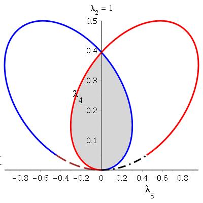
70 Figure 3.8: Different angles of Λ µ Figure 3.9: Different slices through λ 2 55

71 Figure 3.10: Different slices through λ 4 Geometry of Λ µ of LMM of a normal distribution with unknown σ is also of interest, as the boundary planes clearly depend on the value of σ. Figure 3.11 illustrates that changing value of σ does not alter the geometry of the Λ µ, but just acts as a scaler and inflate the subspace. Figure 3.11: The hard boundary for σ = 1 (blue) vs σ = 1.2 (red) Conjecture 3.1 Suppose Λ σ µ is the parameter subspace of the LMM of the normal model N(µ, σ 2 ). If σ 1 < σ 2, then Λ σ 1 µ Λ σ 2 µ. 56

72 Since normal distribution with unknown σ has two parameters, its LMM is an overparametrized model, which causes an identifiability problem. To see explicitly, consider a LMM of a normal model with σ = 1 and an unmixed normal distribution with unknown σ. For the LMM of N(µ, 1) we have E [ (X µ) 2] = 1 + 2λ 2 E [ (X µ) 3] = 6λ 3 E [ (X µ) 4] = 12λ λ (3.5.8) the same central moments for the unmixed model N(µ, σ 2 ), unknown σ, are E [ (X µ) 2] = σ 2, E [ (X µ) 3] = 0, E [ (X µ) 4] = 3σ 4 (3.5.9) equating these two sets of central moments we get a curve as a function of σ 2 inside Λ µ [ ] λ 2 (σ 2 ) = σ2 1, λ 3 (σ 2 ) = 0, λ 4 (σ 2 ) = 3σ 4 6σ That is up to forth moments we can represent the N(µ, σ 2 ) by the LMM of N(µ, 1) with characterized values of λ j s. Exponential Model Similar to the LMM of a normal distribution, the boundary of Λ µ for an exponential distribution is obtained by intersection of infinite number of half-spaces and can be constructed by their envelope. Illustrated in Figure 3.12, the boundary of Λ µ is a locally smooth selfintersecting surface with singularity curves. The 2-dimensional slices of Λ µ in Figure 3.13 illustrates the position of the singularities as points of the singularity curves. Inspection shows that these points also correspond to quartics with two double roots, as in the normal models Surface Parametrization and Optimization Section and characterize the hard and soft boundaries of the LMM of a normal distribution as ruled surfaces. Specifically, any point λ = (λ 2, λ 3, λ 4 ) restricted to these 57

73 Figure 3.12: Different angles of Λ µ for f(x, µ) = µ e µx Figure 3.13: Different slices through λ 4, for f(x, µ) = µ e µx surfaces is uniquely determined by a pair (x, u). In this section, we exploit this parameterization for finding the maximum likelihood estimate of λ on these boundaries. Let D be the envelope of the family of planes in Equation (3.3.5). For a fixed µ, the loglikelihood 58

74 function restricted to D is a function of (x, u) as follows l D (x, u) = n { log f(x; µ) + 4 } λ j(x, u) f (j) (x i ; µ). (3.5.10) i=1 j=2 However, a searching algorithm using the basis of coordinates (x, u) may not retain efficient steps, since they are not orthogonal. Hence, we need to find an alternative parameterization such that the corresponding basis are orthogonal. That is, instead of (x, u) parametrization, any point on the D is characterized by (x 1, x 0 ) implying orthogonal directions. Orthogonal Parametrization For finding an orthogonal parameterization on a ruled surface, we directly use the geometry of smooth space curves and their related geometric concepts such as, normal vectors, binormal vectors, tangent planes and normal planes (Struik, 1988, ch.1). At any regular point λ(x 1 ) on C(x) the normal plane π x1 is orthogonal to C(x), and t(x 1 ) is the normal vector to π x1. Also π x1 is spanned by the normal vector n(x 1 ) and binormal vectors b(x 1 ) of C(x). In addition, for the normalized vectors t(x 1 ), n(x 1 ) and b(x 1 ), we have the following equations, t(x 1 ) b(x 1 ) = 0, n(x 1 ) b(x 1 ) = 0, b(x 1 ) b(x 1 ) = 1, (3.5.11) where represents the regular inner product in Euclidean space. t(x 1 ) and n(x 1 ) are obtained from the first and second derivatives of C(x) at x 1, and, b(x 1 ) can be calculated from the equations in (3.5.11). To obtain an orthogonal parametrization on D, we characterize each point on D using the normal plane π x1 to C at a suitable point, say λ(x 1 ). In other words, for a λ D, represented by (x 0, u 0 ), we want to find (x 1, v, w), where v and w are fully determined by x 0 and x 1 (see Figure 3.14). For any λ D, there is a normal plane π x1 which intersects C(x) at λ(x 1 ) and includes λ, and can be represented by both implicit and explicit equations as follows, π x1 = π x1 = { } λ R 3 λ = λ(x1 ) + v n(x 1 ) + w b(x 1 ), v, w R { } λ R 3 (λ λ(x1 )) t(x 1 ) = 0. (3.5.12) 59

75 λ(x) πx 1 n(x 1 ) λ(x 1 ) λ(x 0 ) b(x 1 ) λx 0 Lx 0 Cx1 λx 1 λ(x 1 ) Figure 3.14: A schematic graph for visualizing the orthogonal reparametrization The intersection of π x1 and D is a plane curve on π x1, say C x1, such that it can be also spanned by the orthonormal bases n(x 1 ) and b(x 1 ), considering λ(x 1 ) as the origin of π x1. On the other hand, according to ruled surface parameterization, λ is represented by a pair (x 0, u 0 ) as follows λ = λ(x 0 ) + u 0 t(x 0 ), (3.5.13) which is a point on the line L x0 = λ(x 0 ) + u t(x 0 ). (3.5.14) Therefore, λ can be determined as the intersecting point of π x1 and L x0 ; that is, we need to find u 0 such that λ satisfies equation (3.5.13). For a fixed x 1, if the equation in (3.5.13) is substituted in the second equation in (3.5.12), after some algebra, u 0 is obtained as a function of x 0 as follows, Hence, λ can be written as u(x 0 ) = (λ(x 1) λ(x 0 )) t(x 1 ). (3.5.15) t(x 0 ) t(x 1 ) λ x0 = λ(x 0 ) + u(x 0 ) t(x 0 ), (3.5.16) which is also spanned by n(x 1 ) and b(x 1 ), thus we can write λ x0 = λ(x 1 ) + v x1 (x 0 ) n(x 1 ) + w x1 (x 0 ) b(x 1 ), (3.5.17) 60

76 where v x1 (x 0 ) = (λ x0 λ(x 1 )) n(x 1 ), w x1 (x 0 ) = (λ x0 λ(x 1 )) b(x 1 ). Therefore, for any λ D there is a unique pair (x 1, x 0 ) where λ(x 1, x 0 ) = λ(x 1 ) + v x1 (x 0 ) n(x 1 ) + w x1 (x 0 ) b(x 1 ), x 0, x 1 R (3.5.18) According to this new orthogonal parametrization the loglikelihood function in Equation (3.5.10) can be written as follows, l D (x 1, x 0 ) = n { log f(x; µ) + 4 } λ j(x 1, x 0 ) f (j) (x i ; µ) i=1 j=2 (3.5.19) Figure 3.15 shows D with the new parameterization and the contours of l D (x 1, x 0 ) for a sample of size n = 20. The surface is in three pieces as the result of the singularity points in the edge of regression. However, each piece is quite well behaved on which any gradient based searching algorithm can be employed for finding the maximum point. Figure 3.15: Contour plat of the loglikelihood function on the boundary surface D. Left: for 1 < x 0 < 1 where x 0 = 0, represents the cusp in the edge of regression. Middle: for x 0 > 1. Right: the whole surface where it splits as the result of the two asymptotes at x 0 = ±